Convergence rates of adaptive methods - CiteSeerX

arXiv:1408.3889v1 [math.NA] 18 Aug 2014

Convergence rates of adaptive methods, Besov spaces, and multilevel approximation Tsogtgerel Gantumur McGill University Abstract This paper concerns characterizations of approximation classes associated to adaptive finite element methods with isotropic h-refinements. It is known from the seminal work of Binev, Dahmen, DeVore and Petrushev that such classes are related to Besov spaces. The range of parameters for which the inverse embedding results hold is rather limited, and recently, Gaspoz and Morin have shown, among other things, that this limitation disappears if we replace Besov spaces by suitable approximation spaces associated to finite element approximation from uniformly refined triangulations. We call the latter spaces multievel approximation spaces, and argue that these spaces are placed naturally halfway between adaptive approximation classes and Besov spaces, in the sense that it is more natural to relate multilevel approximation spaces with either Besov spaces or adaptive approximation classes, than to go directly from adaptive approximation classes to Besov spaces. In particular, we prove embeddings of multilevel approximation spaces into adaptive approximation classes, complementing the inverse embedding theorems of Gaspoz and Morin. Furthermore, in the present paper, we initiate a theoretical study of adaptive approximation classes that are defined using a modified notion of error, the so-called total error, which is the energy error plus an oscillation term. Such approximation classes have recently been shown to arise naturally in the analysis of adaptive algorithms. We first develop a sufficiently general approximation theory framework to handle such modifications, and then apply the abstract theory to second order elliptic problems discretized by Lagrange finite elements, resulting in characterizations of modified approximation classes in terms of memberships of the problem solution and data into certain approximation spaces, which are in turn related to Besov spaces. Finally, it should be noted that throughout the paper we paid equal attention to both the newest vertex bisection and the red refinement procedures.

Contents 1 2 2.1 2.2 2.3

Introduction . . . . . . . . . . . . . . . . . . . . . . . . General theorems . . . . . . . . . . . . . . . . . . . . . The setup . . . . . . . . . . . . . . . . . . . . . . . . . Direct embeddings for standard approximation classes Direct embeddings for general approximation classes . 1

. . . . .

. . . . .

. . . . .

. . . . .

. . . . .

. . . . .

. . . . .

. . . . .

. . . . .

. . . . .

. . . . .

. . . . .

2 6 6 9 12

1 Introduction

2.4 3 3.1 3.2 3.3 3.4 3.5 4 4.1 4.2 A

1

2

Inverse embeddings . . . . . . . . . . . . . . . . . . . Lagrange finite elements . . . . . . . . . . . . . . . . Besov spaces on bounded domains . . . . . . . . . . Quasi-interpolation operators . . . . . . . . . . . . . Multilevel approximation spaces . . . . . . . . . . . Adaptive approximation . . . . . . . . . . . . . . . . Discontinuous piecewise polynomials . . . . . . . . . Second order elliptic problems . . . . . . . . . . . . . Introduction . . . . . . . . . . . . . . . . . . . . . . . A characterization of adaptive approximation classes Tree completion and the red refinement . . . . . . .

. . . . . . . . . . .

. . . . . . . . . . .

. . . . . . . . . . .

. . . . . . . . . . .

. . . . . . . . . . .

. . . . . . . . . . .

. . . . . . . . . . .

. . . . . . . . . . .

. . . . . . . . . . .

. . . . . . . . . . .

. . . . . . . . . . .

. . . . . . . . . . .

. . . . . . . . . . .

14 17 17 18 24 29 33 37 37 39 42

Introduction

Among the most important achievements in theoretical numerical analysis during the last decade was the development of mathematical techniques for analyzing the performance of adaptive finite element methods. A crucial notion in this theory is that of approximation classes, which we discuss here in a simple but very paradigmatic setting. Given a polygonal domain Ω ∈ R2 , a conforming triangulation P0 of Ω, and a number s > 0, we say that a function u on Ω belongs to the approximation class A s if for each N , there is a conforming triangulation P of Ω with at most N triangles, such that P is obtained by a sequence of newest vertex bisections from P0 , and that u can be approximated by a continuous piecewise affine function subordinate to P with the error bounded by cN −s , where c = c(u, P0 , s) ≥ 0 is a constant independent of N . In a typical setting, the error is measured in the H 1 -norm, which is the natural energy norm for second order elliptic problems. To reiterate and to remove any ambiguities, we say that u ∈ H 1 (Ω) belongs to A s if min

inf ku − vkH 1 ≤ cN −s ,

{P ∈P:#P ≤N } v∈SP

(1)

for all N ≥ #P0 and for some constant c, where P is the set of conforming triangulations of Ω that are obtained by a sequence of newest vertex bisections from P0 , and SP is the space of continuous piecewise affine functions subordinate to the triangulation P . Approximation classes can be used to reveal a theoretical barrier on any procedure that is designed to approximate u by means of piecewise polynomials and a fixed refinement rule such as the newest vertex bisection. Suppose that we start with the initial triangulation P0 , and generate a sequence of conforming triangulations by using newest vertex bisections. Suppose also that we are trying to capture the function u by using continuous piecewise linear functions subordinate to the generated triangulations. Finally, assume that u ∈ A s but u 6∈ A σ for any σ > s. Then as far as the exponent σ in cN −σ is concerned, it is obvious that the best asymptotic bound on the error we can hope for is cN −s , where N is the number of triangles. Now supposing that u is given as the solution of a boundary value

1 Introduction

3

problem, a natural question is if this convergence rate can be achieved by any practical algorithm, and it was answered in the seminal works of Binev, Dahmen, and DeVore (2004) and Stevenson (2007): These papers established that the convergence rates of certain adaptive finite element methods are optimal, in the sense that if u ∈ A s for some s > 0, then the method converges with the rate not slower than s. One must mention the earlier developments D¨ orfler (1996); Morin, Nochetto, and Siebert (2000); Cohen, Dahmen, and DeVore (2001); Gantumur, Harbrecht, and Stevenson (2007), which paved the way for the final achievement. Having established that the smallest approximation class A s in which the solution u belongs to essentially determines how fast adaptive finite element methods converge, the next issue is to determine how large these classes are and if the solution to a typical boundary value problem would belong to an A s with large s. In particular, one wants to compare the performance of adaptive methods with that of non-adaptive ones. A first step towards addressing this issue is to characterize the approximation classes in terms of classical smoothness spaces, and the main work in this direction so far appeared is Binev, Dahmen, DeVore, and Petrushev (2002), which, upon tailoring to our situation and a slight α ⊂ A s ⊂ B σ for 2 = σ < 1 + 1 and σ < α < max{2, 1 + 1 } simplification, tells that Bp,p p,p p p p α are the standard Besov spaces defined on Ω. This result has with s = α−1 . Here B p,q 2 recently been generalized to higher order Lagrange finite elements by Gaspoz and Morin α ⊂ A s holds in the larger (2013). In particular, they show that the direct embedding Bp,p range σ < α < m+max{1, p1 }, where m is the polynomial degree of the finite element space, σ see Figure 1(a). However, the restriction σ < 1 + p1 on the inverse embedding A s ⊂ Bp,p cannot be removed, since for instance, any finite element function whose derivative is σ if σ ≥ 1+ 1 and p < ∞. To get around this problem, Gaspoz discontinuous cannot be in Bp,p p σ by the approximation space Aσ and Morin proposed to replace the Besov space Bp,p p,p 1 associated to uniform refinements . We call the spaces Aσp,p multilevel approximation spaces, and their definition will be given in Subsection 3.3. For the purposes of this introduction, and roughly speaking, the space Aσp,p is the collection of functions u ∈ Lp for which inf ku − vkLp ≤ chσk ,

v∈SPk

(2)

where {Pk } ⊂ P is a sequence of triangulations such that Pk+1 is the uniform refinement of Pk , and hk is the diameter of a typical triangle in Pk . Note for instance that finite element functions are in every Aσp,p . With the multilevel approximation spaces at hand, the inverse embedding A s ⊂ Aσp,p is recovered for all σ = p2 . In this paper, we prove the direct embedding Aαp,p ⊂ A s , so that the existing situation α ⊂ A s ⊂ Aσ is improved to Aα ⊂ A s ⊂ Aσ . It is a genuine improvement, since Bp,p p,p p,p p,p α α (Ω) for α ≥ 1 + 1 . Moreover, as one stays entirely within an approximation Ap,p (Ω) ) Bp,p p σ ˆp,p This space is denoted by B in Gaspoz and Morin (2013). In the present paper we are adopting the notation of Oswald (1994). 1

1 Introduction

4

theory framework, one can argue that the link between A s and Aαp,p is more natural than α . Once the link between A s and Aα has been established, the link between A s and Bp,p p,p α . It seems that this one can then invoke the well known relationships between Aαp,p and Bp,p two step process offers more insight into the underlying phenomenon. We also remark that while the existing results are only for the newest vertex bisection, we take into account the red refinement procedure as well. α

α

α Bp,p m+1

α Bp,p

1 2

2 1

1

H

L2

1

1 p

H −1 1 2

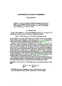
α (b) If the space Bp,p is located above or on the solid line, and if u ∈ A s and α s with s = α+1 ∆u ∈ Bp,p 2 , then u ∈ A∗ . It is as if the approximation of ∆u is taking place in H −1 , with the proviso that the shaded area is excluded from all considerations.

1 p

α is located strictly above (a) If the space Bp,p the solid line and below the dashed line, α then Bp,p ⊂ A s with s = α−1 2 . The α hold inverse embeddings A s+ε ⊂ Bp,p on the solid line and below the (slanted) dotted line.

α . Fig. 1: Illustration of various embeddings. The point ( p1 , α) represents the space Bp,p

The approximation classes A s defined by (1) are associated to measuring the error of an approximation in the H 1 -norm. Of course, this can be generalized to other function α , which we will consider in Section 3. However, we will space norms, such as Lp and Bp,p not stop there, and consider more general approximation classes corresponding to ways of measuring the error between a general function u and a discrete function v ∈ SP by a quantity ρ(u, v, P ) that may depend on the triangulation P and is required to make sense merely for discrete functions v ∈ SP . An example of such an error measure is !1 2 X (diam τ )2 kf − Πτ f k2L (τ ) ρ(u, v, P ) = ku − vk2H 1 + , (3) 2

τ ∈P

where f = ∆u, and Πτ : L2 (τ ) → Pd is the L2 (τ )-orthogonal projection onto Pd , the space of polynomials of degree not exceeding d. It has been shown in Cascon, Kreuzer, Nochetto,

1 Introduction

5

and Siebert (2008) that if the solution u of the boundary value problem ∆u = f

in Ω

and

u|Ω = 0,

(4)

inf ρ(u, v, P ) ≤ cN −s ,

(5)

satisfies min

{P ∈P:#P ≤N } v∈SP

for all N ≥ #P0 and for some constants c and s > 0, then a typical adaptive finite element method for solving (4) converges with the rate not slower than s. Moreover, there are good reasons to consider that the approximation classes A∗s defined by the condition (5) are more attuned to certain practical adaptive finite element methods than the standard approximation classes A s defined by (1), see Section 4. Obviously, we have A∗s ⊂ A s but we cannot expect the inclusion A s ⊂ A∗s to hold in general. In Cascon et al. (2008), an effective characterization of A∗s was announced as an important pending issue. In the present paper, we establish a characterization of A∗s in terms of memberships of u and f = ∆u into suitable approximation spaces, which in turn are related to Besov α with α ≥ 1 − 1 and s = α+1 , spaces. For instance, we show that if u ∈ A s and f ∈ Bp,p 2 p 2 2 then u ∈ A∗s , see Figure 1(b). Note that the approximation rate s = α+1 2 is as if we were approximating f in the H −1 -norm, which is illustrated by the arrow downwards. However, the parameters must satisfy α2 ≥ p1 − 12 (above or on the solid line), which is more restrictive 1 1 compared to α+1 2 > p − 2 (above the dashed line), the latter being the condition we would expect if the approximation was indeed taking place in H −1 . This situation cannot be α 6⊂ L , hence the quantity (3) would improved in the sense that if α2 < p1 − 12 then Bp,p 2 α be infinite in general for f ∈ Bp,p . In Section 4, we treat a more general class of variable coefficient second order equations. As a rule, the actual results therein are in terms of the approximation spaces that are studied in Section 3, which means that Besov spaces are rarely mentioned, and one has to appeal to Section 3 in order to deduce statements such as the one we have just described. The results of Section 4 and some of the results of Section 3 are proved by invoking abstract theorems that are established in Section 2. These theorems extend some of the standard results from approximation theory to deal with generalized approximation classes such as A∗s . We decided to consider a fairly general setting in the hope that the theorems will be used for establishing characterizations of other approximation classes. For example, adaptive boundary element methods and adaptive approximation in finite element exterior calculus seem to be amenable to our abstract framework, although checking the details poses some technical challenges. This paper is organized as follows. In Section 2, we introduce an abstract framework that is more general than usually considered in approximation theory of finite element methods, and collect some theorems that can be used to prove embedding theorems between adaptive approximation classes and other function spaces. In Section 3, we recall some standard results on multilevel approximation spaces and their relationships with Besov

2 General theorems

6

spaces, and then prove direct embedding theorems between multilevel approximation spaces and adaptive approximation classes. The main results of this section are Theorem 3.7, Theorem 3.8, Theorem 3.11, and Theorem 3.12. In Section 4, we investigate approximation classes associated to certain adaptive finite element methods for second order boundary value problems. Finally, in the appendix, we establish some technical estimates on the complexity of completions of triangulations obtained by the red refinement rule.

2 2.1

General theorems The setup

Let M be an n-dimensional topological manifold, equipped with a compatible measure, in the sense that all Borel sets are measurable. What we have in mind here is M = Rn with the Lebesgue measure on it, or a piecewise smooth surface M ⊂ RN with its canonical Hausdorff measure. With Ω ⊂ M a bounded domain, we consider a class of partitions (triangulations) of Ω, and finite element type functions defined over those partitions. Ultimately, we are interested in characterizing those functions on Ω that can be well approximated by such finite element type functions. In order to make these concepts precise, we will use in this section a fairly abstract setting, which we believe to be a good compromise between generality and readability. By a partition of Ω Swe understand a collection P of finitely many disjoint open subsets of Ω, satisfying Ω = τ ∈P τ . We assume that a set P of partitions of Ω is given, which we call the set of admissible partitions. For simplicity, we will assume that for any k ∈ N the set {P ∈ P : #P ≤ k} is finite. In practice, P would be, for instance, the set of all conforming triangulations obtained from a fixed initial triangulation P0 by repeated applications of the newest vertex bisection procedure. Another important example arises from the red refinement rule. In this case, the admissibility criterion on a partition would be either that the number of hanging nodes per edge is bounded by a prescribed finite number, or that the diameter ratio between neighbouring elements stays bounded by a prescribed constant. Here and in the following, we often write triangles and edges et cetera to mean n-simplices and (n − 1)-dimensional faces et cetera, which seems to improve readability. We will assume the existence of a refinement procedure satisfying certain requirements. Given a partition P ∈ P and a set R ⊂ P of its elements, the refinement procedure produces P 0 ∈ P, such that P \ P 0 ⊃ R, i.e., the elements in R are refined at least once. Let us denote it by P 0 = refine(P, R). In practice, this is implemented by a usual naive refinement possibly producing a non-admissible partition, followed by a so-called completion procedure. We assume the existence of a constant λ > 1 such that |τ | ≤ λ−n |σ| for all τ ∈√P 0 and σ ∈ R with τ ∩ σ 6= ∅. Note that we have λ = 2 for red refinements, and λ = n 2 for the newest vertex bisection. Moreover, we assume the following on the efficiency of the refinement procedure: If {Pk } ⊂ P and {Rk } are sequences such that

2 General theorems

7

Pk+1 = refine(Pk , Rk ) and Rk ⊂ Pk for k = 0, 1, . . ., then #Pk − #P0 .

k−1 X

#Rm ,

k = 1, 2, . . . .

(6)

m=0

This assumption is justified for newest vertex bisection algorithm in Binev et al. (2004); Stevenson (2008), and demonstrated for a 1D refinement rule in Aurada, Feischl, F¨ uhrer, Karkulik, and Praetorius (2012). The general red refinement procedure is treated in the appendix of this paper. Next, we shall introduce an abstraction of finite element spaces. To this end, we assume that there is a quasi-Banach space X0 , and for each P ∈ P, there is a nontrivial, finite dimensional subspace SP ⊂ X0 . The space X0 models the function space over Ω in which the approximation takes place, such as X0 = H t (Ω) and X0 = Lp (Ω). The spaces SP are, as the reader might have guessed, models of finite element spaces, from which we approximate general functions in X0 . Obviously, a natural notion of error between an element u ∈ X0 and its approximation v ∈ SP is the quasi-norm ku − vkX0 . However, we need a bit more flexibility in how to measure such errors, and so we suppose that there is a function ρ(u, v, P ) ∈ [0, ∞] defined for u ∈ X0 , v ∈ SP , and P ∈ P. Note that this error measure, which we call a distance function, can depend on the partition P , and it is only required to make sense for functions v ∈ SP . We allow the value ρ = ∞ to leave open the possibility that for some u ∈ X0 we have ρ(u, ·, ·) = ∞. The most important distance function is still ρ(u, v, P ) = ku − vkX0 , but other examples will appear later in the paper, see e.g., Example 2.7, Subsection 3.5 and Section 4. Given u ∈ X0 and P ∈ P, we let E(u, SP )ρ = inf ρ(u, v, P ),

(7)

v∈SP

which is the error of a best approximation of u from SP . Furthermore, we introduce Ek (u)ρ =

inf

{P ∈P:#P ≤2k N }

E(u, SP )ρ ,

(8)

for u ∈ X0 and k ∈ N, with the constant N chosen sufficiently large in order to ensure that the set {P ∈ P : #P ≤ 2N } is nonempty. In a certain sense, Ek (u)ρ is the best approximation error when one tries to approximate u within the budget of 2k N triangles. Finally, we define the main object of our study, the (adaptive) approximation class Aqs (ρ) = Aqs (ρ, P, {SP }) = {u ∈ X0 : |u|Aqs (ρ) < ∞},

(9)

where s > 0 and 0 < q ≤ ∞ are parameters, and |u|Aqs (ρ) = k(2ks Ek (u)ρ )k∈N k`q ,

u ∈ X0 .

(10)

2 General theorems

8

s (ρ). Note that u ∈ A s (ρ) In the following, we will use the abbreviation A s (ρ) = A∞ q implies Ek (u)ρ ≤ c2−ks for all k and for some constant c, and these two conditions are equivalent if q = ∞. We have Aqs (ρ) ⊂ Ars (ρ) for q ≤ r, and Aqs (ρ) ⊂ Arα (ρ) for s > α and for any 0 < q, r ≤ ∞. The set Aqs (ρ) is not a linear space without further assumptions on ρ and P. However, in a typical situation, it is indeed a vector space equipped with the quasi-norm k · kAqs (ρ) = k · kX0 + | · |Aqs (ρ) .

Remark 2.1. Suppose that ρ satisfies

• ρ(αu, αv, P ) = |α|ρ(u, v, P ) for α ∈ R, and • ρ(u + u0 , v + v 0 , P ) . ρ(u, v, P ) + ρ(u0 , v 0 , P ). Then |·|Aqs (ρ) is a quasi-seminorm, in the sense that it is positive homogeneous and satisfies the generalized triangle inequality. Moreover, Aqs (ρ) is a quasi-normed vector space. If only the second condition holds, then Aqs (ρ) would be a quasi-normed abelian group, in the sense of Bergh and L¨ ofstr¨ om (1976). Even though we will not use this fact, it is worth noting that ρ has the aforementioned properties for all applications we have in mind. We call the approximation classes associated to ρ(u, v, ·) = ku − vkX0 standard approximation classes, and write Aqs (X0 ) ≡ Aqs (ρ) and A s (X0 ) ≡ A s (ρ). We want to characterize A s (ρ) in terms of an auxiliary quasi-Banach space X ,→ X0 . α , with α > 1 − 1 . We assume The main examples to keep in mind are X0 = Lp and X = Bq,q n q p that the space X has the following local structure: There exist a constant 0 < q < ∞, and a function | · |X(G) : X → R+ associated to each open set G ⊂ Ω, such that X k

|u|qX(τk ) . kukqX

(u ∈ X),

(11)

for any finite sequence {τk } ⊂ P of non-overlapping elements taken from any P ∈ P. Finally, for any τ ∈ P with P ∈ P, we let τˆ ⊂ Ω be a domain containing τ , which will, in a typical situation, be the union of elements of P surrounding τ . We express the dependence of τˆ on P as τˆ = P (τ ). Then as an extension of the above sub-additivity property, we assume that X q |u|X(Pk (τk )) . kukqX (u ∈ X), (12) k

for any finite sequences {Pk } ⊂ P and {τk }, with τk ∈ Pk and {τk } non-overlapping. A trivial example of such a structure is X = Lq (Ω) with | · |X(G) = k · kLq (G) . Here the subadditivity (12) can be guaranteed if the underlying triangulations satisfy a certain local finiteness property.

2 General theorems

2.2

9

Direct embeddings for standard approximation classes

The following theorem shows that the inclusion X ⊂ A s (ρ) can be proved by exhibiting a direct estimate. A direct application of this criterion is mainly useful for deriving embeddings of the form X ⊂ A s (X0 ). In the next subsection, it will be generalized to a criterion that is valid in a more complex situations. Theorem 2.2. Let 0 0. Then for any k ∈ N sufficiently large there exists a partition P ∈ P with #P ≤ k satisfying !1

p

X τ ∈P

pδ

|τ |

|u|pX(ˆτ )

. k −s kukX ,

(13)

with s = δ+ 1q − p1 > 0, where τˆ = P (τ ) is as in (12), and the case p = ∞ must be interpreted in the usual way (with a maximum replacing the discrete p-norm). In particular, if u ∈ X satisfies !1 p X |τ |pδ |u|pX(ˆτ ) , (14) E(u, SP )ρ . for all P ∈ P, then we have u ∈ A

s (ρ)

τ ∈P

with |u|A s (ρ) . kukX .

Proof. What follows is a slight abstraction of the proof of Proposition 5.2 in Binev et al. (2002); we include it here for completeness. We first deal with the case 0 0, and any P0 ∈ P, below we will specify a procedure to generate a partition P ∈ P satisfying X e(τ, P ) ≤ c0 (#P )ε, (16) τ ∈P

and

p/(1+ps)

#P − #P0 ≤ cε−1/(1+ps) kukX

,

(17)

where c0 depends only on the implicit constant of (14), and c depends only on |Ω|, λ, and the implicit constants of (6), and (12). Then, for any given k > 0, by choosing ε = (c/k)1+ps kukpX , we would be able to guarantee a partition P ∈ P satisfying #P ≤ #P0 + k and X e(τ, P ) . k −sp kukpX . τ ∈P

(18)

(19)

2 General theorems

10

This would imply the lemma, as k −s can be replaced by (#P0 + k)−s for, e.g., k ≥ #P0 . Let ε > 0 and let P0 ∈ P. We then recursively define Rk = {τ ∈ Pk : e(τ, Pk ) > ε} and Pk+1 = refine(Pk , Rk ) for k = 0, 1, . . .. For all sufficiently large k we will have Rk = ∅ since |u|X(ˆτ ) . kukX by (12), and |τ | is reduced by a constant factor µ = λ−n < 1 at each refinement. Let P = Pk , where k marks the first occurrence of Rk = ∅. Then combining (14) with (15), and taking into account that e(τ, Pk ) ≤ ε for τ ∈ Pk , we obtain (16). In order to get a bound on #P , we estimate the cardinality of R = R0 ∪ R1 ∪ . . . ∪ Rk−1 , and use (6). Let Λj = {τ ∈ R : µj+1 ≤ |τ | < µj } for j ∈ Z, and let mj = #Λj . Note that the elements of Λj (for any fixed j) are disjoint, since if any two elements intersect, then they must come from different Rk ’s as each Rk consists of disjoint elements, and hence by assumption on the refinement procedure, the ratio between the measures of the two elements must lie outside (µ, µ−1 ). This gives the trivial bound mj ≤ µ−j−1 |Ω|.

(20)

On the other hand, we have e(τ, Pk ) > ε for τ ∈ Λj with some k, which gives ε < |τ |pδ |u|pX(ˆτ ) < µjpδ |u|pX(ˆτ ) ,

(21)

where τˆ is defined with respect to Pk , and k may depend on τ . Summing over τ ∈ Λj , we get X q (22) |u|X(ˆτ ) . µjqδ kukqX , mj εq/p ≤ µjqδ τ ∈Λj

where we have used (12). Finally, summing for j, we obtain #R ≤

∞ X j=−∞

mj .

∞ X j=−∞

o n q/(1+qδ) , min µ−j , ε−q/p µjqδ kukqX . ε−q/(p+pqδ) kukX

(23)

which, in view of (6) and q/(1 + qδ) = p/(1 + ps), establishes the bound (17). We only sketch the case p = ∞ since the proof is essentially the same. We use e(τ, P ) = |τ |δ |u|X(ˆτ ) ,

(24)

instead of (15), and run the same algorithm. This guarantees that the resulting partition P satisfies max e(τ, P ) ≤ ε. (25) τ ∈P

We bound the cardinality of P in the same way, which formally amounts to putting p = 1 into (21) and proceeding. The final result is q/(1+qδ)

#P − #P0 ≤ cε−q/(1+qδ) kukX where s = δ + 1q . The proof is complete.

1/s

= cε−1/s kukX ,

(26)

2 General theorems

11

Example 2.3. The main argument of the preceding proof can be traced back to Birman and Solomyak (1967). Recently, in Binev et al. (2002), this argument was applied to obtain an embedding of a Besov space into A s (X0 ), i.e., the case where the distance function ρ is given by ρ(u, v, ·) = ku − vkX0 . We want to include here one such application. Let Ω ⊂ Rn be a bounded polyhedral domain with Lipschitz boundary, and take P to be the set of conforming triangulations of Ω obtained from a fixed conforming triangulation P0 by means of newest vertex bisections. For P ∈ P, let SP be the Lagrange finite element space of continuous piecewise polynomials of degree not exceeding m. Thus, for instance, the piecewise linear finite elements would correspond to m = 1. Moreover, for P ∈ P S and τ ∈ P , let τˆ = P (τ ) be the interior of {σ : σ ∈ P, σ ∩ τ 6= ∅}. Finally, let us put α (Ω), and ρ(u, v, ·) = ku − vk X0 = Lp (Ω), X = Bq,q Lp (Ω) . Then in this setting, the estimate α 1 (14) holds with the parameters p and δ = n + p − 1q , as long as 0 < α < m + max{1, 1q } and δ > 0, cf. Binev et al. (2002); Gaspoz and Morin (2013). Hence the preceding lemma α (Ω) ,→ A s (L (Ω)) with s = α . immediately implies that Bq,q p n In the rest of this subsection, we want to record some results involving interpolation spaces. For u ∈ X0 and t > 0, the K-functional is K(u, t; X0 , X) = inf (ku − vkX0 + tkvkX ) , v∈X

(27)

and for 0 < θ < 1 and 0 < γ ≤ ∞, we define the (real) interpolation space (X0 , X)θ,γ as the space of functions u ∈ X0 for which the quantity

|u|(X0 ,X)θ,γ = [λθm K(u, λ−m ; X0 , X)]m≥0 , (28) `γ

is finite. These are quasi-Banach spaces with the quasi-norms k · kX0 + | · |(X0 ,X)θ,γ . The parameter λ > 1 can be chosen at one’s convenience, because the resulting quasi-norms are all pairwise equivalent. Corollary 2.4. Let 0 0 and let s = δ +

1 q

− p1 > 0. Let !1 p

E(u, SP )X0 .

X τ ∈P

|τ |

pδ

|u|pX(ˆτ )

,

(29)

for all u ∈ X and P ∈ P. Then we have (X0 , X)α/s,γ ⊂ Aγα (X0 ) for 0 < α < s and 0 < γ ≤ ∞. Proof. For u, v ∈ (X0 , X)α/s,γ , we have

Ek (u)X0 . ku − vkX0 + Ek (v)X0 ,

(30)

By Theorem 2.2, for v ∈ X we have Ek (v)X0 . 2−ks kvkX , leading to Ek (u)X0 . ku − vkX0 + 2−ks kvkX .

After minimizing over v ∈ X, the right hand side gives the K-functional and (28) implies that u ∈ Aγα (X0 ).

(31) K(u, 2−ks ; X0 , X),

2 General theorems

2.3

12

Direct embeddings for general approximation classes

As mentioned in the introduction, our study is motivated by algorithms for approximating the solution of the operator equation T u = f . Hence it should not come as a surprise that we assume the existence of a continuous operator T : X0 → Y0 , with Y0 a quasi-Banach space. An example to keep in mind is the Laplace operator sending H01 onto H −1 . In this subsection we do not assume linearity, although all examples of T we have in this paper are linear. We also need an auxiliary quasi-Banach space Y ,→ Y0 , satisfying the properties analogous to that of X, in particular, (12) with some 0 < r < ∞ replacing q there. If σ−1 with σ > 1 − 1 . Y0 = H −1 , a typical example of Y would be Br,r n r 2 s s It is obvious that A (ρ) ⊂ A (X0 ), provided we have ku − vkX0 . ρ(u, v, ·). The latter condition is satisfied for all practical applications we have in mind. We will shortly present a theorem providing a criterion for answering questions such as A s (X0 )∩T −1 (Y ) ⊂ A s (ρ). Before stating the theorem, we need to introduce a bit more structure on the set P. The structure we need is that of overlay of partitions: We assume that there is an operation ⊕ : P × P → P satisfying SP + SQ ⊂ SP ⊕Q ,

#(P ⊕ Q) . #P + #Q,

and

(32)

for P, Q ∈ P. In addition, we will assume that ρ(u, v, P ⊕ Q) . ρ(u, v, P ).

(33)

In the conforming world, P ⊕ Q can be taken to be the smallest and common conforming refinement of P and Q, for which (32) is demonstrated in Stevenson (2007), see also Cascon et al. (2008). The same argument works for the red refinement rule, cf. Aurada et al. (2012). Theorem 2.5. Let 0 0, and let s = δ + u ∈ A s (X0 ) ∩ T −1 (Y ) satisfies

1 r

−

1 p

> 0. Assume that

!1

p

E(u, SP )ρ . E(u, SP )X0 +

X τ ∈P

pδ

|τ |

|T u|pY (ˆτ )

,

(34)

for all P ∈ P (in particular E(u, ·)ρ is always finite). Suppose also that 1



!1

p

X  τ ∈P ⊕Q

pδ

|τ |

|T u|pY (ˆτ ) 

p

.

X τ ∈P

pδ

|τ |

|T u|pY (ˆτ )

,

(35)

for any P, Q ∈ P. Then we have u ∈ A s (ρ) with |u|A s (ρ) . |u|A s (X0 ) + kT ukY .

Proof. Let k ∈ N be an arbitrary number. Then by definition of A s (X0 ), there exists a partition P 0 ∈ P such that E(u, SP 0 )X0 ≤ 2−ks |u|A s (X0 ) ,

and

#P 0 ≤ 2k N.

(36)

2 General theorems

13

Similarly, by applying Theorem 2.2 with the roles of X and Y , and those of u and T u reversed, respectively, we can generate a partition P 00 ∈ P such that !1

p

X τ ∈P 00

|τ |pδ |T u|pY (ˆτ )

. 2−ks kT ukY ,

#P 00 ≤ 2k N.

and

(37)

Then for P = P 0 ⊕ P 00 we have #P . 2k by (32). Moreover, (35) together with the obvious monotonicity E(u, SP )X0 ≤ E(u, SP 0 )X0 , (38)

guarantee that the right hand side of (34) is bounded by a multiple of 2−ks (|u|A s (X0 ) + kT ukY ), which completes the proof.

Remark 2.6. By the same argument, one can establish more general results, say, with an additional term involving E(u, SP )ρ1 in the right hand side of (34), where ρ1 is some distance function. We do not state such generalizations, but will use them on occasions later in the paper, cf. the proof of Theorem 4.1. Example 2.7. We would like to illustrate the usefulness of Theorem 2.5 by sketching a simple application. For full details, we refer to Section 4, as the current example is a special case of the results derived there. We take Ω and P as in Example 2.3, and for P ∈ P, let SP be the Lagrange finite element space of continuous piecewise polynomials of degree not exceeding m, with the homogeneous Dirichlet boundary condition. Moreover, we set T = ∆ the Laplace operator, sending X0 = H01 (Ω) onto Y0 = H −1 (Ω). Then in this context, it is proved in Cascon et al. (2008) that certain adaptive finite element methods converge optimally with respect to the approximation classes A s (ρ), with the distance function ρ given by !1 2

ρ(u, v, P ) =

ku − vk2H 1 +

X

h2τ kf − Πτ f k2L

2 (τ )

τ ∈P

,

(39)

where f = ∆u, and Πτ : L2 (τ ) → Pd is the L2 (τ )-orthogonal projection onto Pd , with d ≥ m − 2 fixed. The sum involving f − Πτ f is known as the oscillation term. Let 0 < r, α < ∞ satisfy δ = αn − 1r + 12 ≥ 0 and α < d + max{1, 1r }. Then we claim α (Ω), there exists u ∈ S such that that for each u ∈ H01 (Ω) with ∆u ∈ Br,r P P !1

2

ρ(u, uP , P ) . inf ku − vkH 1 + v∈SP

X τ ∈P

2(δ+1/n)

|τ |

|∆u|2Br,r α (τ )

,

(40)

for all P ∈ P. In light of the preceding theorem, this would imply that each function α (Ω), satisfies u ∈ A s (ρ), cf. Figure 1(b). Note that since u ∈ A s (H01 (Ω)) with ∆u ∈ Br,r we can choose d at will, the restriction α < d + max{1, 1r } is immaterial.

2 General theorems

14

To prove the claim, we take uP to be the Scott-Zhang interpolator of u, preserving the Dirichlet boundary condition. Then we have ku − uP kH 1 . inf ku − vkH 1 , v∈SP

(41)

for all P ∈ P. The oscillation term in (39) can be estimated as α (τ ) , kf − Πτ f kL2 (τ ) ≤ kf − gkL2 (τ ) . |τ |δ kf − gkLr (τ ) + |τ |δ |f |Br,r

(42)

α (τ ) ⊂ L (τ ) and the for any g ∈ Pd , where we have used continuity of the embedding Br,r 2 α (τ ) = 0 when the Besov seminorm is defined using ωd+1 . Furthermore, if g fact that |g|Br,r is a best approximation of f in the Lr (τ ) sense, the Whitney estimate gives α (τ ) , kf − gkLr (τ ) . ωd+1 (f, τ )r . |f |Br,r

(43)

which yields the desired result. In closing the example, we note that for this argument to α (τ ) ⊂ L (τ ) must work, the constants in the Whitney estimates and in the embeddings Br,r 2 be uniformly bounded independently of τ . While such investigations on Whitney estimates can be found in Dekel and Leviatan (2004); Gaspoz and Morin (2013), it seems difficult to locate similar studies on Besov space embeddings. To remove any doubt, the arguments in the following sections are arranged so that we do not use Besov space embeddings. Instead, we use embeddings between approximation spaces, and give a self contained proof that the embedding constants are suitably controlled. Remark 2.8. With A s (Y0 ) denoting the approximation class analogous to A s (X0 ), where we replace X0 by Y0 and SP by A(SP ), it is clear that A s (ρ) ⊂ T −1 (A s (Y0 )), provided we have kT u − T vkY0 . ρ(u, v, ·). This implies that if ku − vkX0 + kT u − T vkY0 . ρ(u, v, ·), which is typically true in practice, then A s (ρ) ⊂ A s (X0 ) ∩ T −1 (A s (Y0 )). For the other direction, one can easily prove that if E(u, P ) . inf ku − vkX0 + inf kT u − T vkY0 , v∈SP

v∈SP

(44)

for P ∈ P and for u ∈ A s (X0 ) ∩ T −1 (A s (Y0 )), then A s (X0 ) ∩ T −1 (A s (Y0 )) ⊂ A s (ρ). Note that if T : X0 → Y0 is an invertible bounded linear operator, then u ∈ A s (X0 ) would automatically imply u ∈ T −1 (A s (Y0 )), so that A s (X0 ) ⊂ A s (ρ) provided (44) holds for all u ∈ A s (X0 ). However, (44) is not true in general, since, for example thinking of (39), ρ(u, ·, P ) can be infinite even for some u ∈ SP 0 with a sufficiently fine mesh P 0 .

2.4

Inverse embeddings

In the preceding subsection, we have derived general criteria to get the inclusions X ∩ T −1 (Y ) ⊂ A s (ρ) and A s (X0 ) ∩ T −1 (Y ) ⊂ A s (ρ). The inclusion A s (ρ) ⊂ A s (X0 ) being

2 General theorems

15

trivial, now we want to investigate to what extent the condition u ∈ X ∩T −1 (Y ) is necessary in order for u ∈ A s (ρ). From now on, the operator T will be linear. We consider some auxiliary quasi-Banach spaces X1 and Y1 , and assume that X0 ,→ X1 and Y0 ,→ Y1 . The latter assumption is not really necessary, but we consider it here for convenience. Theorem 2.9. Let u ∈ Aqs (ρ) for some s > 0 and 0 < q ≤ ∞, and suppose that there is P0 ∈ P with ρ(u, 0, P0 ) < ∞. Moreover, assume that for each P ∈ P there exists v ∈ SP satisfying ρ(u, v, P ) . E(u, SP )ρ , (45) and ku − vkX1 + kT (u − v)kY1 . (#P )δ ρ(u, v, P ),

(46)

with some constant δ < s. Finally, let σ > s, and assume that kv − wkX + kT (v − w)kY . (#P )σ (ρ(u, v, P ) + ρ(u, w, P )),

(47)

for P ∈ P and v, w ∈ SP . Then we have u ∈ (Z1 , Z)(s−δ)/(σ−δ),q with |u|(Z1 ,Z)(s−δ)/(σ−δ),q . ρ(u, 0, P0 ) + |u|Aqs (ρ) ,

(48)

where Z1 = X1 ∩ T −1 (Y1 ) and Z = X ∩ T −1 (Y ). Note that we have the trivial inclusion (Z1 , Z)θ,q ,→ (X1 , X)θ,q ∩ T −1 ((Y1 , Y )θ,q ) for all 0 < θ < 1. Proof. The following is an adaptation of the standard argument, e.g., from DeVore and Lorentz (1993). For k ∈ N, let Pk ∈ P be such that E(u, Pk )ρ = Ek (u)ρ

and

#Pk ≤ 2k N,

(49)

and let vk ∈ SPk satisfy (45) and (46) with respect to Pk . Then for any m ∈ N, we have K(u, 2−m(σ−δ) , X1 ∩ T −1 (Y1 ), X ∩ T −1 (Y ))

≤ ku − vm kX1 + kT u − T vm kY1 + 2−m(σ−δ) (kvm kX + kT vm kY )

. 2mδ ρ(u, vm , Pm ) + 2−m(σ−δ) (kvm kX + kT vm kY ), (50)

where we have used (27) and (46). Since vk − vk−1 ∈ SPk ⊕Pk−1 , by (47), (32), and (33) we obtain kvk − vk−1 kX . 2kσ (ρ(u, vk , Pk ⊕ Pk−1 ) + ρ(u, vk−1 , Pk ⊕ Pk−1 )) . 2kσ (ρ(u, vk , Pk ) + ρ(u, vk−1 , Pk−1 )) . 2kσ (Ek (u)ρ + Ek−1 (u)ρ ) ,

(51)

2 General theorems

16

with the understanding that v0 = 0 and E0 (u)ρ = ρ(u, 0, P0 ). By the Aoki-Rolewicz theorem (Bergh and L¨ ofstr¨ om, 1976, page 59) it is no loss of generality to assume that the quasi-norm k · kX satisfies the µ-triangle inequality kw + vkµX ≤ kwkµX + kvkµX , w, v ∈ X, P for some µ > 0. Applying this to the sum vm = m k=1 (vk − vk−1 ), we get kvm kµX ≤

m X k=1

kvk − vk−1 kµX .

m X

[2kσ Ek (u)ρ ]µ .

(52)

(53)

k=0

We can do the same computation for the term kT vm kY in (50), to derive the bound kT vm kνY

.

m X

[2kσ Ek (u)ρ ]ν ,

(54)

k=0

with some ν > 0. In fact, we can suppose µ = ν by taking the minimum of the two. Therefore we conclude !1/µ m X −mδ −m(σ−δ) −1 −1 −mσ kσ µ 2 K(u, 2 , X1 ∩ T (Y1 ), X ∩ T (Y )) . 2 [2 Ek (u)ρ ] . (55) k=0

The proof is complete upon using the formula (28), and the discrete Hardy inequality, recalled below in Lemma 2.12. A simple example of a distance function that lies outside the standard theory but can be handled by the preceding theorem is ρ(u, v, P ) = ku − vkP , where k · kP is some quasi-norm on X0 possibly depending on P ∈ P. Corollary 2.10. In the setting of the previous paragraph, suppose that for each u ∈ X0 and P ∈ P there is v ∈ SP satisfying ku − vkP . E(u, SP )ρ

ku − vkX1 . (#P )δ ku − vkP ,

and

(56)

with some constant δ ≥ 0. Moreover, let σ > δ, and let kvkX . (#P )σ kvkP ,

for

P ∈P

and

v ∈ SP .

(57)

Then we have Aqs (ρ) ∩ X0 ,→ (X1 , X)(s−δ)/(σ−δ),q for each δ < s < σ and 0 < q ≤ ∞. Proof. We apply the theorem with T = 0. The estimate (57) easily implies (47), as kv − wkX . (#P )σ kv − wkP . (#P )σ (kv − ukP + ku − wkP ) ,

(58)

for v, w ∈ SP . The existence of P0 ∈ P with ρ(u, 0, P0 ) < ∞ is trivial, since kukP is finite for any P ∈ P and any u ∈ X0 . Hence all the hypotheses of the theorem are satisfied for each u ∈ Aqs (ρ) ∩ X0 .

3 Lagrange finite elements

17

α (Ω) ,→ A s (L (Ω)) Example 2.11. Continuing Example 2.3, recall from there that Bq,q ∞ p with s = αn , as long as αn + p1 − 1q > 0 and 0 < α < m + max{1, 1q }. In light of the preceding corollary with X0 = X1 , inclusions in the other direction depend on the inverse estimate (57). Indeed, this estimate has been proved in Binev et al. (2002); Gaspoz and Morin (2013) with k · kP = k · kLp and X = Ans q,q (Ω) for all s > 0 and 0 < q < ∞ satisfying 1 1 1 α α q = s + p . The space Aq,q (Ω) coincides with the Besov space Bq,q (Ω) when α < 1 + q . We refer to Section 3 for more details on these spaces. In any case, from the preceding α (Ω) for s = α = 1 − 1 , α < 1 + 1 , and 0 < p, q < ∞. corollary we infer Aqs (Lp (Ω)) ,→ Bq,q n q p q

The following result, often called the discrete Hardy inequality, was used in the proof of Theorem 2.9, and will be used many times later. We include the statement here for convenience. A proof can be found in (DeVore and Lorentz, 1993, page 27). Lemma 2.12. Let (aj )j∈Z and (bk )k∈Z be two sequences satisfying either  1/µ ∞ X |aj | ≤ C  |bk |µ  , j ∈ Z,

(59)

k=j

for some µ > 0 and C > 0, or |aj | ≤ C2

−θj

j X k=−∞

!1/µ θk

µ

|2 bk |

,

j ∈ Z.

(60)

for some positive θ, µ, and C. Then we have k(2αj aj )j k`q . Ck(2αk bk )k k`q ,

(61)

for all 0 < q ≤ ∞ and 0 < α < θ, with the convention that θ = ∞ if (59) holds, and with the implicit constant depending only on q and α.

3 3.1

Lagrange finite elements Besov spaces on bounded domains

Let Ω ⊂ Rn be a bounded domain. Then for 0 < p ≤ ∞, we define the r-th order Lp -modulus of smoothness ωr (u, t, Ω)p = sup k∆rh ukLp (Ωrh )

(62)

|h|≤t

where Ωrh = {x ∈ Ω : [x + rh] ⊂ Ω}, and ∆rh is the r-th order forward difference operator defined recursively by [∆1h u](x) = u(x + h) − u(x) and ∆kh u = ∆1h (∆k−1 h )u, i.e., r X r r+k r ∆h u(x) = (−1) u(x + kh). (63) k k=0


18

α (Ω) consists of Furthermore, for 0 < p, q ≤ ∞, α ≥ 0, and r ∈ N, the Besov space Bp,q;r those u ∈ Lp (Ω) for which −α−1/q α |u|Bp,q;r ωr (u, t, Ω)p kLq ((0,∞)) , (Ω) = kt 7→ t

(64)

is finite. Since Ω is bounded, being in a Besov space is a statement about the size of ωr (u, t, Ω)p only for small t. From this it is easy to derive the useful equivalence

jα

−j

α |u|Bp,q;r (65) (Ω) h (λ ωr (u, λ , Ω)p )j≥0 ` , q

α α for any constant λ > 1. The mapping k · kBp,q;r (Ω) defines a norm (Ω) = k · kLp (Ω) + | · |Bp,q;r 1 α is when p, q ≥ 1 and a quasi-norm in general. If α > r + max{0, p − 1} then the space Bp,q;r 1 α trivial in the sense that Bp,q;r = Pr−1 . On the other hand, so long as r > α−max{0, p −1}, different choices of r will result in quasi-norms that are equivalent to each other, and α (Ω) = B α (Ω). In the borderline in this case we have the classical Besov spaces Bp,q p,q;r case, the situation depends on the index q. If 0 < q < ∞ and α = r + max{0, p1 − 1}, α then Bp,q;r = Pr−1 . The case q = ∞ gives nontrivial spaces: For instance, we have r Bp,∞;r (Ω) = W r,p (Ω) for p > 1. A proof can be found in (DeVore and Lorentz, 1993, page 53) for the one dimensional case, and the same proof works in multi-dimensions. Now we describe various embedding relationships among the Besov and Sobolev spaces, even though we do not use them in this paper. Since Ω is bounded, it is clear that α (Ω) ,→ B α (Ω) for any α ≥ 0, 0 < q ≤ ∞ and ∞ ≥ p > p0 > 0. From the Bp,q p0 ,q α (Ω) ,→ B α0 (Ω) for α > α0 with equivalence (65), we have the lexicographical ordering Bp,q p,q 0 α (Ω) ,→ B α (Ω) for 0 < q < q 0 ≤ ∞. Nontrivial embeddings any 0 < q, q 0 ≤ ∞, and Bp,q 0 p,q are α − α0 1 1 0 α Bp,q (Ω) ,→ Bpα0 ,q (Ω), for = − 0 > 0, (66) n p p

and α Bq,q (Ω) ,→ Lp (Ω),

for

1 1 α = − > 0. n q p

(67)

α (Ω) = H α (Ω) for all α > 0. Finally, we recall the fact that B2,2

3.2

Quasi-interpolation operators

Let Ω ⊂ Rn be a bounded polyhedral domain with Lipschitz boundary, and fix a conforming partition P0 of Ω. We also fix a refinement rule, which is either the newest vertex bisection or the red refinement. The set P will be, in case of the newest vertex bisection, the set of all conforming triangulations arising from P0 , and in case of the red refinement, a family arising from P0 which has the gradedness property diam σ : σ, τ ∈ P, σ ∩ τ 6= ∅, P ∈ P < ∞. (68) sup diam τ


19

In the latter case, we remark that the results in this paper are insensitive to the exact definition of P, so long as the family P is graded. For example, we can define P by the requirement that the number of hanging nodes per edge is bounded by 3, or by the requirement that the diameter ratio between neighbouring elements stays bounded by 10. As a consequence, we will have to deal with nonconforming partitions, but the degrees of freedom will be so arranged that they give rise to H 1 -conforming finite element spaces. In this regard, the terminology “nonconforming partition” may be a bit confusing. We define the Lagrange finite element spaces SP = SPm = {u ∈ C(Ω) : u|τ ∈ Pm ∀τ ∈ P } ,

P ∈ P,

(69)

where Pm is the space of polynomials of degree not exceeding m. Thus, for instance, the piecewise linear finite elements would correspond to m = 1. Following Gaspoz and Morin (2013), we will now construct a quasi-interpolation op˜ P : L (Ω) → SP for p0 > 0 small. Their construction works verbatim here but erator Q p0 we need to be a bit careful since we want to include partitions with hanging nodes into the analysis. Let τ0 = {x ∈ Rn : x1 + . . . + xn < m} ∩ (0, m)n be the standard simplex. Then an n-simplex τ ⊂ Rn is the image of τ0 under an invertible affine mapping. To each n-simplex τ , we associate its nodal set Nτ = F (¯ τ0 ∩ Zn ), where F : τ0 → τ is any invertible affine mapping. For each τ ∈ P , we define the set {ξτ,z : z ∈ Nτ } ⊂ Pm of shape functions by ξτ,z (z 0 ) = δz,z 0 for z, z 0 ∈ Nτ , where δz,z 0 is the Kronecker delta. The nodal setSNP of a possibly nonconforming partition P ∈ P is defined by the requirement that z ∈ τ ∈P Nτ is in NP if and only if z ∈ Nτ for all τ with τ¯ 3 z, see Figure 2. Furthermore, we define the nodal basis {φz : z ∈ NP } ⊂ SP of SP by φz (z 0 ) = δz,z 0 for z, z 0 ∈ NP .

(a) Quadratic elements (m = 2).

(b) Cubic elements (m = 3).

Fig. 2: Examples of nodal sets. Next, we introduce a basis dual to {φz }. For each τ ∈ P and z ∈ Nτ , we let ητ,z ∈ Pm be such that Z ητ,z ξτ,z 0 = δz,z 0 , z 0 ∈ NP ∩ τ¯, (70) τ


20

and for z ∈ NP , define

1 φ˜z = nz

X

χτ ητ,z ,

(71)

{τ ∈P : τ¯3z}

where nz = #{τ ∈ P : τ¯ 3 z}, and χτ is the characteristic function of τ . By construction, supp φ˜z ⊂ supp φz for z ∈ NP and we have the biorthogonality Z hφ˜z , φz 0 i = φ˜z φz 0 = δz,z 0 , z, z 0 ∈ NP . (72) Ω

Now we define the quasi-interpolation operator QP : L1 (Ω) → SP by X (Ω) QP u = QP u = hu, φ˜z iφz .

(73)

z∈NP

It is clear that QP is linear and that QP v = v for v ∈ SP . Lemma 3.1. For 1 ≤ p ≤ ∞, we have ku − QP ukLp (Ω) . inf ku − vkLp (Ω) ,

u ∈ Lp (Ω),

v∈SP

(74)

with the implicit constant depending only on the shape regularity and the gradedness constants of P. Furthermore, for 0 < p ≤ ∞ and τ ∈ P , we have kQP vkLp (τ ) . kvkLp (ˆτ ) ,

v ∈ S¯Pm ,

(75)

where S¯Pm = {w ∈ L∞ (Ω) : w|τ ∈ Pm ∀τ ∈ P }, S and τˆ = P (τ ) is the interior of {σ : σ ∈ P, σ ∩ τ 6= ∅}. Proof. For 1 ≤ p ≤ ∞ and u ∈ Lp (Ω), we have X kQP ukLp (τ ) ≤ |hu, φ˜z i| kφz kLp ≤ kukLp (ˆτ ) z∈NP ∩¯ τ

1 p

X z∈NP ∩¯ τ

(76)

kφ˜z kLq kφz kLp ,

(77)

1 q

= 1. It is clear that kφz kLp ≤ |supp φz |1/p and by a scaling argument one can deduce that kφ˜z kL . |supp φ˜z |1/q−1 , with the implicit constant depending only on the where

+

q

shape regularity and the gradedness constants of P. Using this result, for 1 ≤ p < ∞, we infer X X kQP ukpL (τ ) . kukpL (ˆτ ) . kukpL (Ω) , (78) kQP ukpL (Ω) = p

τ ∈P

p

τ ∈P

p

p

by the local finiteness of the mesh. The case p = ∞ can be handled similarly, and we have kQP ukLp (Ω) . kukLp (Ω) for 1 ≤ p ≤ ∞. Then a standard argument yields (74). For 1 ≤ p ≤ ∞, (77) implies (75). The proof for 0 0, and for τ ⊂ Rn a domain, let Πp0 ,τ : Lp0 (τ ) → Pm be the local polynomial approximation operator given in Definition 3.7 of Gaspoz and Morin (2013). We recall the following important properties of this operator, cf. (Gaspoz and Morin, 2013, Theorem 3.8). (i) There is a constant Cm,p0 depending only on m and p0 , such that ku − Πp0 ,τ ukLp

0

(τ )

≤ Cm,p0 inf ku − vkLp v∈Pm

0

(τ ) ,

u ∈ Lp0 (τ ).

(79)

In other words, Πp0 ,τ u is a near-best approximation of u from Pm in Lp0 (τ ). (ii) We have kΠp0 ,τ ukLp

0

(τ )

. kukLp

0

u ∈ Lp0 (τ ),

(τ ) ,

(80)

i.e., the operator Πp0 ,τ : Lp0 (τ ) → Lp0 (τ ) sends bounded sets to bounded sets. (iii) For any u ∈ Lp0 (τ ) and v ∈ Pm , we have Πp0 ,τ (u + v) = Πp0 ,τ u + v.

(81)

In particular, Πp0 ,τ v = v for v ∈ Pm . Finally, we let ΠP u =

X

χτ Πp0 ,τ u,

(82)

X

(83)

τ ∈P

˜ P : L (Ω) → SP by and define the operator Q p0 ˜ P u = QP ΠP u = Q

z∈NP

hΠP u, φ˜z iφz .

˜ P v = v for v ∈ SP , and that (Q ˜ P u)|τ depends only on u|τˆ , where It is easy to see that Q S τˆ = P (τ ) is the interior of {σ : σ ∈ P, σ ∩ τ 6= ∅}. Furthermore, as a consequence of the linearity (81), we have ˜ P (u + v))|τ = (Q ˜ P u)|τ + v|τ , (Q

u, v ∈ Lp0 (τ ),

v|τˆ ∈ SP ,

(84)

for τ ∈ P .

Lemma 3.2. Let p0 ≤ p ≤ ∞ and P ∈ P. Then for τ ∈ P we have ˜ P ukL (τ ) . kukL (ˆτ ) , kQ p p

u ∈ Lp (Ω).

(85)

As a consequence, we have ˜ P ukL (τ ) . inf ku − vkL (ˆτ ) , ku − Q p p

u ∈ Lp (Ω),

(86)

˜ P ukL (Ω) . inf ku − vkL (Ω) , ku − Q p p

u ∈ Lp (Ω).

(87)

v∈SP

and v∈SP


22

Proof. An application of (75) gives ˜ P ukL (τ ) = kQP ΠP ukL (τ ) . kΠP ukL (ˆτ ) . kQ p p p

(88)

On the other hand, for σ ∈ P , we have 1

kΠp0 ,σ ukLp (σ) . |σ| p

− p1

0

1

kΠp0 ,σ ukLp

. |σ| p

(σ) 0

− p1

0

kukLp

0

(σ)

≤ kukLp (σ) ,

(89)

where we have used scaling properties of polynomials in the first step, the boundedness (80) of Πp0 ,σ in the second step, and the Hölder inequality in the final step. Using this, with the usual modifications for p = ∞, we infer 1

 kΠP ukLp (ˆτ )

=

{σ∈P :σ⊂ˆ τ}

kΠp0 ,σ ukpL (σ)  p

1



p

X

.

p

X

{σ∈P :σ⊂ˆ τ}

kukpL (σ)  p

= kukLp (ˆτ ) , (90)

establishing (85). Then (86) follows from the linearity property (84). The estimate (87) is proved by first deriving the stability !1

!1

p

˜ P ukL (Ω) = kQ p

X τ ∈P

˜ P ukp kQ Lp (τ )

p

.

X τ ∈P

kukLp (ˆτ )

. kukLp (Ω) ,

(91)

and then invoking the linearity property (84). An important tool in approximation theory is the Whitney estimate inf ku − vkLp (G) . ωm+1 (u, diam G, G)p ,

v∈Pm

u ∈ Lp (G),

(92)

that holds for any convex domain G ⊂ Rn , with the implicit constant depending only on n, m, and 0 < p ≤ ∞, see Dekel and Leviatan (2004). The same estimate is also true when G is the star around τ ∈ P for some partition P ∈ P, with the implicit constant additionally depending on the shape regularity constant of P, see Gaspoz and Morin (2013). Lemma 3.3. Let p0 ≤ p ≤ ∞ and P ∈ P. Then we have n maxτ ∈P diam τ p ˜ ku − QP ukLp (Ω) . ωm+1 (u, max diam τ, Ω)p , τ ∈P minτ ∈P diam τ

u ∈ Lp (Ω).

(93)

Proof. We start with the special case p = ∞. It is immediate from (86) and the Whitney estimate (92) that ˜ P ukL (Ω) . max ku − Q ˜ P ukL (τ ) . max inf ku − vkL (ˆτ ) ku − Q ∞ ∞ ∞ τ ∈P

τ ∈P v∈SP

. max ωm+1 (u, diam τˆ, τˆ)∞ . max ωm+1 (u, µ−1 diam τˆ, τˆ)∞ , τ ∈P

τ ∈P

(94)


23

with µ > 0 sufficiently large, where in the last line we have used the property ωr (u, µt, G)p ≤ (µ + 1)r ωr (u, t, G)p ,

(95)

cf. (DeVore and Lorentz, 1993, §2.7). With t = µ−1 max diam τˆ, we proceed as τ ∈P

˜ P ukL (Ω) . max ωm+1 (u, t, τˆ)∞ = max sup k∆m+1 ukL (ˆτ ) ku − Q h ∞ ∞ rh τ ∈P

= sup |h|≤t

τ ∈P |h|≤t

max k∆m+1 ukL∞ (ˆτrh ) h τ ∈P

≤ sup k∆m+1 ukL∞ (Ωrh ) , h

(96)

|h|≤t

which establishes (93) for p = ∞. To handle the case 0 < p < ∞ we introduce the averaged Lp -modulus of smoothness wr (u, t, G)p =

1 tn

!1/p

Z

k∆rh ukpL

p (Grh )

[0,t]n

dh

,

(97)

for any domain G ⊂ Rn . When G is Lipschitz, the averaged modulus is equivalent to the original one: wr (u, t, G)p ∼ ωr (u, t, G)p , for t . 1. (98)

This equivalence is also true when G = τ or G = τˆ for τ ∈ P with P ∈ P, in the range t . diam G, cf. Corollary 4.3 of Gaspoz and Morin (2013). In the latter case, the implicit constants depend only on p, r, the shape regularity constant of P, and the geometry of the underlying domain Ω. Let us get back to the proof of (93) for 0 < p < ∞. As in the case p = ∞, we have X X ˜ P ukp ˜ P ukp ku − Q . ku − Q . inf ku − vkpL (ˆτ ) L (Ω) L (τ ) p

τ ∈P

.

X

p

τ ∈P

ωm+1 (u, diam τˆ, τˆ)pp .

τ ∈P

v∈SP

X

p

ωm+1 (u, µ−1 diam τˆ, τˆ)pp ,

(99)

τ ∈P

with µ > 0 sufficiently large. Now we employ (98), to get X ˜ P ukp ku − Q . wm+1 (u, µ−1 diam τˆ, τˆ)pp L (Ω) p

τ ∈P

=

X τ ∈P

1 t(τ )n

Z [0,t(τ )]n

Z τˆrh

(100)

|∆rh u(x)|p dx dh,

where t(τ ) = µ−1 diam τˆ and r = m+1. With t0 = µ−1 min diam τˆ and t1 = µ−1 max diam τˆ, τ ∈P

τ ∈P


24

we can switch the sum with the outer integration as follows. Z XZ 1 p ˜ |∆rh u(x)|p dx dh ku − QP ukL (Ω) . n p t0 [0,t1 ]n τ ˆ rh τ ∈P Z Z 1 . n |∆r u(x)|p dx dh t0 [0,t1 ]n Ωrh h tn = 1n wr (u, t1 , Ω)pp . t0

(101)

The proof is completed upon using the equivalence (98) for G = Ω.

3.3

Multilevel approximation spaces

In this subsection, we study approximation from uniformly refined Lagrange finite element spaces. We keep the setting of the preceding subsection intact, and define the partitions Pj for j = 1, 2, . . . recursively as Pj+1 is the uniform refinement of Pj . Let G ⊂ Ω beSa domain consisting of elements from some Pj . More precisely, let G be the interior of τ ∈Q τ¯ for some Q ⊂ Pj and j. Then with Sj = SPj , and 0 < p ≤ ∞, we let E(u, Sj )Lp (G) = inf ku − vkLp (G) , v∈Sj

u ∈ Lp (G).

(102)

Note that the infimum is achieved since Sj is a finite dimensional space. We define the multilevel approximation spaces ( )

jα

α

Ap,q ({Sj }, G) = u ∈ Lp (G) : |u|Aαp,q (G) :=

λ E(u, Sj )Lp (G) j≥0 < ∞ , (103) `q

for 0 < p, q ≤ ∞, and α > 0, where λ = 2 for red refinements and λ = vertex bisections. We will also use the shorthand notations Aαp,q (G) = Aαp,q;m (G) = Aαp,q ({Sj }, G).

√ n

2 for newest

(104)

These spaces are quasi-Banach spaces with the quasi-norms k · kLp (G) + | · |Aαp,q (G) . Since Ω is bounded, it is clear that Aαp,q (Ω) ,→ Aαp0 ,q (Ω) for any α ≥ 0, 0 < q ≤ ∞ and ∞ ≥ p > 0 p0 > 0. We also have the lexicographical ordering: Aαp,q (Ω) ,→ Aαp,q0 (Ω) for α > α0 with any 0 < q, q 0 ≤ ∞, and Aαp,q (Ω) ,→ Aαp,q0 (Ω) for 0 < q < q 0 ≤ ∞. It is no coincidence that the aforementioned embedding relations are identical to those α among Besov spaces. To help digesting the following theorem, recall that Bp,q;m+1 (Ω) is 1 α the classical Besov space Bp,q (Ω) for α < m + max{1, p }. α Theorem 3.4. We have Bp,q;m+1 (Ω) ,→ Aαp,q;m (Ω) for 0 < p, q ≤ ∞, and α > 0. In the α other direction, we have Aαp,q;m (Ω) ,→ Bp,q;m+1 (Ω) for 0 < p, q ≤ ∞, and 0 < α < 1 + p1 .


25

α Proof. We follow the standard approach. The inclusion Bp,q;m+1 (Ω) ,→ Aαp,q;m (Ω) is a direct consequence of (93) with p0 ≤ p and the norm equivalence (65). For the second part, we start with the estimate

ωm+1 (φz , t)p . λ−jn/p min{1, (λj t)1+1/p },

(105)

which holds for all nodal basis functions φz of Sj and for all j ≥ 0. This is Proposition 4.7 in Gaspoz P and Morin (2013), which also holds for p = ∞. Hence for 0 < p < ∞ and for all uj = z bz φz ∈ SPj , we infer ωm+1 (uj , t)pp .

X z

|bz |p ωm+1 (φz , t)pp .

. min{1, (λj t)p+1 }kuj kpL

p

X z

|bz |p λ−jn min{1, (λj t)p+1 }

(106)

(Ω) ,

where we have used the finite overlap property of the nodal basis functions, the Lp stability of finite elements and the estimate kφz kLp h λ−jn/p . The same ingredients are used to perform the corresponding computation for p = ∞, as ωm+1 (uj , t)∞ . max |bz | ωm+1 (φz , t)∞ . max |bz | min{1, λj t} z

z

j

(107)

. min{1, λ t}kuj kL∞ (Ω) . P Now we write u = j≥0 (uj − uj−1 ) with uj ∈ Sj a best approximation to u from Sj for j ≥ 0 and u−1 = 0. Note that the series converges in Lp by (93). We have ωm+1 (u, λ−k )p .

X j≥0

.

k X j=0

ωm+1 (uj − uj−1 , λ−k )p λ

(j−k)(1+1/p)

kuj − uj−1 kLp (Ω) +

∞ X j=k+1

(108) kuj − uj−1 kLp (Ω) ,

and an application of the discrete Hardy inequality (Lemma 2.12) gives

jα

α |u|Bp,q;m+1 . λ kuj − uj−1 kLp (Ω)

, j ` q

(109)

for 0 < p, q ≤ ∞, and 0 < α < 1 + p1 . Finally, to go from uj − uj−1 to u − uj in the right hand side, we can apply the triangle inequality to uj − uj−1 = (u − uj−1 ) − (u − uj ). α Notice the gap between the two inclusions: While Bp,q;m+1 (Ω) ,→ Aαp,q;m (Ω) holds for all α > 0, the reverse inclusion is proved only for 0 < α < 1 + p1 . In fact, if α ≥ 1 + p1 and p < ∞, the forward inclusion is strict: Any function from Sj would be an element α of all Aαp,q;m (Ω), but there are functions in Sj that are not in Bp,q;m+1 (Ω), because the


26

α

m+1

1 L1 1 p α Fig. 3: The inverse embedding Aαp,q;m ,→ Bp,q;m+1 holds below the dashed line. The direct α α α embedding Bp,q;m+1 ,→ Ap,q;m holds without restriction, but the spaces Bp,q;m+1 α are nontrivial (and coincide with the classical Besov spaces Bp,q ) only below the solid line.

estimate (105) is saturated for small t. This leads to the expectation that for large α, α (Ω) should be “skewed” considerably depending on the the difference Aαp,q;m (Ω) \ Bp,q;m+1 initial mesh P0 . We will not pursue this issue here, but we conjecture that the Besov space α Bp,q;m+1 (Ω) coincides with the intersection of all Aαp,q;m (Ω) as one considers all possible initial triangulations P0 . We quote the following standard result, in order to assure the reader of the fact that α (Ω) considered ˆp,q the multilevel approximation spaces Aαp,q (Ω) coincide with the spaces B in Gaspoz and Morin (2013), cf. Definition 7.1 and Corollary 4.14 therein. Theorem 3.5. Let p0 ≤ p ≤ ∞, 0 < q ≤ ∞ and α > 0. Then we have

jα

˜

|u|Aαp,q (Ω) ∼

λ ku − Qj ukLp (Ω)

j≥0 `

q

jα

˜ j+1 u − Q ˜ j ukL (Ω)

, ∼ λ k Q

p j≥0

(110)

`q

˜j = Q ˜ P for all j. for u ∈ Lp (Ω), where we have used the abbreviation Q j Proof. The first equivalence is immediate from (87). The generalized triangle inequality ˜ j+1 u − Q ˜ j ukL (Ω) . ku − Q ˜ j ukL (Ω) + ku − Q ˜ j+1 ukL (Ω) , kQ p p p

(111)

implies one of the directions of the second equivalence, while the other direction follows


27

from applying the discrete Hardy inequality (Lemma 2.12) to ˜ j ukL (Ω) ku − Q p

p∗

 ∞ X ˜ k+1 u − Q ˜ k ukp∗  ≤ kQ

Lp (Ω)

 ,

(112)

k=j

where p∗ = min{1, p}. The following technical result will be used later. Theorem 3.6. Let 0 < α1 < α2 < ∞ and 0 < p, q, q1 , q2 ≤ ∞. Then we have [Aαp,q1 1 (G), Aαp,q2 2 (G)]θ,q = Aαp,q (G),

(113)

for α = (1 − θ)α1 + θα2 and 0 < θ < 1, with the equivalence constants of quasi-norms depending only on the parameters α, α1 , α2 , p, q, q1 and q2 . Proof. The equivalence (113) is standard, but we want to keep track of the equivalence constants. So we sketch a proof here. First, for v ∈ Sm , we observe the inverse inequality |v|qA2α2 (G) p,q2

=

m−1 X

λ

α2 q2 j

E(v, Sj , G)qp2

j=0

≤

kvkqL2 (G) p

m−1 X j=0

λα2 q2 j ≤

λα2 q2 m kvkqL2 (G) . p λα2 q2 − 1

(114)

It is also true for q2 = ∞: α2 j |v|Aαp,∞ E(v, Sj , G)p ≤ λα2 m kvkLp (G) . 2 (G) = max λ

(115)

0≤j 0 and 0 < α < m + max{1, }. In the other direction, the same references give n p q q α 1 1 s α Aq (Lp (Ω)) ,→ Aq,q (Ω) for s = n = q − p > 0 and 0 < p, q < ∞. Below we complement s (L (Ω)). This is these results by establishing direct embeddings of the form Aαq,q (Ω) ,→ A∞ p α (Ω) for α ≥ 1 + 1 . Moreover, it seems natural a genuine improvement, since Aαq,q (Ω) ) Bq,q q to relate adaptive approximation to multilevel approximation first, and then bring in the relationships between multilevel approximation and Besov spaces. We also remark that while the existing results are only for the newest vertex bisection, we take into account the red refinement procedure as well. Theorem 3.7. Let 0 < q ≤ p ≤ ∞ and α > 0 satisfy αn + p1 − ˜ P depends on p0 ), we have any 0 < p0 < q (Recall that Q

1 q

> 0 and q < ∞. Then for

!1

p

˜ P ukL (Ω) . ku − Q p where δ =

α n

+

1 p

X τ ∈P

|τ |

pδ

|u|pAα (ˆτ ) q,q

,

u ∈ Aαq,q (Ω),

P ∈ P,

(127)

− 1q . In particular, we have Aαq,q (Ω) ,→ A s (Lp (Ω)) with s = αn .

Proof. We have the sub-additivity property X kukqAα (Pk (τk )) . kukqAα q,q

q,q (Ω)

,

(128)

k

for 0 < q < ∞ and for any finite sequences {Pk } ⊂ PSand {τk }, with τk ∈ Pk and {τk } non-overlapping. Recall that τˆ = P (τ ) is the interior of {σ : σ ∈ P, σ∩τ 6= ∅}. Therefore the estimate (127) would imply the second statement by Theorem 2.2.


30

We shall prove (127). Every element τ ∈ P of any partition P ∈ P is an element of a unique Pj , with the number j counting how many refinements one needs in order to arrive at τ . We call j the generation or the level of τ , and write j = [τ ]. We will also need j(τ ) = min{[σ] : σ ∈ P, σ ¯ ∩ τ¯ 6= ∅}. Note that |τ | ∼ λ−n[τ ] ∼ λ−nj(τ ) and Sj(τ ) |τˆ ⊂ SP |τˆ . By invoking (86), we infer X X ˜ P ukp ˜ P ukp ku − Q = ku − Q . inf ku − vkpL (ˆτ ) L (Ω) L (τ ) p

τ ∈P

≤

X

τ ∈P

p

ku − uj(τ ) kpL

p

τ ∈P

v∈SP

p

(129)

(ˆ τ ),

where uj ∈ Sj (j ≥ 0) is an approximation (that may depend on τ ) satisfying ku − uj kLq (ˆτ ) ≤ cE(u, Sj )Lq (ˆτ ) ,

(130)

with some constant c ≥ 1. The same is true for p = ∞ with obvious modifications. For an individual term in the right hand side, with p∗ = min{1, p}, we have ∗

ku − uj(τ ) kpL

τ) p (ˆ

≤ .

∞ X

∗

kuj+1 − uj kpL

τ) p (ˆ

j=j(τ ) ∞ X

( 1q − p1 )jnp∗

λ

j=j(τ )

.

∞ X

( 1q − p1 )jnp∗

λ

j=j(τ )

ku −

∗

kuj+1 − uj kpL

τ) q (ˆ

(131)

∗ uj kpL (ˆτ ) , q

where we have estimated u − uj(τ ) as a telescoping sum in the first line, and used the estimate λjn/p kvkLp (ˆτ ) ∼ λjn/q kvkLq (ˆτ ) for v ∈ Sj+1 in the second line. We continue by noting the relation 1q − p1 = αn − δ, which yields ku −

∗ uj(τ ) kpL (ˆτ ) p

.

∞ X

∗

∗

∗

λ−jδnp λjαp ku − uj kpL

τ) q (ˆ

j=j(τ )

∗

≤ λ−j(τ )δnp δp∗

. |τ |

∞ X

∗

∗

λjαp ku − uj kpL

(132)

τ) q (ˆ

j=j(τ )

∗ |u|pAα ∗ (ˆτ ) , q,p

by (130). This establishes the theorem for q ≤ 1, in which case we have Aαq,q (ˆ τ ) ,→ Aαq,p∗ (ˆ τ ). αi α1 +α2 If q > 1, choose 0 < α1 < α < α2 satisfying α = 2 and δi = n + p1 − 1q > 0 for (ˆ τ)

(ˆ τ)

i = 1, 2. Moreover, we put uj = QPj u, where QPj : L1 (ˆ τ ) → Sj |τˆ is the quasi-interpolation operator defined in (73), with τˆ playing the role of Ω. Then Lemma 3.1 guarantees the


31

property (130) with c depending only on global geometric properties of P. In particular, c is bounded independently of τ . Thus (132) gives ku − uj(τ ) kLp (ˆτ ) . |τ |δi |u|Aαi (ˆτ ) ,

(133)

q,1

(ˆ τ)

for i = 1, 2. Since the operators QPj are linear, so is the map u 7→ u − uj(τ ) , and hence interpolation and Theorem 3.6 yield ku − uj(τ ) kLp (ˆτ ) . |τ |(δ1 +δ2 )/2 |u|[Aα1 (ˆτ ),Aα2 (ˆτ )]1/2,p . |τ |δ |u|Aαq,p (ˆτ ) . |τ |δ |u|Aαq,q (ˆτ ) , q,1

(134)

q,1

with the implicit constants depending only on global geometric properties of P and on the indices of the spaces involved. This completes the proof.

α

α

Aαq,q

Aαq,q 1

1 n

n

Aσp,p

σ

L

p 1 p

1 q

1 p

(a) If the space Aα q,q is located above the s solid line, we have Aα q,q ⊂ A (Lp ) with α s = n.

1 q

(b) If the space Aα q,q is located above the s σ solid line, we have Aα q,q ⊂ A (Ap,p ) with α−σ s= n .

Fig. 4: Illustration of Theorem 3.7 and Theorem 3.8. Now we look at adaptive approximation in the space Aσp,p (Ω). Recall from Gaspoz and 1 1 Morin (2013) that Aqs (Aσp,p (Ω)) ,→ Aαq,q (Ω) for s = α−σ n = q − p > 0 and 0 < p, q < ∞. Theorem 3.8. Let 0 < q ≤ p ≤ ∞, and α, σ > 0 satisfy Then for any 0 < p0 < q, we have

α−σ n

+

1 p

−

1 q

> 0 and q < ∞.

!1

p

˜ P ukAσ (Ω) . ku − Q p,p with δ =

α−σ n

+

1 p

X τ ∈P

|τ |pδ |u|pAα (ˆτ ) q,q

,

u ∈ Aαq,q (Ω),

P ∈ P,

− 1q . In particular, we have Aαq,q (Ω) ,→ A s (Aσp,p (Ω)) with s =

(135) α−σ n .


32

˜ P u and Q ˜j = Q ˜ P , we have Proof. With v = u − Q j 1

 kvkAσp,p (Ω) ≤ 

λ

jσp

j≥0

kv −

˜ j vkp  Q Lp (Ω)

1



p

X

=

p

XX

jσp

λ

τ ∈P j≥0

kv −

˜ j vkp  Q Lp (τ )

,

(136)

with the usual modification for p = ∞. Let j(τ ) = max{[σ] : σ ∈ P, σ ¯ ∩ τ¯ 6= ∅} for τ ∈ P , with [σ] denoting the generation number (or the level) of σ. Then for τ ∈ P and j ≥ j(τ ) we have SP |τˆ ⊂ Sj |τˆ , and hence ˜ j (u − Q ˜ P u) = Q ˜j u − Q ˜ P u on τ, Q

(137)

˜j v = u − Q ˜ j u on τ , for all j ≥ j(τ ). by the linearity property (84). This implies that v − Q ∗ Now, proceeding exactly as in the preceding proof, with p = min{1, p}, we infer ˜ j ukp∗ ku − Q L (τ ) ≤

∞ X

∞ X

p

p

.

˜ k+1 u − Q ˜ k ukp∗ kQ L (τ ) .

k=j ∞ X

λ

k=j

( 1q − p1 )knp∗

ku −

λ

( 1q − p1 )knp∗

k=j

˜ k+1 u − Q ˜ k ukp∗ kQ L (τ ) q

(138)

˜ k ukp∗ . Q Lq (τ )

Then the discrete Hardy inequality yields X X ( 1 − 1 )knq ˜ k ukq ˜ j ukq ku − Q λjσq ku − Q λkσq λ q p L L (τ ) .

q (τ )

p

j≥j(τ )

k≥j(τ )

≤ λ−δnqj(τ ) . |τ |

δq

∞ X

(139)

˜ k ukq λkαq ku − Q L

q (τ )

k=j(τ ) q |u|Aα (τ ) , q,q

where we have taken into account the relation nσ + 1q − p1 = αn − δ. Notice that the discrete Hardy inequality made the use of interpolation unnecessary, to compare the present arguments with the proof of the preceding theorem. This takes care of one of the sums (or maximums) when we split the sum in the right hand side of (136) into two sums according to j < j(τ ) or j ≥ j(τ ). We rewrite the other sum (or maximum) as 1



p

X

X

 τ ∈P {jj}

kv −

1

 =

˜ j vkp  Q Lp (τ ) p

X

˜ j vkp λjσp kv − Q L

p (Ωj )

j≥0

 ,

(140)


33

S where Ωj = {τ ∈ P : j(τ ) > j}. Note that Ωj ⊃ Ω0j with Ω0j = {τ ∈ P : [τ ] > j}, and that Ω0j consists of triangles from Pj , in the sense that there is Rj0 ⊂ Pj such that S Ω0j = {τ ∈ Rj0 } up to a zero measure set. The triangles τ ∈ P with τ 6⊂ Ω0j are at the level j or less, and Ωj \ Ω0j consists of precisely those triangles that have a neighbour in S Ω0j . Hence there is Rj ⊂ Pj such that Ωj = {τ ∈ Rj } up to a zero measure set. Now, by the stability property (85), we get ˜ j vkL (Ω ) . kvkL (Ω ) + kQ ˜ j vkL (Ω ) . kvk kv − Q j j j L p p p

ˆ

p (Ωj )

,

(141)

ˆ j = S{ˆ ˆ j is a subset of Ω ˆ 0 = S{τ ∈ where Ω τ : τ ∈ Rj } with τˆ = Pj (τ ). Obviously, Ω j ˆ 0 = S{τ ∈ P : j 2 (τ ) > j}, with P : τ¯ ∩ Ωj 6= ∅}, that can also be described as Ω j j 2 (τ ) = max{j(σ) : σ ∈ P, σ ¯ ∩ τ¯ 6= ∅} for τ ∈ P . All this yields 1  1  p p X X X X p p jσp jσp ˜ ˜     λ ku − QP ukL (τ ) . λ kv − Qj vkL (τ ) p

τ ∈P {j 0 and θ ≥ 0 satisfy αn + p1 − 1q > 0 and q < ∞, s (Lθ (Ω)) with s = α+θ . with αn + p1 − 1q = 0 allowed if θ > 0. Then we have A¯αq,q;d (Ω) ,→ A¯∞;d p n

Proof. Let u ∈ Lp (Ω) and let P ∈ P. Then with ΠP the projection operator defined in (82) with m := d, we have ku−ΠP ukLθp (Ω) =

X τ ∈P

θp n

!1

p

|τ | ku − ΠP ukpL

p (τ )

.

X τ ∈P

|τ |

!1

p

θp n

inf ku − vkpL

p (τ )

v∈S¯P

. (148)

Now proceeding exactly as in the proof of Theorem 3.7, we get ku − ΠP ukLθp (Ω) . with δ =

α n

+

1 p

X τ ∈P

θp n

!1

p

δp

|τ | |τ | |u|A¯α

,

q,q;d (τ )

(149)

− 1q . Then an application of Theorem 2.2 finishes the proof.

We close this section by proving an inverse embedding theorem. Theorem 3.12. Let 0 < q ≤ p < ∞, α, θ > 0, and let s = s (Lθ (Ω)) ∩ L (Ω) ⊂ A ¯α (Ω). A¯q;d p p q,q;d

α+θ n

=

1 q

− p1 . Then we have


35

α A¯αq,q 1 n 1 p 1 q

−θ

Fig. 5: Illustration of Theorem 3.11 and Theorem 3.12. If the space A¯αq,q is located above or on the solid line, then A¯αq,q ⊂ A¯s (Lθp ) with s = α+θ n . It is as if the approximation −θ , but instead of α+θ > 1 − 1 (dashed line) is taking place in a space such as Bp,p n q p we have the condition αn ≥ 1q − p1 (solid line). On the other hand, the inverse embedding takes the form A¯qs (Lθp ) ∩ Lp ⊂ A¯αq,q , which holds on the part of the dashed line with α > 0. ¯2α Proof. We shall apply Corollary 2.10 with X0 = Lp (Ω), X1 = A¯−θ p,p;d (Ω), X = Aγ,γ;d (Ω) 1 1 θ 1 2α+θ 1 and k · kP = k · kLθp (Ω) , where r = p + n and γ = n + p . We will only need to apply ¯−θ the quasi-seminorm of A¯−θ p,p;d (Ω) to functions from Lp (Ω), and the space Ap,p;d (Ω) itself will remain undefined. Pick p0 < γ, and let ΠP be the projection operator defined in (82) with s (Lθ (Ω)) ∩ L (Ω), we have m := d. Then for u ∈ A¯q;d p p |u − ΠP u|p¯−θ

Ap,p;d (Ω)

=

=

X X τ ∈P j 0 we have A s (HΓ1 ) ≡ A s (H 1 , P, {HΓ1 ∩ SPm }) = HΓ1 ∩ A s (A12,2 (Ω), P, {SPm }). In particular, we have HΓ1 ∩ Aαp,p (Ω) ⊂ A s (HΓ1 ) for α = sn + 1 and

1 p

(170)

< s + 12 .

Proof. Let u ∈ HΓ1 , and let uP ∈ HΓ1 ∩ SPm be the Scott-Zhang interpolator of u adapted to the Dirichlet boundary condition on Γ, cf. Scott and Zhang (1990). We have inf

m v∈HΓ1 ∩SP

ku − vkH 1 (Ω) ≤ ku − uP kH 1 (Ω) . infm ku − vkH 1 (Ω) , v∈SP

(171)

4 Second order elliptic problems

40

1 = A1 by Theoby standard properties of the Scott-Zhang interpolator. Since H 1 = B2,2 2,2 rem 3.4, this implies (170). Then the second assertion of the theorem follows from a direct application of Theorem 3.8. s (L1 (Ω))) ⊂ A s (ρ ) of Theorem 4.1 is a consequence The inclusion A s (HΓ1 ) ∩ T −1 (A¯∞;d d 2 of the following lemma.

Lemma 4.3. For u ∈ HΓ1 and P ∈ P, there exists v ∈ SP such that ρd (u, v, P )2 . E(u, SP )2H 1 (Ω) + E(T u, S¯Pd )2L1 (Ω) 2 d+1−m d+2−m 2 )2L1∞ (Ω) + E(c, S¯Pd−m )2L2∞ (Ω) |u|2H 1 (Ω) . + E(aij , S¯P )L∞ (Ω) + E(bi , S¯P

(172)

Proof. We take v to be the Scott-Zhang interpolator of u adapted to the Dirichlet boundary condition on Γ, cf. Scott and Zhang (1990). We have ku − vkH 1 . inf ku − wkH 1 ,

(173)

w∈SP

for all P ∈ P. It remains to bound the oscillation term. First, let us consider the special case where the coefficients of T are piecewise polynomials subordinate to P . More specifically, assume that aij |τ ∈ Pd+2−m , bi |τ ∈ Pd+1−m , and c|τ ∈ Pd−m for each τ ∈ P . In this case, the oscillations associated to edges vanish, because the edge residuals re are polynomials of degree not exceeding d+1. For the element residuals, with the shorthand f = T u, we have k(1 − Πτ )(f − T v)kL2 (τ ) ≤ k(1 − Πτ )f kL2 (τ ) + k(1 − Πτ )T vkL2 (τ ) , and the last term is zero because T v ∈ Pd . The remaining term gives rise to X h2τ k(1 − Πτ )f k2L (τ ) = E(f, S¯Pd )2L1 (Ω) , 2

τ ∈P

(174)

(175)

2

which yields the desired result. In the general case, the edge residuals and the terms T v|τ can be nonpolynomial. Let us treat T v|τ = −aij ∂i ∂j v + bk ∂k v + cv term by term. We have (1 − Πτ )aij ∂i ∂j v = (1 − Πτ )(aij − a ¯ij )∂i ∂j v,

a ¯ij ∈ Pd+2−m ,

(176)

which implies k(1 − Πτ )aij ∂i ∂j vkL2 (τ ) = k(aij − a ¯ij )∂i ∂j vkL2 (τ ) ≤ kaij − a ¯ij kL∞ (τ ) k∂i ∂j vkL2 (τ ) , (177)

4 Second order elliptic problems

41

for any a ¯ij ∈ Pd+2−m . Now we think of a ¯ij as a function in S¯Pd+2−m that approximates aij in each element τ ∈ P with the best L∞ (τ )-error. As a result, we get X X h2τ k(1 − Πτ )aij ∂i ∂j vk2L (τ ) ≤ h2τ kaij − a ¯ij k2L∞ (τ ) k∂i ∂j vk2L (τ ) 2

τ ∈P

2

τ ∈P

≤ E(aij , S¯Pd+2−m )2L∞ (Ω)

X

h2τ k∂i ∂j vk2L

2 (τ )

τ ∈P

. E(aij , S¯Pd+2−m )2L∞ (Ω) k∇vk2L

2 (Ω)

(178)

,

where we have used an inverse inequality in the last step. In light of the H 1 -stability of the Scott-Zhang projector, this is one of the terms in the right hand side of (172). Similarly, let c¯ be a function in S¯Pd−m that approximates c in each element τ ∈ P with the best L∞ (τ )-error. Then we have (1 − Πτ )cv = (1 − Πτ )(c − c¯)v = (1 − Πτ )(c − c¯)(v − v¯),

(179)

in each τ ∈ P , where v¯ is the average of v over τ . This yields X X h2τ k(1 − Πτ )cvk2L (τ ) ≤ h2τ kc − c¯k2L∞ (τ ) kv − v¯k2L

2 (τ )

2

τ ∈P

τ ∈P

.

X

h4τ kc − c¯k2L∞ (τ ) k∇vk2L

2 (τ )

τ ∈P

≤ E(c, S¯Pd−m )2L2∞ (Ω) k∇vk2L

2 (Ω)

(180)

,

where we have used the Poincaré inequality in the second line. Estimation of the term involving bi ∂i v is more straightforward, which we omit. As for the edge oscillations, let τ ∈ P , and let e be an edge of τ . Then we have k(1 − Πe )aij ∂j vkL2 (e) = k(1 − Πe )(aij − a ¯ij )∂j vkL2 (e) ≤ k(aij − a ¯ij )∂j vkL2 (e)

≤ kaij − a ¯ij kL∞ (e) k∂j vkL2 (e)

(181)

−1

¯ij kL∞ (τ ) k∇vkL2 (τ ) , . he 2 kaij − a for any a ¯ij ∈ Pd+2−m , which shows that the contribution of the edge oscillations to the final estimate (172) is identical to that of (178). Remark 4.4. By using the fact that the Scott-Zhang projector is bounded in H t (Ω) for t < 32 , we could have introduced extra powers of hτ or he into the estimates (178), (179), and (181). This means that the regularity conditions on the coefficients aij , bk , and c in Theorem 4.1 can be relaxed slightly, if the conclusion of the theorem is to be changed to s (L1 (Ω))) ⊂ A s (ρ ) with 1 < t < 3 . A s (HΓ1 ) ∩ H t (Ω) ∩ T −1 (A¯∞;d d 2 2

A Tree completion and the red refinement

42

Lemma 4.5. For any u ∈ HΓ1 , P ∈ P and v ∈ SP , we have E(T u, S¯Pd )2L1 (Ω) + ku − vk2H 1 (Ω) . ρd (u, v, P )2 2 + E(aij , S¯Pd+2−m )2L∞ (Ω) + E(bi , S¯Pd+1−m )2L1∞ (Ω) + E(c, S¯Pd−m )2L2∞ (Ω) |v|2H 1 (Ω) .

(182)

In particular, under the hypotheses of Theorem 4.1, we have the inclusion A s (ρd ) ⊂ s (L1 (Ω))). A s (HΓ1 ) ∩ T −1 (A¯∞;d 2 Proof. All the ingredients for establishing the estimate (182) is already given in the proof of the preceding lemma. Namely, we start with the bound X X (oscd (u, v, P ))2 . h2τ k(1 − Πτ )T uk2L (τ ) + h2τ k(1 − Πτ )T vk2L (τ ) 2

τ ∈P

+

X

e∈EP

2

he k(1 − Πe )re k2L

τ ∈P

(183)

, 2 (e)

and use the estimates (178), (179), and (181), etc., on the last two terms to get (182). As for the second assertion, let {Pk } ⊂ P and {vk } be two sequences with vk ∈ SPk such that #Pk . 2k and ρd (u, vk , Pk ) . 2−ks . Then since ku − vk kH 1 ≤ ρd (u, vk , Pk ), we have kvk kH 1 . kukH 1 . Hence, by employing overlay of partitions, without loss of generality, we can suppose that the right hand side of (182) with P = Pk and v = vk is bounded by a constant multiple of 2−ks . Looking at the left hand side then reveals that s (L1 (Ω)) and u ∈ A s (H 1 ). T u ∈ A∞;d 2 Γ

A

Tree completion and the red refinement

In this appendix, we will justify the assumption (6) for the red refinement rule. There is no doubt that this result is known to the experts but it does not seem to have appeared in writing. The proof relies on arguments from Binev et al. (2004) and Stevenson (2008), and below we make an attempt at presenting those arguments in a reusable manner as an abstract theorem for trees. We remark that this form has also appeared in the author’s PhD thesis Gantumur (2006). Let ∇ be a countable set, and let a parent-child relation be defined on ∇. We assume that every element λ ∈ ∇ has a uniformly bounded number of children, and has at most one parent. We say that λ ∈ ∇ is a descendant of µ ∈ ∇ and write λ µ if λ is a child of a descendant of or is a child of µ. The level or generation of an element λ ∈ ∇, denoted by |λ| ∈ N0 , is the number of its ascendants. Obviously, λ µ implies |λ| > |µ|. We call the set ∇0 := {λ ∈ ∇ : |λ| = 0} the root, and assume that 1 ≤ #∇0 < ∞. Example A.1. Let Ω ⊂ Rn be a polyhedral domain, and let ∇0 be a conforming partition of Ω into finitely many n-simplices. We form the set ∇ by collecting all n-simplices created


43

by a (possibly trivial) finite sequence of red (or dyadic) refinements of an initial simplex λ ∈ ∇0 . The parent-child relation on ∇ is defined by saying that λ ∈ ∇ is a child of µ ∈ ∇ if λ is created by one elementary red refinement of µ. In the notations of the main body of the current article, once the red refinement rule has been fixed, we have ∇0 = P0 and ∇ = {τ ∈ Pk , k = 0, 1, . . .}. Recall that we denoted the level by [τ ], because the notation |τ | was reserved for the volume of τ . A subset Λ ⊆ ∇ is said to be a tree if with every member λ ∈ Λ all its ascendants are included in Λ. For a tree Λ, those λ ∈ Λ whose children are not contained in Λ are called leaves of Λ. Similarly, those λ ∈ / Λ whose parent belongs to Λ is called outer leaves of Λ and the set of all outer leaves of Λ is denoted by ∂Λ. Example A.2. In the context of Example A.1, every partition of Ω that is obtained by a finite sequence of red refinements corresponds to a tree. The leaves of this tree are exactly the triangles of the partition, and the outer leaves are the triangles that are “one refinement away” from appearing as part of the partition. We assume the existence of functions d : ∇ → R and d : ∇ × ∇ → R satisfying the following conditions: (i) For any λ ∈ ∇, with some absolute constants Cd , χ ≥ 0, it holds that 0 < d(λ) ≤ Cd 2−χ|λ| ; (ii) For any λ, µ ∈ ∇, we have d(λ, µ) = d(µ, λ) ≥ 0, and d(λ, µ) = 0 if λ µ; (iii) For any λ, µ, ν ∈ ∇, there holds a triangle inequality: d(λ, ν) ≤ d(λ, µ) + d(µ) + d(µ, ν); (iv) Let L ∈ N0 and C > 0 be arbitrary but fixed constants. Then for any fixed µ ∈ ∇, ` ∈ N0 with ` ≤ |µ| + L, there exists a uniformly bounded number of λ ∈ ∇ with d(λ, µ) ≤ C2−χ` . Example A.3. Continuing Example A.1, it is straightforward to verify that the functions d(·) = diam(·) and d(·, ·) = dist(·, ·) satisfy the aforementioned conditions with χ = 1. Let T denote the set of all finite trees, and let T˜ ⊂ T be a subset such that ∇0 ∈ T˜. We call T˜ the set of admissible trees. It is a simple operation to append an outer leave µ ∈ ∂Λ to an existing tree Λ ∈ T˜. However, if one wants to stay in the class of admissible trees, then in general one needs to append additional nodes to Λ. We model this operation by a map R that sends the pair of a tree Λ ∈ T˜ and any of its outer leaves µ ∈ ∂Λ to a set


44

µ ∈ R(Λ, µ) ⊂ ∇ such that R(Λ, µ) ∩ Λ = ∅, and R(Λ, µ) ∪ Λ is an admissible tree. We assume that for any λ ∈ R(Λ, µ) it holds that d(λ, µ) ≤ CR 2−χ|λ| ,

and |λ| ≤ |µ| + LR ,

(184)

where CR and LR ∈ N0 are constants. Example A.4. In the context of Example A.3, we fix a positive integer t ∈ N, and define an admissible partition by the condition that the level difference between any two neighbouring simplices cannot be larger than t. Here λ and µ are understood to be neighbours if the intersection of the closures of λ and µ is an n − 1 dimensional simplex. We let T˜ be the set of trees corresponding to admissible partitions. To define the map R, we need some preparations. Given Λ ∈ T˜, let P be the corresponding partition, and let µ ∈ ∂Λ be also given. We call a sequence {λk } ⊂ P a path if λk and λk+1 are neighbours for each k, and the length of a path is defined as the number of simplices in the path. Singletons are considered as paths of length 1. Then with λ1 ∈ P being the parent of µ, we define Mk ⊂ P by the condition that λ ∈ P is in Mk iff the length of a shortest path between λ and λ1 is k. Now we associate a number f (λ) to each λ ∈ P , as follows. We set f (λ1 ) = |λ1 | + 1, and let us assume that f has been defined on M1 ∪ . . . ∪ Mk . Let λ ∈ Mk+1 . We set f (λ) = |λ| if f (λ0 ) − |λ| ≤ t for each λ0 ∈ Mk ∩ N (λ), where N (λ) ⊂ P is the set of neighbours of λ. Otherwise, we set f (λ) = |λ| + 1. Finally, we obtain a new partition P 0 by refining each λ ∈ P for which f (λ) > |λ|. We claim that P 0 is admissible. Indeed, by construction, admissibility is maintained across Mk and Mk+1 for all k. So assume that λ ∈ Mk is refined, i.e., λ ∈ P \ P 0 , and that λ0 ∈ Mk ∩ N (λ) is not refined, with |λ0 | + t = |λ|, meaning that admissibility is violated once λ is refined. Then there exists a path of length k connecting λ with λ1 , whose every element is refined, implying that |λ| + (k − 1)t = |λ1 |. This means that if |λ0 | < |λ1 | − (k − 1)t = |λ|, then λ0 would have to be refined by the influence of its neighbours from Mk−1 , yielding a contradiction. We also remark that P 0 is the smallest admissible refinement of P such that µ ∈ P 0 , because every refinement we had performed was necessary for maintaining admissibility. After this not-so-short preparation, we get back to our original goal of defining the map R, and set R(Λ, µ) = P 0 \ P . For this map, the second property in (184) is clearly satisfied with LR = t. As for the first property, if λ ∈ R(Λ, µ), then by the aforementioned reasoning, there exists a path connecting λ with λ1 , whose every element is refined. This means that the diameter of the elements in this path decreases geometrically, and since the distance between λ and µ is smaller than the sum of those diameters, we get the desired estimate. The following theorem is an easy extension of (Stevenson, 2008, Theorem 6.1) and (Binev et al., 2004, Theorem 2.4), and we include the proof for reader’s convenience. Specialized to the setting of Example A.4, this theorem justifies the assumption (6). Theorem A.5. Let {Λk } ⊂ T˜ and {µk } ⊂ ∇ be sequences such that Λ0 = ∇0 and Λk+1 = R(Λk , µk ),

and

µk ∈ ∂Λk ,

for

k = 0, 1, . . . .

(185)


45

Then we have #Λk − #Λ0 . k.

(186)

Proof. The proof will closely follow the proof of Theorem 6.1 in Stevenson (2008). Let a : N0 ∪ {−1, . . . , −LR } → (0, ∞) and b : N → (1, ∞) be some sequences with X X a(p) < ∞, b(p)2−χp < ∞, and inf (b(p) − 1)a(p) > 0. (187) p

p≥1

p

For instance, a(p) = (p + LR + 1)−2 and b(p) = 1 + 2κp with a constant κ ∈ (0, χ) satisfy these conditions. P Let M = {µ0 , . . . , µk }, let A = CR + (2χ CR + 2χ Cd + Cd ) p b(p)2−χp , and define the function f : Λ × M → R by ( a(|µ| − |λ|) if d(λ, µ) < A2−χ|λ| and |µ| − |λ| ≥ −LR , f (λ, µ) = (188) 0 otherwise. From condition (iv), for any µ ∈ M we have X

f (λ, µ) =

λ∈Λ

|µ|+LR

X X `=0

f (λ, µ) .

|µ|+LR

X `=0

|λ|=`

a(|µ| − `) ≤

X

a(p) . 1,

(189)

p

P P implying that µ∈M λ∈Λ f (λ, µ) . #M . We claim that for any λ ∈ Λ \ ∇0 , X f (λ, µ) & 1,

(190)

µ∈M

which would imply that #(Λ \ ∇0 ) .

X

X

λ∈Λ\∇0 µ∈M

f (λ, µ) ≤

XX

f (λ, µ) . #M,

(191)

µ∈M λ∈Λ

as required. Now we will prove this claim. The claim is true for λ ∈ M since f (λ, λ) = a(0) & 1. Let λ0 ∈ Λ \ (M ∪ ∇0 ). For j ≥ 0, assume that λj has been defined and let λ0j be the parent of λj for j ≥ 1, and λ00 := λ0 . Then we define λj+1 ∈ M such that λ0j ∈ R(Λ0 , λj+1 ) with some tree Λ0 . Let s be the smallest positive integer such that |λs | ∈ I := {|λ0 | − LR , . . . , |λ0 |}. Note that such an s exists. Indeed, the sequence {λj } ends with some λJ ∈ ∂∇0 thus with |λJ | = 1 ≤ |λ0 |, and from the properties of R we have |λ0j | ≤ |λj+1 | + LR or |λj+1 | ≥ |λj | − LR − 1 for j ≥ 1 and


46

|λ1 | ≥ |λ0 | − LR , meaning that if not |λ1 | ∈ I, we have |λ1 | > |λ0 |. Therefore the interval I can not be skipped by j 7→ λj . Now for 1 ≤ j ≤ s, we have d(λ0 , λj ) ≤ d(λ0 , λ1 ) + d(λ1 ) + d(λ1 , λj ) ≤ ≤

j X

d(λ0k−1 , λk ) +

k=1 −χ|λ0 |

≤ CR 2

+ CR

j−1 X

k=1

d(λk−1 , λk ) +

k=1

j−1 X

d(λk )

k=1

d(λ0k ) + d(λk )

k=1 j−1 X −χ|λ0k |

2

j X

+ Cd

j−1 X

k=1 j−1 X

≤ CR 2−χ|λ0 | + (2χ CR + 2χ Cd + Cd )

= CR 2−χ|λ0 | + (2χ CR + 2χ Cd + Cd )

0

2−χ|λk | + 2−χ|λk |

(192)

2−χ|λk |

k=1 ∞ X

m(p, j)2−χ(|λ0 |+p) ,

p=1

where m(p, j) denotes the number of k ∈ {1, . . . , j − 1} with |λk | = |λ0 | + p. Note that m(p, 1) = 0 for any p. In case m(p, s) ≤ b(p) for all p ≥ 1, then by the definition of the constant A we have d(λ0 , λs ) < A2−χ|λ0 | . Since −LR ≤ |λs | − |λ0 | ≤ 0, we have f (λ0 , λs ) = a(|λs | − |λ0 |) & 1, which proves the claim in this case. Otherwise, there exist p with m(p, s) > b(p). For each of those p, there exists a smallest j = j(p) with m(p, j(p)) > b(p) because m(p, j) ≥ m(p, j − 1). With j ∗ := minp≥1 j(p), let p∗ be such that j(p∗ ) = j ∗ . So we have m(p, j ∗ − 1) ≤ b(p) for all p ≥ 1, and m(p∗ , j ∗ − 1) ≥ m(p∗ , j ∗ ) − 1 > b(p∗ ) − 1 > 0. This implies that j ∗ − 1 ≥ 1. As in the above case, we find that for all 1 ≤ k ≤ j ∗ − 1, d(λ0 , λk ) < A2−χ|λ0 | and f (λ0 , λk ) = a(|λk | − |λ0 |). Finally by using the definition of m(·, ·) we have X f (λ0 , λk ) = m(p∗ , j ∗ − 1)a(p∗ ) {1≤k≤j ∗ −1:|λk |=λ0 |+p∗ }

(193)

> [b(p∗ ) − 1]a(p∗ ) ≥ inf [b(p) − 1]a(p) & 1, p≥0

which proves the claim.

References Markus Aurada, Michael Feischl, Thomas F¨ uhrer, Michael Karkulik, and Dirk Praetorius. Efficiency and optimality of some weighted-residual error estimator for adaptive 2d boundary element methods. ASC Report 15/2012, 2012. URL http://publik.tuwien.


47

ac.at/showentry.php?ID=207951. Institute for Analysis and Scientific Computing, Vienna University of Technology, Wien. Jöran Bergh and J¨ orgen L¨ ofstr¨ om. Interpolation spaces. An introduction. Springer-Verlag, Berlin, 1976. Grundlehren der Mathematischen Wissenschaften, No. 223. Peter Binev, Wolfgang Dahmen, Ronald DeVore, and Pencho Petrushev. Approximation classes for adaptive methods. Serdica Math. J., 28(4):391–416, 2002. Dedicated to the memory of Vassil Popov on the occasion of his 60th birthday. Peter Binev, Wolfgang Dahmen, and Ron DeVore. Adaptive finite element methods with convergence rates. Numer. Math., 97(2):219–268, 2004. URL http://dx.doi.org/10. 1007/s00211-003-0492-7. Mikhail Shlemovich Birman and Mikhail Zakharovich Solomyak. Piecewise polynomial approximations of functions of classes Wpα . Mat. Sb. (N.S.), 73(3):331–355, 1967. J. Manuel Cascon, Christian Kreuzer, Ricardo H. Nochetto, and Kunibert G. Siebert. Quasi-optimal convergence rate for an adaptive finite element method. SIAM J. Numer. Anal., 46(5):2524–2550, 2008. URL http://dx.doi.org/10.1137/07069047X. Albert Cohen, Wolfgang Dahmen, and Ronald DeVore. Adaptive wavelet methods for elliptic operator equations: convergence rates. Math. Comp., 70(233):27–75, 2001. ISSN 0025-5718. doi: 10.1090/S0025-5718-00-01252-7. URL http://dx.doi.org/10.1090/ S0025-5718-00-01252-7. Shai Dekel and Dany Leviatan. Whitney estimates for convex domains with applications to multivariate piecewise polynomial approximation. Found. Comput. Math., 4(4):345–368, 2004. ISSN 1615-3375. doi: 10.1007/s10208-004-0096-3. URL http://dx.doi.org/10. 1007/s10208-004-0096-3. Ronald A. DeVore and George G. Lorentz. Constructive approximation, volume 303 of Grundlehren der Mathematischen Wissenschaften [Fundamental Principles of Mathematical Sciences]. Springer-Verlag, Berlin, 1993. ISBN 3-540-50627-6. Ronald A. DeVore and Vasil A. Popov. Interpolation of Besov spaces. Trans. Amer. Math. Soc., 305(1):397–414, 1988. ISSN 0002-9947. doi: 10.2307/2001060. URL http: //dx.doi.org/10.2307/2001060. Willy D¨ orfler. A convergent adaptive algorithm for Poisson’s equation. SIAM J. Numer. Anal., 33(3):1106–1124, 1996. URL http://dx.doi.org/10.1137/0733054. Michael Feischl, Thomas F¨ uhrer, and Dirk Praetorius. Adaptive FEM with optimal convergence rates for a certain class of nonsymmetric and possibly nonlinear problems. SIAM J. Numer. Anal., 52(2):601–625, 2014. ISSN 0036-1429. doi: 10.1137/120897225. URL http://dx.doi.org/10.1137/120897225.


48

Tsogtgerel Gantumur. Adaptive wavelet algorithms for solving operator equations. PhD thesis, Utrecht University, The Netherlands, 2006. URL http://www.math.mcgill.ca/ ~gantumur/research.html. Tsogtgerel Gantumur, Helmut Harbrecht, and Rob Stevenson. An optimal adaptive wavelet method without coarsening of the iterands. Math. Comp., 76(258):615–629, 2007. ISSN 0025-5718. doi: 10.1090/S0025-5718-06-01917-X. URL http://dx.doi.org/10.1090/ S0025-5718-06-01917-X. Fernando D. Gaspoz and Pedro Morin. Approximation classes for adaptive higher order finite element approximation. Math. Comp., 2013. To appear. Pedro Morin, Ricardo H. Nochetto, and Kunibert G. Siebert. Data oscillation and convergence of adaptive FEM. SIAM J. Numer. Anal., 38(2):466–488 (electronic), 2000. URL http://dx.doi.org/10.1137/S0036142999360044. Ricardo H. Nochetto, Kunibert G. Siebert, and Andreas Veeser. Theory of adaptive finite element methods: an introduction. In Multiscale, nonlinear and adaptive approximation, pages 409–542. Springer, Berlin, 2009. URL http://dx.doi.org/10.1007/ 978-3-642-03413-8_12. Peter Oswald. Multilevel finite element approximation. Teubner Skripten zur Numerik. [Teubner Scripts on Numerical Mathematics]. B. G. Teubner, Stuttgart, 1994. ISBN 3-519-02719-4. Theory and applications. L. Ridgway Scott and Shangyou Zhang. Finite element interpolation of nonsmooth functions satisfying boundary conditions. Math. Comp., 54(190):483–493, 1990. URL http://dx.doi.org/10.2307/2008497. Rob Stevenson. Optimality of a standard adaptive finite element method. Found. Comput. Math., 7(2):245–269, 2007. URL http://dx.doi.org/10.1007/s10208-005-0183-0. Rob Stevenson. The completion of locally refined simplicial partitions created by bisection. Math. Comp., 77(261):227–241, 2008. URL http://dx.doi.org/10.1090/ S0025-5718-07-01959-X.

Convergence rates of adaptive methods - CiteSeerX

Convergence rates of adaptive methods - CiteSeerX

Suggest Documents

convergence rates - CiteSeerX

Convergence Rates for Adaptive Weak Approximation

Numerical Results of Convergence Rates in ... - CiteSeerX

CONVERGENCE OF MESH ADAPTIVE DIRECT SEARCH ... - CiteSeerX

Adaptive multiresolution methods - CiteSeerX

Optimal Convergence Rates of Moving Finite Element Methods for ...

Convergence rates of recursive Newton-type methods for ...

Optimal convergence rates of hp mortar finite element methods for ...

Convergence analysis of Adaptive Biasing Potential methods for ...

Convergence Rates of Subseries

Sorting methods and convergence rates for Array-RQMC: some ...

Randomized Methods for Linear Constraints: Convergence Rates and ...

Convergence rates of spectral distributions of large ... - CiteSeerX

Adaptive Transmission With Finite Code Rates - CiteSeerX

Uniform rates of convergence in the CLT for quadratic ... - CiteSeerX

Convergence rates of best N-term Galerkin ... - CiteSeerX

Weak Learners and Improved Rates of Convergence in ... - CiteSeerX

Computable bounds for geometric convergence rates of ... - CiteSeerX

Convergence Rates of the Maximum Likelihood Estimator ... - CiteSeerX

Minimax Rates of Convergence for High-Dimensional ... - CiteSeerX

Convergence behavior and convergence rates of stack filters - Circuits ...

Hm convergence rates of solutions of GBBM

RATES OF CONVERGENCE OF ESTIMATES ... - Ktisis

ON THE RATES OF CONVERGENCE OF