G , and H are predicate and function expressions containing symbols in both A and B, we generate two ...... Springer-Verlag, 1997. [6] J. R. Burch, E. M. Clarke, K. L. McMillan, and D. L. Dill. ... [10] Herbert B. Enderton. A Mathematical ...
Convergence Testing in Term-Level Bounded Model Checking Randal E. Bryant
Shuvendu K. Lahiri June 2003
Sanjit A. Seshia
CMU-CS-03-156
School of Computer Science Carnegie Mellon University Pittsburgh, PA 15213
A shorter version of this paper will appear at CHARME ’03.
Abstract We consider the problem of bounded model checking of systems expressed in a decidable fragment of first-order logic. While model checking is not guaranteed to terminate for an arbitrary system, it converges for many practical examples, including pipelined processors. We give a new formal definition of convergence that generalizes previously stated criteria. We also give a sound semidecision procedure to check this criterion based on a translation to quantified separation logic. Preliminary results on simple pipeline processor models are presented.
This research was supported in part by the Semiconductor Research Corporation, Contract RID 1029 and by ARO grant DAAD 19-01-1-0485. The U.S. Government is authorized to reproduce and distribute reprints for Governmental purposes notwithstanding any copyright annotation thereon. The views and conclusions contained in this document are those of the authors, and should not be interpreted as necessarily representing the official policies or endorsements, either expressed or implied, of the Department of Defense or the U.S. Government.
Keywords: Term-level verification — Convergence in Model Checking — Symbolic Simulation — Uninterpreted functions — Second-order Logic — Decision procedures — Quantified Separation Logic — Processor verification
1
Introduction
Systems with parameters of finite but arbitrary or large size are often modeled as infinite-state systems. Such systems include superscalar processors, communication protocols with unbounded channels, and networks of an arbitrary number of identical processes. While state elements can still be of Boolean type, richer data types such as unbounded integers or unbounded arrays of integers are also used. Employing this richer expressive power is one approach to tackling the state explosion problem. In the area of hardware verification, the logic of Equality with Uninterpreted Functions and Memories (EUFM) has been successfully used for the automated verification of pipelined processor designs [7, 3]. The more general logic of Counter Arithmetic with Lambda Expressions and Uninterpreted Functions [4] (CLU) has been used for bounded model checking and inductive invariant checking of out-of-order microprocessors with unbounded resources [14]. Bounded model checking proceeds by symbolically simulating the system for a finite number of steps starting from an initial state, checking on each step that a state property holds. As the state elements can be terms in a first-order logic, we will refer to this technique as term-level bounded model checking. Since term-level models can express Turing machines [12], the symbolic simulation might never reach a fixpoint in general. However, in many practical cases, the simulation does converge. It is therefore necessary to check, after each simulation step, whether the simulation has converged. Term-level bounded model checking is also useful in combination with other techniques such as Burch-Dill style verification [7], since it provides a way to compute the most general reachable state in which to initialize the system when using those techniques. In this paper, we make two main contributions. First, we give a new formal definition of convergence for term-level bounded model checking, where CLU logic is used as the modeling formalism. The convergence criterion is formulated as a quantified second-order formula with one quantifier alternation, and is undecidable in general. Second, we give two semi-decision procedures for this class of second-order formulas, the first being sound and the second being complete. Our procedures are based on a translation to a decidable fragment of first-order logic called quantified separation logic (QSL). QSL formulas are quantified Boolean combinations of Boolean variables and predicates of the form xi < xj + c or xi = xj + c, where xi and xj are real or integer variables, and c is a constant. The QSL formulas are then decided by a translation to quantified Boolean logic [16]. Although we use the semi-decision procedures for convergence checking, our results are also more generally applicable to automated theorem proving of second-order formulas. Previous term-level model checkers vary in expressiveness of the underlying logic, and either use syntactic convergence criteria or approximation techniques that guarantee convergence at the cost of completeness. Hojati et al. [12] presented a modeling formalism called ICS which is similar in expressiveness to EUFM. They showed that ICS models do not converge in general, except under highly restrictive assumptions that are not of practical interest. Isles et al. [13] built on this work, giving a conservative, syntactic definition of convergence of ICS models, and using it to verify versions of the DLX pipeline. Our logic is more expressive than ICS. Also, as we show in Section 5.2, their convergence criterion is a special case of the one we present in this paper. Corella et al. [8] have used Multiway Decision Graphs (MDGs) for term-level model checking. MDGs are BDD-like data structures used for representing formulas in quantifier-free logics such as EUFM and CLU; the exact logic represented depends on the set of interpreted function symbols used in the model. Thus, Corella et al. use MDGs to represent the characteristic function of the set of states of a term-level model. Unlike our work, their models cannot have variables of function type, and hence 1
cannot verify systems with embedded memories. However, they address a more general class of properties expressible in a first order temporal logic. With respect to convergence checking, Corella et al. use syntactic rewriting techniques similar to those employed for ICS [13]. Bultan et al. [5] have used Presburger arithmetic for verifying concurrent algorithms. Checking convergence for systems expressed in Presburger arithmetic is decidable; however, since the model checking might not converge in general, they conservatively approximate the fixpoint, allowing the possibility of spurious counterexamples. In comparison, our use of CLU logic allows us to use uninterpreted functions and also lets us model richer systems with memories. This expressive power, however, results in convergence checking becoming undecidable. The rest of the paper is organized as follows. Section 2 presents CLU logic and our system modeling formalism. Section 3 defines the term-level bounded model checking problem. In Section 4, we formally define the convergence criterion. Section 5 describes how we check this criterion. Finally, we conclude in Section 6 with some preliminary results with pipelined processor models. Detailed proofs of the theorems can be found in the appendix.
2 2.1
Preliminaries CLU Logic
Syntax. The syntax includes four classes of expressions, representing computations of truth values or integers, as well as functions over integers yielding truth values or integers. We use symbols to bool-expr ::= true | false | bool-symbol | ¬bool-expr | (bool-expr ∧ bool-expr) | (int-expr = int-expr) | (int-expr < int-expr) | predicate-expr(int-expr, . . . , int-expr) int-expr ::= lambda-var | int-symbol | ITE(bool-expr, int-expr, int-expr) | int-expr + int-constant | function-expr(int-expr, . . . , int-expr) predicate-expr ::= predicate-symbol | λ lambda-var, . . . , lambda-var . bool-expr function-expr ::= function-symbol | λ lambda-var, . . . , lambda-var . int-expr Figure 1: Expression Syntax. Expressions can denote computations of Boolean values, integers, or functions yielding Boolean values or integers. represent abstract values and functions. Symbols are written with a typewriter font, such as a or f. Associated with each symbol is a type indicating what kind of value it represents (truth, integer, function, or predicate). For function and predicate symbols, the type includes its arity indicating the number of arguments it takes. For function symbol f, we write its arity as arity (f). For a set of symbols A, we let E(A) denote the set of all expressions that can be formed using these symbols, obeying the usual rules on type matching. The syntax includes integer lambda variables. These only serve to represent the arguments to lambda expressions. Note also that the lambda expression syntax is constrained so that they cannot have functions as arguments, and they cannot express any form of looping or recursion. Sets of Expressions. We use two ways to refer to sets of expressions in which we must identify the different elements. The first is a vector notation, in which we index the elements with integer 2
subscripts. We use the notation en to denote a vector with elements e1 , . . . , en . The second is a named-element notation, in which we have a set of symbolic names A and write a set of expressions e as having an element ea for each a ∈ A. With both notations, we can indicate the syntactic substitution of elements for symbols or variables in an expression. That is, the expression s [e n /xn ] denotes the expression where each instance of x i in s is replaced by the expression ei for 1 ≤ i ≤ n. These substitutions are performed in parallel, so there is no ambiguity of some expression e i contains the symbol xj . Similarly, s [e/A] indicates the result of replacing each instance of a symbol a ∈ A with the expression e a . Semantics. For a set of symbols A, we let σ A indicate an interpretation of each of these symbols. That is, σA maps each symbol to an integer, a truth value, or a function according to the symbol type. For any expression e ∈ E(A), we define its evaluation under interpretation σ A , denoted heiσA as the value obtained by evaluating e when each symbol a is replaced by its interpretation σ A (a). We omit the detailed definition. A truth expression e ∈ E(A) is said to be universally valid when it evaluates to true for all interpretations of its symbols, i.e., when hei σA = true for all σA . As a final notation, for disjoint symbol sets A and B, each having interpretations σ A and σB , we let σA · σB denote the interpretation over the symbols in A ∪ B obtained by applying the respective interpretations to the symbols in A and B. As noted earlier, our syntax for function applications requires all arguments to be integer expressions. We can therefore transform any integer or truth expression containing lambda expressions into an equivalent lambda-free one by performing Beta reduction, in which the actual parameter expressions are syntactically substituted in parallel with the actual parameter expressions.
2.2
System Model
We model the system as having a number of state elements, where each state element may be a truth or integer value, or a function or predicate. This latter class of state elements allows us to describe various forms of memories. For example, a conventional random-access memory can be modeled as a function that yields an integer data value given an integer address as argument. We use symbolic names to represent the different state elements giving the set of state symbols S. We also introduce a set of input symbols T , representing a set of input signals that can be set to different values on each step of operation. That is, on each step i, we introduce a symbol a i for each input symbol a. We refer to such signals as the indexed input symbols. We introduce two more sets of symbols K and I to allow one run by the verifier to compute the behavior of systems with different functionality operating with different initial state and input values. The symbols in K parameterize system functionality. This could include, for example, function symbols for the ALU, and the contents of the instruction memory. The symbols in I parameterize the initial state and system input sequence. These could include a function symbol to encode the initial state of a memory. They also include the indexed input symbols. The overall system operation is characterized by an initial state s 0 and a transition behavior δ. The initial state contains an expression for each state element. The initial value of state element a is given by an expression s0a ∈ E(I). The transition behavior consists of an expression for each state element. The behavior for state element a is given by an expression δ a ∈ E(K ∪ S ∪ T ). In this expression, we use the state element symbols to represent the current system state, and the input symbols to represent the current values of the inputs. The expression then gives the new state for 3
that state element. From these expressions, we define the state sequence for the system s 0 , . . . , si , . . . , where the state at step i consists of an expression for each state element s ia ∈ E(K ∪ I). This expression is given by performing the double substitution � � (1) sia = δa si−1 /S, ti /T ,
where the input expression ti has tia = ai for each a ∈ T . As mentioned earlier, we always perform Beta reduction following a substitution such as this. We use the shorthand s i = δ(si−1 , ti ) to indicate this process of generating the expressions for the state at step i.
3
Property Checking
A system property P is represented as a Boolean expression over the state elements P ∈ E(S). Typically we want to determine whether P holds at some particular step k, or whether P holds at every step. We can determine whether P holds at some particular step k by applying a decision procedure for CLU logic. However, our interest here is to prove that P holds for every step i ≥ 0. In general, this task is undecidable. The problem remains undecidable even if we restrict the class of systems to ones with only integer state elements, and where the system behavior is described using a logic of equality with uninterpreted functions [12]. Instead, we focus on a more restricted class of systems that satisfy a property we call k-convergence. With these systems, every reachable state can be reached within k steps for some combination of initial state and inputs, for some fixed bound k. If we can prove that a system is k-convergent, then we can guarantee property P holds on every step by verifying that it holds on every step up through sk . Formally, we say that a system with initial state s 0 and transition behavior δ converges in k steps, when for every interpretation σI of the initial state and inputs and for every interpretation σ K of the system parameters, there exists a step i ≤ k and an alternate interpretation θ I of the initial state and inputs, such that for every state symbol a ∈ S E D
i� = sk+1 sa θ ·σ . (2) a I
K
σI ·σK
�
� We use the shorthand si θ ·σ = sk+1 σ ·σ to indicate this equality for every state element. I K I K Property (2) states that by step k + 1, the system will not reach any new states. That is, for every possible interpretation of the system parameters θ K , and for every possible operation of the system for k +1 steps, as determined by the interpretation σ I of the initial state and indexed input symbols I, there is some alternate initial state and input sequence, given by interpretation θ I that would have led to the exact state in i steps for some 0 ≤ i ≤ k. We show that this property guarantees that the system will not reach new states beyond step k.
Theorem 1 If a system converges in k steps, then for any j ≥ 0 and any interpretation σ K of the system parameters, there exists a step i ≤ k and an alternate interpretation θ I of the initial state and inputs, such that
i�
� s θ ·σ = sj σ ·σ . (3) I
K
I
4
K
Before we prove Theorem 1, we highlight a key property of our system model. Proposition 1 For any interpretations σ I and σK and any step i D h � iE
i+1 �
i+1 � i s = δ s /S, t /T σ ·σ σ ·σ σ I
K
I
K
I
(4)
σK
By way of explanation, (4) combines a basic property of symbolic simulation with some specific characteristics of our model. On the right hand side, we evaluate state s i under an interpretation of symbols in K ∪ I, yielding an integer or Boolean value, or an integer or Boolean function for each state element. Similarly, we evaluate the indexed inputs at step i + 1, but these depend only on the interpretation of symbols in I. Now we substitute these values for the state element symbols and input symbols in the expressions for the transition behavior δ. Finally, we apply an interpretation to each system parameter symbol in K and evaluate the results, giving a new value for each state element. The left hand side gives a value for each state element by applying the same interpretations to the expressions reached after i + 1 steps of symbolic simulation. Our claim is that either route leads to the same values. The proposition follows from the definition of s i+1 , the property that the transition behavior is independent of the values assigned to the symbols I, since these only encode the initial state and the input values, and the values of inputs t i+1 are independent of the values of the system parameterization symbols. We now prove Theorem 1. Proof: The proof proceeds by induction on j. For j ≤ k, the condition holds D 0 Etrivially by �letting 0 i = j. Let us assume it holds for j. That is, there is some i ≤ k such that si = sj σ ·σ . θI ·σK
I
K
We first show that state sj+1 must be equivalent to the state at step i 0 + 1 under an alternate interpretation of the initial state and indexed input symbols. First, we apply (4) and (3) to expand state sj+1 and apply the induction hypothesis, giving
j+1 �
� �� s = δ sj /S, tj+1 /T σ ·σ σI ·σK I K iE D h �
j+1 � j /T = δ s σ ·σ /S, t σI I K σ ��K � �D E
� 0 = δ si /S, tj+1 θ /T I
θI ·σK
σK
Now let us define an interpretation θ I0 that is identical to θI , except that for each symbol ai0 +1 0 representing the value of input a at step i 0 + 1, let θI0 (ai0 +1 ) = θI (aj+1 ). State expression si does not have any indexed input symbols with step index i 0 + 1, and hence it will evaluate to the same set of values under interpretations θ I and θI0 . We can therefore continue the derivation as follows: � �D E ��
j+1 �
j+1 � i0 s = δ s /S, t /T σ ·σ θ I
K
I
θI ·σK
� �D E 0 = δ si
θI0 ·σK
D 0 E /S, ti +1
D h 0 iE 0 = δ si /S, ti +1 /T θI0 ·σK D 0 E = si +1 0 θI ·σK
5
θI0
σ
/T
��K
σK
For i0 < k, we can let i = i0 + 1 ≤ k be the earlier step and θI0 be the alternate interpretation to prove the induction hypothesis.
�
� For i0 = k, we have shown that sj+1 σ ·σ = sk+1 θ0 ·σ . Applying the convergence criterion, I K I K
� there must be some step i ≤ k and some alternate interpretation η I such that sj+1 σ ·σ = I K
i�
k+1 � , to show that the state at step j + 1 is identical to the state at step i under = s s 0 ηI ·σK θI ·σK alternate interpretation ηI . Note how this proof relied on the structure of our model. We encode variations in the system behavior and operation symbolically. On each step, the inputs can change arbitrarily (since we introduce a new set of symbols on each step), but the system behavior remains fixed (since it is parameterized by the fixed set of symbols K).
4
Formulation of the Convergence Criterion
We now reach the main topic of this paper: determining whether a system is k-convergent for some value of k. We can express this as a problem in second-order logic as follows. Introduce a symbol set J consisting of a symbol a0 for each initial state symbol a ∈ I, and a symbol a 0i ∈ I for each indexed input signal ai , for 1 ≤ i ≤ k. Rewrite each state expression s i , for 0 ≤ i ≤ k to an expression r i , by replacing each symbol in I with its counterpart in J . Using the notation of predicate calculus, we consider the symbols in I, J , and K to be quantified variables, either first-order (for integer or Boolean symbols) or second-order (for function or predicate symbols). We can then write the convergence criterion as: _ ^ ∀K ∀I ∃J (5) rai = sk+1 a 0≤i≤k a∈S
With these quantifiers, we are really quantifying over the possible interpretations of the symbols. Note that this formula cannot be expressed in first-order logic, because we have existentially quantified function symbols. Example 1: Consider a system with the integer state variables x, y and Boolean state variable b. The operations are defined by: init[x] = c0 next[x] = f(x)
init[y] = c0 next[y] = f(y)
init[b] = true next[b] = (x = y)
where c0 is an integer symbol and f is an uninterpreted function symbol. Using our notation, the sets of symbols are defined as follows — S = {x, y, b}, K = {f}, I = {c 0 } and J = {c00 }. After simulating the system for one step, the convergence condition (given by equation 5, where k = 0) becomes: � � ∀f ∀c0 ∃c00 c00 = f(c0 ) ∧ c00 = f(c0 ) ∧ true = (f(c0 ) = f(c0 )) which simplifies to ∀f ∀c0 ∃c00 [c00 = f(c0 )], which is clearly valid, with c00 taking the value f(c0 ).
Therefore the system converges after one step of simulation. As expected, the state variable b is always true in the reachable set of states.
6
For a function or predicate state element F, the expression r Fi = sk+1 is a second-order equation—it F states that two functions or predicates are identical for all possible arguments. For systems without function or predicate state elements, our convergence criterion yields a formula with the quantification structure shown in (5), with only first-order equations. Even for the simple case of a system with one integer symbol in I, one function symbol of arity 2 in K, deciding the truth of a formula with this structure is undecidable [2]. Again we find ourselves facing an undecidable property. We deal with this by 1) using syntactic transformations to eliminate the second-order equations for function and predicate state elements, and 2) using a sound, but incomplete decision procedure for second-order formulas of the form shown in (5). Our procedure is quite simple, but it seems to work well for the formulas arising in our convergence testing.
5 5.1
Checking Convergence Function and Predicate State Elements
We can convert our convergence formula (5) to one containing only first-order equations by introducing a set of argument symbols Z = z 1 , . . . , zn , where n is the maximum arity of any predicate or function state element. Suppose state element F has arity arity(F) = m. Then define . . r˜Fi = rFi (z1 , . . . , zm ), and similarly define s˜iF = siF (z1 , . . . , zm ). Then we can rewrite the convergence criterion as: _ ^ (6) r˜ai = s˜ka ∀K ∀I ∃J ∀Z 0≤i≤k a∈S
Unfortunately, we have no general approach to handle formulas with this quantifier structure. Instead, we use rewriting techniques to handle limited forms of function and predicate state elements. Our technique is sufficient to handle random-access memories, including the data memory and register file of a microprocessor. A random-access memory is modeled as a function state element Mem where the argument is an address, and the function returns the value stored at that address. Consider a memory with address input Adr, data input Dat and write-enable signal Wrt. We describe the memory operation in our term-level modeling language as:
init[Mem] = m0 next[Mem] = λ x . ITE(Wrt ∧ x = Adr, Dat, Mem(x))
where m0 is an uninterpreted function giving the initial memory contents. Note the restricted class of expressions that will result when modeling the operation of this memory over time to generate the i . At the base is an uninterpreted function, which can be assigned an interpretation expression r˜Mem that matches any desired functionality. There will then be a bounded number of updates due to write operations, but these will each be to a single (symbolic) address. 7
Suppose we wish to determine whether the system has converged for some fixed time point i, so that Equation 6 reduces to # " ^ (7) r˜ai = s˜ka ∀K ∀I ∃J ∀Z a∈S
Then the convergence criterion for state element Mem will have the general form: ∀A ∃B ∀z F 0 (z) = F (z)
(8)
where expression F has only symbols in A, while expression F 0 has symbols from both B and A. We apply a set of rewrites to the symbols in B and generate a set of verification conditions that guarantees (8) holds, based on the structure of expression F 0 . In general, our rules apply to equations of the form P (z) =⇒ F 0 (z) = F (z), where P is a predicate expression with symbols from both B and A. At the top level, we start with P being an expression that always yields true. 1. For equations of the form P (z) =⇒ f 0 (z) = F (z), where f0 is a function symbol in B, rewrite all occurrences of f0 in r˜i to be λ x . ITE(P (x), F (x), f0 (x)). 2. For equations of the form P (z) ∧ z = E =⇒ F 0 (z) = F (z), where E is an expression with symbols from both B and A, reduce the equation to P (E) =⇒ F 0 (E) = F (E). This eliminates any reference to z in the equation. 3. For equations of the form P (z) =⇒ [λ x . ITE(Q(x), G 0 (x), H 0 (x))] (z) = F (z), where Q, G0 , and H 0 are predicate and function expressions containing symbols in both A and B, we generate two verification conditions: P (z) ∧ Q(z) =⇒ G 0 (z) = F (z), and P (z) ∧ ¬Q(z) =⇒ H 0 (z) = F (z), and solve these recursively. 4. For equations of the form P (z) =⇒ f(z) = F (z), where f is a function symbol in A, we recursively analyze the structure of F . • If F is of the form ITE(Q(x), G(x), H(x)), where Q, G, and H are predicate and function expressions containing symbols in A, we generate two verification conditions: P (z) ∧ Q(z) =⇒ f(z) = G(z), and P (z) ∧ ¬Q(z) =⇒ f(z) = H(z), and solve these recursively. • If F is of the form g(z), then the symbols f and g need to be the same. If the two symbols are different, we return false which implies that no rewrite exists. 5. For equations of the form P (z) =⇒ F 0 (z + c) = F (z) with integer constant c, transform the equation to be P (z − c) =⇒ F 0 (z) = F (z − c), and solve it recursively. Similar rules hold for equations of the form P =⇒ F 0 (z) = F (z), i.e., P is a Boolean expression independent of z. Given the special form of the expressions describing the updating of a random-access memory, we can see that by repeated application of these rules, we can eliminate all occurrences of symbol z in (7). The first rule handles the uninterpreted function representing the initial memory state. The second rule handles updates to individual memory addresses. The third rule lets us split based on the case structure of the expression. The last two rules would be required for more complex memory structures. Note that CLU logic can be used to model memories in which multiple entries can be updated in parallel [14]. The rewriting techniques proposed in this section do not work for such memories. 8
5.2
Convergence with First-Order Equations
Assume we have applied transformation rules to eliminate all second-order equations, and hence the convergence criterion is expressed by an equation of the form shown in (5) with only first-order equations. We would therefore like to decide the validity of a formula ψ of the form . ψ = ∀A ∃B φ
(9)
where φ does not contain any quantifiers. In fact, φ is a CLU formula, and we can assume that transformations have been applied to eliminate all ITE operations 1 and lambda applications. Our system model is sufficiently general that we can generate any second-order formula having the structure shown in (9) as part of a convergence test. To see this, let the variables in φ be A = an and B = bm . Introduce a set of m + 1 state elements, consisting of an element q i for each existentially quantified variable b i ∈ B, and a final truth-valued state element q m+1 . For each universally quantified variable a i ∈ A, introduce a system parameter ai . Let the system have � . � transition behavior δ such that δqn+1 = φ qm /bm , an /an , and δqi = qi for 1 ≤ i ≤ m. Finally, let the initial state s0qi of each state element qi for 1 ≤ i ≤ m be ai , and the initial state of qm+1 be true. Then the system is 0-convergent if and only if the formula ∀A ∃B φ is valid. This construction shows that we cannot assume any particular restrictions on the formulas we must decide to prove convergence, other than the quantifier structure shown in (9). 5.2.1
Syntactic Approach.
Previous approaches to convergence have been based on finding syntactic similarities between the earlier state r i and the current state sk+1 . The convergence criterion given by Isles et al. [13] is a more conservative check than the criterion we give in Equation 6, and hence is less general. We can see that their syntactic substitution-based technique is simply a strategy for proving the validity of a formula with the structure shown in (9) as follows. Proposition 2 Let b denote a set containing an expression b a ∈ E(A) for each a ∈ B. If ∀A φ [b/B] is valid, then so is ∀A ∃B φ. The proof of this proposition follows by instantiating any symbol a ∈ B with the value hb a iσA . With this approach, we can prove convergence by using a decision procedure for CLU logic to prove the universal validity of φ [b/B]. The challenge, of course, is to find an appropriate set of substitutions to the symbols in B. 5.2.2
Semantic Approach.
. We describe two ways to transform formulas of the structure ψ = ∀A ∃B φ into a formula in the logic we call Quantified Separation Logic (QSL). QSL consists of quantified Boolean and integer variables, Boolean connectives, and predicates of the form x = y + c and x < y + c, where x and y are integer variables, and c is an integer constant. Our first translation T s (ψ) (for “sound”) yields a formula that is valid only if ψ is valid. Our second translation T c (ψ) (for “complete”) yields a 1
These can be eliminated by the “push to the leaves” transformation [17].
9
formula that is valid if ψ is valid. The two formulas are very similar to each other. They differ in the ordering of quantifiers and an additional set of clauses in the antecedent of the second formula. By deciding the validity of the first translation we can test for definite convergence, while we can test for possible convergence by deciding the validity of the second translation.
bool-atom ::= bool-symbol | predicate-symbol(int-atom + int-constant, . . . , int-atom + int-constant) int-atom ::= int-symbol | function-symbol(int-atom + int-constant, . . . , int-atom + int-constant) bool-expr ::= bool-atom | true | false | ¬bool-expr | (bool-expr ∧ bool-expr) | (int-atom = int-atom + int-constant) | (int-atom < int-atom + int-constant) Figure 2: Normal Form Syntax. Any integer or Boolean expression in CLU can be rewritten into this form. 1. Preserving Soundness. As shown in Figure 2, we can rewrite any Boolean or integer expression in CLU into a normal form, in which all ITE operations have been eliminated, and the additions of integer constants are grouped together. Define an atomic expression as either an integer expression following the rules for syntactic type int-atom shown in the figure, or a Boolean expression following the rules for syntactic type bool-atom. We can see that an arbitrary Boolean expression consists of Boolean atoms, equality and ordering predicates applied to integer atoms (possibly with a constant offset), and Boolean connectives. Without loss of generality, let us assume φ is in normal form. We start by enumerating all of the atomic expressions occurring in φ as a sequence g 1 , . . . , gn . Let top(gi ) denote the top-level symbol in subexpression gi . We can see that each atomic expression g i must be of one of the following forms: . 1. Boolean symbol. gi = b, giving top(gi ) = b. . 2. Predicate application. gi = p(gi1 + ci,1 , . . . , gik + ci,k ), giving top(gi ) = p. . 3. Integer symbol. gi = x, giving top(gi ) = x. . 4. Function application. gi = f(gi1 + ci,1 , . . . , gik + ci,k ), giving top(gi ) = f. We require the sequence to be ordered according to subexpression containment. That is, for the function and predicate application forms listed above, we require i l < i for 1 ≤ l ≤ k. The soundness property of translation T s holds for any such ordering, but we get a tighter bound by listing the subexpressions having top-level symbols in A as early as possible. That is, if top(g i ) ∈ A and top(gj ) ∈ B, then i < j, unless gj is a subexpression of gi . . Now introduce a sequence of symbols v n = v1 , . . . , vn , where vi is an integer (respectively, Boolean) symbol when top(gi ) is an integer or function symbol (respectively., Boolean or predicate symbol). We generate two formulas CA and CB , each of which is a conjunction of consistency constraints by 10
considering each pair of subexpressions g i and gj , with i < j and top(gi ) = top(gj ). These are the same constraints used by Ackermann for removing function applications from a formula [1]. For subexpression gi of the form f(gi1 +ci,1 , . . . , gik +ci,k ), and gj of the form f(gj1 +cj,1 , . . . , gjk +cj,k ), we include the constraint vi1 = vj1 + (cj,1 − ci,1 ) ∧ · · · ∧ vik = vjk + (cj,k − ci,k ) =⇒ vi = vj
(10)
This constraint is included in either C A or CB according to whether f ∈ A or f ∈ B. Similar constraints are generated when the top-level symbol in g i and gj is a predicate symbol p. Let φˆ be the formula generated by replacing each atomic expression g i in φ with the symbol vi . We always replace maximal subexpressions, so that the resulting formula no longer contains any symbols from φ. Let quantifier Qi be ∀ when top(gi ) ∈ A, and ∃ when top(gi ) ∈ B. The soundness-preserving translation of ψ is given by h i . ˆ Ts (ψ) = Q1 v1 Q2 v2 · · · Qn vn CA =⇒ (CB ∧ φ)
(11)
. Theorem 2 For any formula ψ having the structure ψ = ∀A ∃B φ, if Ts (ψ), as given by (11), is valid, then so is ψ. Proof: First, we use Skolemization to transform T s (ψ) into a formula where the existential quantifiers all come before the universal ones [10]. For 0 ≤ i ≤ n, define m(i) to be the number of universal quantifiers in the sequence Q 1 , . . . , Qi . Letting u be the number of symbols in V a , we have m(n) = u. Let m−1 (i) be the position of the ith universal quantifier. (By convention, m−1 (0) = 0). For any i such that vi ∈ Va , we have m−1 (m(i)) = i. For any i such that vi ∈ Ve , we have m−1 (m(i)) < i. Let y1 , . . . , yu be a set of integer and Boolean symbols, where symbol y i has the same type as vm−1 (i) . For each i such that vi ∈ Ve , introduce Skolem function symbol (when v i is an integer symbol) or predicate symbol (when v i is a Boolean symbol) fi having arity m(i). Generate formulas C ∗ , C ∗ , and φˆ∗ from CA , CB , and φˆ by replacing each symbol vi by ym(i) when A
B
vi ∈ Va and by fi (y1 , . . . , ym(i) ) when vi ∈ Ve . Then the Skolemized form of ψ, which we call Tsk (ψ), is defined as h i . ∗ Tsk (ψ) = ∃F ∀Y CA =⇒ (CB∗ ∧ φˆ∗ ) , (12)
where F is the set of all Skolem function and predicate symbols, and Y is the set of symbols {y1 , . . . , yu }. Formula Tsk (ψ) is valid iff Ts (ψ) is valid.
With this transformation, we shift the problem to one of showing that if T sk (ψ), given by (12), . is valid, then so is formula ψ = ∀A ∃B φ Assume (12) is valid, and that we are given some interpretation σA of the symbols in A. We need to generate an interpretation σ B of the symbols in B, such that hφiσA ·σB = true. Let σF be an interpretation of the Skolem function and predicate . symbols in F that satisfies (12). We construct a sequence of integer and Boolean values a n = a1 , . . . , an as follows: 1. For vi ∈ Va , when subexpression gi is of the form x (either an integer or Boolean symbol), we must have x ∈ A. Let ai = σA (x). When gi is of the form f(gi1 + ci,1 , . . . , gik + ci,k ), we have f ∈ A (either a predicate or a function symbol). Let a i = σA (f)(ai1 + ci,1 , . . . , aik + ci,k ). 11
2. For vi ∈ Ve , let ai = σF (fi )(am−1 (1) , . . . , am−1 (m(i)) ). Let σY be the interpretation of the symbols in Y where σ Y (yi ) = am−1 (i) . We can see that the sequence a1 , . . . , an consists of the values for the symbols in Y and D the result of applying E the Skolem ∗ ∗ ∗ = true. functions to these values. By (12), we are guaranteed that CA =⇒ (CB ∧ φˆ ) σF ·σY
ˆ and C ∗ =⇒ (C ∗ ∧ φˆ∗ ), and the way Given the close relation between formulas C A =⇒ (CB ∧ φ) A B we generated the sequence an , we can see that using the an as the values for the symbols vn will satisfy our constraint formula. That is, if we perform the substitution � � ˆ [an /vn ] CA =⇒ [CB ∧ φ] and then evaluate this formula, the result will equal true.
We can also see that when we perform the substitution C A [an /vn ], the resulting expression will evaluate to true, since we generated the sequence a 1 , . . . , an based on a consistent interpretation of the function and predicate symbols in A. From this, we can infer that the expressions C B [an /vn ] and φˆ [an /vn ] will evaluate to true as well. Define interpretation σB such that for any gi of the form x, where x is an integer or Boolean symbol in B, we let σB (x) = ai . For any gi of the form f(gi1 + ci,1 , . . . , gik + ci,k ), where f is a function or predicate symbol in B, let σB (f)(ai1 + ci,1 , . . . , aik + ci,k ) = ai . No conflicts can arise in defining this interpretation, since CB holds when the symbols vn are assigned the values an . Complete the interpretation of f by defining for any argument values x 1 , . . . , xk not covered already, the value of σB (f)(x1 , . . . , xk ) to be either 0 (when f is a function) or false (when f is a predicate.) We can readily see that under the interpretation we have constructed, we will have hg i iσA ·σB = ai , for 1 ≤ i ≤ n. From this, we can infer that hφi σA ·σB = true, showing that ∀A ∃B φ is valid. 2. Preserving Completeness. To generate the completeness preserving transformation, let π be the permutation of 1, . . . , n, that moves all of the universal quantifiers in the sequence Q 1 , . . . , Qn to the left, while otherwise preserving the relative orderings of symbols. That is, when we write the sequence Qπ(1) , . . . , Qπ(n) , we will have a sequence of the form ∀ u ∃n−u , where u is the number of universal quantifiers. In addition, for i and j with i < j and Q i = Qj , we have π(i) < π(j). . Divide the symbols vn into two sets: those that are universally quantified V a = {vπ(1) , . . . , vπ(u) }, . and those that are existentially quantified V e = {vπ(u+1) , . . . , vπ(n) }. We generate an additional set of quantified antecedent clauses C t to ensure completeness in the presence of some argument consistency constraints. Suppose for i < j that subexpressions g i and . . gj are of the form gi = f(gi1 + ci,1 , . . . , gik + ci,k ), and gj = f(gj1 + cj,1 , . . . , gjk + cj,k ), where f ∈ A. Then, for this pair of subexpressions we add the constraint ^ vil = vjl + (cjl − cil ) vi 6= vj ∧ 1≤l≤k
(13)
vil ,vjl ∈Va
=⇒
∃vπ(u+1) · · · ∃vπ(n)
^
vil = vjl + (cjl − cil )
1≤l≤k
to the set of clauses Ct . Note that the quantifiers in the consequent of this constraint take precedent over the quantifiers that are global to the overall formula.
12
We can now write the completeness preserving translation of ψ as h i . ˆ Tc (ψ) = ∀vπ(1) · · · ∀vπ(u) ∃vπ(u+1) · · · ∃vπ(n) (CA ∧ Ct ) =⇒ (CB ∧ φ)
(14)
. Theorem 3 For any formula ψ having the structure ψ = ∀A ∃B φ, if ψ is valid, then so is Tc (ψ), as given by (14). Proof: Suppose we are given values a 0π(1) , . . . , a0π(u) for the universally quantified symbols v π(1) , . . . , vπ(u) . Let A denote the set of all assignments a n to the symbols vn such that aπ(i) = a0π(i) , for 1 ≤ i ≤ u. Then we must find a vector an ∈ A such that when we perform the substitution � � ˆ [an /vn ] (15) [CA ∧ Ct ] =⇒ [CB ∧ φ] the resulting formula will evaluate to true.
Our first strategy is to try to find a vector that violates a consistency constraint in C t or in . CA . This requires having two subexpressions of the form g i = f(gi1 + ci,1 , . . . , gik + ci,k ) and . gj = f(gj1 + cj,1 , . . . , gjk + cj,k ), where a0i 6= a0j , and f is either an integer or Boolean function in A. It also requires that ail = ajl + (cj,l − ci,l ) for all 1 ≤ l ≤ k such that vil , vjl ∈ Va . Given that these conditions hold, then we can show that one of the two types of antecedent constraints will be violated. If there is some a n ∈ A such that ail = ajl + (cj,l − ci,l ) for all 1 ≤ l ≤ k, then we can use this as an assignment to the symbols v n that violates the consistency constraint (10) in CA . If no such an exists, then argument constraint (13) in C t will be violated. In either case, the antecedent will be false, and hence (15) will evaluate to true. . Otherwise, we can assume that for every pair of subexpressions of the form g i = f(gi1 +ci,1 , . . . , gik + . ci,k ) and gj = f(gj1 +cj,1 , . . . , gjk +cj,k ), where f is a Boolean or integer function in A, we have either a0i = a0j or there is some argument position l, with v il , vjl ∈ Va and ail 6= ajl + (cj,l − ci,l ). We can therefore generate an interpretation σ A of all of the symbols in A such that for every subexpression . gi = f(gi1 + ci,1 , . . . , gik + ci,k ), where f ∈ A, we have hfiσA (ai1 + ci,1 , . . . , aik + ci,k ) = ai for all an ∈ A. More precisely, we define hfi σA (x1 , . . . , xk ) for arbitrary values of x1 , . . . , xk by considering every . subexpression of the form gi = f(gi1 + ci,1 , . . . , gik + ci,k ). If for some such subexpression, we have . xl = ail +cil for every argument position l such that vil ∈ Va , then we define hfiσA (x1 , . . . , xk ) = ai . If there is no such subexpression, then we define hfi σA (x1 , . . . , xk ) to either equal false, when f is a Boolean function, or 0, when f is an integer function. . To complete the proof of Theorem 3, if we assume ψ = ∀A ∃B φ is valid, then we can use our interpretation σA as an assignment of values to the symbols in A. We are then guaranteed that there is some assignment of values to the symbols in B such that φ holds. Use this assignment to . define an interpretation σB . Then we define ai for 1 ≤ i ≤ n as ai = hgi iσA ·σB . We can see that an ∈ A, since we will have ai = a0i for each i such that vi ∈ A. Since this assignment was derived from a consistent interpretation of the symbols in φ, all of the constraints in C B will be satisfied for this assignment. Formula φˆ will also evaluate to true under this assignment, since it is derived from an interpretation of the symbols in φ that makes it evaluate to true. From this we can infer that (15) will evaluate to true. We therefore conclude that translation T c preserves completeness.
13
We now give some examples to demonstrate the capabilities and limitations of our two translation methods. Example 1: Our first example is a case where we successfully prove soundness. ∀f, y [∀x x = f(x)] =⇒ y = f(f(y))
(16)
To get this into the required form, we rewrite it as ∀f, y ∃x [¬(x = f(x)) ∨ y = f(f(y))] We write the subexpressions as follows. To make the resulting formulas more readable, we introduce symbols with names based on the subexpressions, rather than the more generic v 1 , v2 , . . . , vn : Subexpression Symbol
g1 y y
g2 f(y) fy
g3 f(f(y)) ffy
g4 x x
g5 f(x) fx
For CA we then get (x = y =⇒ fx = fy) ∧ (x = fy =⇒ fx = ffy) ∧ (y = fy =⇒ fy = ffy) For formula CB we get true, while for φˆ we get ¬(x = fx) ∨ y = ffy and the overall quantifier structure is: ∀y ∀fy ∀ffy ∃x ∀fx To see that the QSL formula is valid, consider a game played between opponents Bob and Alice. Bob has control over the universally quantified symbols and is attempting to make the formula to evaluate to false, while Alice has control over the existentially quantified symbols and is attempting to make the formula evaluate to true. They take turns instantiating symbols according to the quantifier structure. If Alice always has a winning strategy, then the formula is valid. In this example, Bob must give values for y, fy, and ffy. He must choose values such that y 6= ffy to ˆ and must have either y 6= fy or fy = ffy to avoid falsifying the third consistency avoid satisfying φ, constraint. In the latter case, we also have y 6= fy. Alice now sets x = y. This forces Bob to set fx = fy to avoid falsifying the first consistency constraint. Combining these we get x = y 6= fy = fx, implying that φˆ is satisfied. Alice has a winning strategy, showing that the quantified formula is valid. Example 2: Our second example illustrates a case where the formula is valid, but the soundnesspreserving transformation fails to show this. ∀f [∀x f(x) < f(x + 1)] =⇒ [∀y f(y) < f(y + 2)] To get this into the required form, we rewrite it as ∀f ∀y ∃x ¬(f(x) < f(x+1)) ∨ f(y) < f(y + 2) We write the subexpressions as follows. 14
(17)
Subexpression Symbol
g1 y y
g2 f(y) fy
g3 f(y + 2) fy2
g4 x x
g5 f(x) fx
g6 f(x + 1) fx1
For CA we then get (x = y =⇒ fx = fy) ∧ (x = y − 1 =⇒ fx1= fy) ∧ (x = y + 2 =⇒ fx= fy2) ∧ (x = y + 1 =⇒ fx1 = fy2) For formula CB we get true, while for φˆ we get ¬(fx < fx1) ∨ fy < fy2 and the overall quantifier structure is: ∀y ∀fy ∀fy2 ∃x ∀fx ∀fx1 This formula is not valid. This example shows the limited capability of our translation T s . It does not do the multiple instantiations of x required to replace the quantified antecedent in (17) with f(y) < f(y + 1) ∧ f(y + 1) < f(y + 2). The completeness-preserving translation of this formula is identical, except that it yields a quantifier structure ∀y ∀fy ∀fy2 ∀fx ∀fx1 ∃x This formula can be shown to be valid. In this case, Bob must choose values for all of his symbols, and then Alice gets to pick a value for x. She will be able to satisfy the antecedent of any of the four consistency constraints, so Bob must attempt to satisfy all of the consequents, giving fx = fy = fx1 = fy2, but this would imply that ˆ We conclude that Alice can always win. fx 6< fx1, satisfying φ. Example 3: Our third example illustrates a case where the completeness-preserving transformation is overly optimistic. ∀f ∀x ∃y f(x, y) = f(y, x + 1)
(18)
This formula is clearly not valid. We write the subexpressions as follows. Subexpression Symbol
g1 x x
g2 y y
g3 f(x, y) f1
g4 f(y, x + 1) f2
For CA we then get x = y ∧ y= x + 1 =⇒ f1 = f2 The above antecedent is unsatisfiable, and hence C A reduces to true. Similarly, CB is true. For the argument constraints we get ¬(f1 = f2) =⇒ ∃y (x = y ∧ y = x + 1) 15
Since the consequent in this formula is unsatisfiable, this constraint reduces to f1 = f2. Formula φˆ is also f1= f2, and hence the translation T c simply yields ∀f1 ∀f2 [f1= f2 =⇒ f1= f2] which reduces to true. This example shows how much the set of argument constraints weakens the precision of translation Tc when the arguments have a structure where any possible instantiation of the existentially quantified symbols would yield conflicts. To date, we have been unable to devise an example that illustrates the need for the argument consistency constraints Ct . This requires a formula that is valid, but T c would be false without Ct in the antecedent.
6
Results & Discussion
We have implemented a prototype of the convergence testing framework within the UCLID [4] verification tool. Currently, we have only implemented the soundness-preserving translation to QSL. For deciding the resulting QSL formula, we used Difference Decision Diagrams [15] and a BDD-based implementation of a QSL solver that translates a QSL formula to a quantified Boolean formula (QBF) [16]. All the experiments are performed on a 2GHz Pentium-4 running Linux, with 1 GB of memory. In this section, we describe our experience with the convergence testing framework for a threestage arithmetic pipeline given in figure 3. This example originated with the first work on symbolic model checking [6], and has subsequently become a standard for verification research [9, 13]. In our version, we make use of both stalling and forwarding to resolve read-after-write hazards in the pipeline. Previous versions used only forwarding, with the result that a new result is written to the register file on each step of operation. newPC
op
eOP
src1
eARG1
alu
pRF
pPC
wVAL
eARG2
FWD src2
eSRC2
dest
eDEST
wDEST
eWRT
wWRT
STALL
Figure 3: Pipelined Version of ALU Circuit. The three stages of the pipeline: fetch, execute and write-back. Read-after-write hazards are resolved for the first operand by stalling and for the second by forwarding. The dashed lines indicate Boolean control and the solid lines represent the flow of integer values. The state elements of the pipeline include a function state variable, an unbounded register file pRF . The integer state elements include the different register identifiers, namely eSRC2 , eDEST and wDEST , the data values eARG1 , eARG2 and wVAL, and the program counter pPC . The Boolean 16
state elements consist of the write enable registers eWRT and wWRT . The system functionality is parameterized by uninterpreted function symbols for decoding an instruction, updating the program counter and the ALU. The Boolean state elements are initialized to false and the rest of the state elements take on arbitrary initial values. The pipeline was symbolically simulated starting from the initial state. The QSL formula produced by the soundness preserving translation was false after k = 1 and k = 2 steps of simulation. A look at the Boolean state elements indicated that the system indeed does not converge within two steps. However, after k = 3 steps of simulation, the QSL formula produced was too large to be solved with a BDD-based implementation of our QSL solver [16] or with Difference Decision Diagrams [15]. The formula had 53 quantified integer variables, with 6 levels of quantifier alternations, 836 nodes in a Directed Acyclic Graph (DAG) representation of the formula, and the BDD representing the QBF formula exceeds 1 GB of memory. However, we have been able to prove the convergence of two simplified versions of the pipeline processor. 1. For the first case, we removed the data-path components of the processor including the register file, operand values and the write-back value. The remaining pipeline still contains the entire control complexity of the original pipeline including the stalling and the forwarding mechanisms. This model converges after k = 3 steps of simulation and our decision procedure detects so within 2 seconds with less than 11 MB of memory. The QSL formula contains 27 quantified integer variables, with 4 levels of quantifier alternations and 249 nodes in the DAG form. Notice that this example contains uninterpreted function symbols but does not contain any function state elements. 2. For the second case, we combined the execute and the write-back stages of the pipeline into a single stage (making the pipeline 2-stage), but retained the register file pRF and the datapath. The pipeline was modified to accommodate both stalling and forwarding of data. This example converges after k = 2 steps of simulation and our decision procedure takes 8 seconds to prove it valid. The memory consumption was about 80 MB. The QSL formula contains 29 quantified integer variables, with 4 levels of quantifier alternations and 203 nodes in the DAG form. We are currently working on an alternate SAT-based implementation of our QSL solver and hope to test the convergence of the pipeline with a few optimizations. We are also experimenting with enumeration based QBF solvers including Quaffle [18]. The BDD-based implementation might also benefit from early quantification heuristics. Discussion. The notion of k-convergence is not useful for systems with unbounded buffers, since many such systems do not converge. Moreover, our preliminary results indicate that the convergence criterion we present is precise, but computationally difficult to check. Abstraction techniques, such as predicate abstraction [11], allow for greater efficiency at the expense of using an approximate notion of convergence, and are a promising area for future work.
References [1] W. Ackermann. Solvable Cases of the Decision Problem. North-Holland, Amsterdam, 1954. [2] Egon B¨orger, Erich Gr¨adel, and Yuri Gurevich. The Classical Decision Problem. SpringerVerlag, 1997. 17
[3] R. E. Bryant, S. German, and M. N. Velev. Processor verification using efficient reductions of the logic of uninterpreted functions to propositional logic. ACM Transactions on Computational Logic, 2(1):1–41, January 2001. [4] R. E. Bryant, S. K. Lahiri, and S. A. Seshia. Modeling and verifying systems using a logic of counter arithmetic with lambda expressions and uninterpreted functions. In E. Brinksma and K. G. Larsen, editors, Computer-Aided Verification (CAV 2002), LNCS 2404, pages 78–92. Springer-Verlag, 2002. [5] T. Bultan, R. Gerber, and W. Pugh. Symbolic model checking of infinite state systems using Presburger arithmetic. In Orna Grumberg, editor, Computer-Aided Verification (CAV ’97), LNCS 1254, pages 400–411. Springer-Verlag, 1997. [6] J. R. Burch, E. M. Clarke, K. L. McMillan, and D. L. Dill. Sequential circuit verification using symbolic model checking. In 27th Design Automation Conference (DAC ’90), pages 46–51, 1990. [7] J. R. Burch and D. L. Dill. Automated verification of pipelined microprocessor control. In D. L. Dill, editor, Computer-Aided Verification (CAV ’94), LNCS 818, pages 68–80. Springer-Verlag, 1994. [8] Francisco Corella, Z. Zhou, Xiaoyu Song, Michel Langevin, and Eduard Cerny. Multiway decision graphs for automated hardware verification. Formal Methods in System Design, 10(1):7– 46, 1997. [9] D. Cyrluk and P. Narendran. Ground temporal logic: a logic for hardware verification. In D. Dill, editor, Computer-Aided Verification (CAV ’94), LNCS 818, pages 247–259. SpringerVerlag, 1994. [10] Herbert B. Enderton. A Mathematical Introduction to Logic. Academic Press, 1972. [11] S. Graf and H. Sa¨ıdi. Construction of abstract state graphs with PVS. In O. Grumberg, editor, Computer-Aided Verification (CAV ’97), LNCS 1254, pages 72–83. Springer-Verlag, 1997. [12] R. Hojati, A. Isles, D. Kirkpatrick, and R. K. Brayton. Verification using finite instantiations and uninterpreted functions. In M. Srivas and A. Camilleri, editors, Formal Methods in Computer-Aided Design (FMCAD ’96), LNCS 1166, pages 218–232. Springer-Verlag, 1996. [13] A. J. Isles, R. Hojati, and R. K. Brayton. Computing reachable control states of systems modeled with uninterpreted functions and infinite memory. In A. J. Hu and M. Y. Vardi, editors, Computer-Aided Verification (CAV ’98), LNCS 1427, pages 256–267. Springer-Verlag, 1998. [14] Shuvendu K. Lahiri and Randal E. Bryant. Deductive verification of advanced out-of-order microprocessors. In Computer-Aided Verification (CAV 2003), LNCS 2725, pages 341–354. Springer-Verlag, 2003. [15] Jesper B. Møller. DDDLIB: A library for solving quantified difference inequalities. In Andrei Voronkov, editor, Conference on Automated Deduction (CADE 2002), LNCS 2392, pages 129– 133. Springer-Verlag, 2002.
18
[16] Sanjit A. Seshia and Randal E. Bryant. Unbounded, fully symbolic model checking of timed automata using Boolean methods. In Computer-Aided Verification (CAV 2003), LNCS 2725, pages 154–166. Springer-Verlag, 2003. [17] M. N. Velev and R. E. Bryant. Effective use of Boolean satisfiability procedures in the formal verification of superscalar and VLIW microprocessors. In 38th Design Automation Conference (DAC ’01), pages 226–231, 2001. [18] Lintao Zhang and Sharad Malik. Towards a symmetric treatment of satisfaction and conflicts in quantified Boolean formula evaluation. In Pascal Van Hentenryck, editor, Principles and Practice of Constraint Programming (CP ’02), LNCS 2470, pages 200–215. Springer-Verlag, 2002.
19