Convex Relaxation for Multilabel Problems with Product Label Spaces

Convex Relaxation for Multilabel Problems with Product Label Spaces Bastian Goldluecke and Daniel Cremers Computer Vision Group, TU Munich

Abstract. Convex relaxations for continuous multilabel problems have attracted a lot of interest recently [1,2,3,4,5]. Unfortunately, in previous methods, the runtime and memory requirements scale linearly in the total number of labels, making them very inefficient and often unapplicable for problems with higher dimensional label spaces. In this paper, we propose a reduction technique for the case that the label space is a product space, and introduce proper regularizers. The resulting convex relaxation requires orders of magnitude less memory and computation time than previously, which enables us to apply it to large-scale problems like optic flow, stereo with occlusion detection, and segmentation into a very large number of regions. Despite the drastic gain in performance, we do not arrive at less accurate solutions than the original relaxation. Using the novel method, we can for the first time efficiently compute solutions to the optic flow functional which are within provable bounds of typically 5% of the global optimum.

1 1.1

Introduction The Multi-labeling Problem

A multitude of computer vision problems like segmentation, stereo reconstruction and optical flow estimation can be formulated as multi-label problems. In this class of problems, we want to assign to each point x in an image domain Ω ⊂ Rn a label from a discrete set Γ = {1, . . . , N } ⊂ N. Assigning the label γ ∈ Γ to x is associated with the cost cγ (x) ∈ R. In computer vision applications, the local costs usually denote how well a given labeling fits some observed data. They can be arbitrarily complex, for instance derived from statistical models or complicated local matching scores. We only assume that the cost functions cγ lie in the Hilbert space of square integrable functions L2 (Ω). Aside from the local costs, each possible labeling g : Ω → Γ is penalized by a regularization term J(g) ∈ R. The regularizer J represents our knowledge about which label configurations are a priori more likely. Frequently, it enforces some form of spacial coherence. In this paper, we are above all interested in regularizers which penalize proportionally to the length of the interface between regions with different labels γ, χ and a metric d(γ, χ) between the associated labels. K. Daniilidis, P. Maragos, N. Paragios (Eds.): ECCV 2010, Part V, LNCS 6315, pp. 225–238, 2010. c Springer-Verlag Berlin Heidelberg 2010

226

B. Goldluecke and D. Cremers

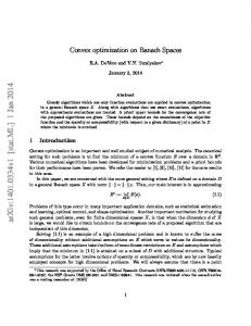
Fig. 1. The proposed relaxation method can approximate the solution to multi-labeling problems with a huge number of possible labels by globally solving a convex relaxation model. This example shows two images and the optic flow field between the two, where flow vectors were assigned from a possible set of 50 × 50 vectors, with truncated linear distance as a regularizer. The problem has so many different labels that a solution cannot be computed by alternative relaxation methods on current hardware. See Fig. 7 for the color code of the flow vectors.

The goal is to find a labeling g : Ω → Γ which minimizes the sum of the total costs and the regularizer, i.e. cg(x) (x) dx . (1) argmin J(g) + g∈L2 (Ω,Γ )

1.2

Ω

Discrete Approaches

It is well known that in the fully discrete setting, the minimization problem (1) is equivalent to maximizing a Bayesian posterior probability, where the prior probability gives rise to the regularizer [6]. The problem can be stated in the framework of Markov Random Fields [7] and discretized using a graph representation, where the nodes denote discrete pixel locations and the edges encode the energy functional [8]. Fast combinatorial minimization methods based on graph cuts can then be employed to search for a minimizer. In the case that the label space is binary and the regularizer submodular, a global solution of (1) can be found by computing a minimum cut [9,10]. For multi-label problems, one can approximate a solution for example by solving a sequence of binary problems (α-expansions) [11,12], or linear programming relaxations [13]. Exact solutions to multi-label problems can only be found in some special cases, notably [14], where a cut in a multilayered graph is computed in polynomial time to find a global optimum. The construction is restricted to convex iteraction terms with respect to a linearly ordered label set. However, in many important scenarios the label space can not be ordered, or a non-convex regularizer is more desireable to better preserve discontinuities in the solution. Even for relatively simple non-convex regularizers like the Potts distance, the resulting combinatorial problem is NP-hard [11]. Furthermore, it is known that the graph-based discretization induces an anisotropy, so that the

Convex Relaxation for Multilabel Problems with Product Label Spaces

227

solutions suffer from metrication errors [15]. It is therefore interesting to investigate continuous approaches as a possible alternative. 1.3

Continuous Approaches

Continuous approaches deal with the multi-label problem by transforming it into a continuous convex problem, obtaining the globally optimal solution, and projecting the continuous solution back onto the original discrete space of labels. Depending on the class of problem, it can be possible to obtain globally optimal solutions to the original discrete minimization problem. As in the discrete setting, it is possible to solve the two-label problem in a globally optimal way by minimizing a continuous convex energy and subsequent thresholding [2]. In the case of convex interaction terms and a linearly ordered set of labels, there also exists a continuous version of [14] to obtain globally optimal solutions [3]. For the general multi-label case, however, there is no relaxation known which leads to globally optimal solutions of the discrete problem. Currently the most tight relaxation is [4]. The theoretical basis of the reduction technique introduced in this paper is the slightly more transparent formulation introduced in [5] and further generalized in [1], but it can be easily adapted to the framework [4] as well. The convex relaxation described in [1,5] works as follows. Instead of looking for g directly, we associate each label γ with a binary indicator function uγ ∈ L2 (Ω, {0, 1}), where uγ (x) = 1 if and only if g(x) = γ. To make sure that a unique label is assigned to each point, only one of the indicator functions can have the value one. Thus, we restrict optimization to the space ⎧ ⎫ ⎨ ⎬ uγ (x) = 1 for all x ∈ Ω . UΓ := (uγ )γ∈Γ : uγ ∈ L2 (Ω, {0, 1}) and ⎩ ⎭ γ∈Γ

(2) Let ·, · denote the inner product on the Hilbert space L2 (Ω), then problem (1) can be written in the equivalent form uγ , cγ , (3) argmin J(u) + u∈UΓ

γ∈Γ

where we use bold face notation u for vectors (uγ )γ∈Γ indexed by elements in Γ . We use the same symbol J to also denote the regularizer on the reduced space. Its definition requires careful consideration, see Section 3. 1.4

Contribution: Product Label Spaces

In this work, we discuss label spaces which can be written as a product of a finite number d of discrete spaces, Γ = Λ1 × · · · × Λd . Let Nj be the number of elements in Λj , then the total number of labels is N = N1 · ... · Nd . In the formulation (3), we optimize over a number of N binary functions, which can

228

B. Goldluecke and D. Cremers Λ1 0

Γ 0

0

0

0

1

0

0

0

0

0 1 0 0 0

1

0

Λ2

Fig. 2. The central idea of the reduction technique is that if a single indicator function in the product space Γ takes the value 1, then this is equivalent to setting an indicator function in each of the factors Λj . The memory reduction stems from the fact that there are much more labels in Γ than in all the factors Λj combined.

be rather large in practical problems. In order to make problems of this form feasible to solve, we present a further reduction which only requires N1 +· · ·+Nd binary functions - a linear instead of an exponential growth. We will show that with our novel reduction technique, it is possible to efficiently solve convex relaxations to multi-label problems which are far too large to approach with previously existing techniques. A prototypical example is optic flow, where a typical total number of labels is around 322 for practical problems, for which we only require 64 indicator functions instead of 1024. However, the proposed method applies to a much larger class of labelling problems. A consequence of the reduction in variable size is a disproportionately large cut in required runtime, which also makes our method much faster.

2 2.1

Relaxations for Product Label Spaces Product Label Spaces

As previously announced, from now on we assume that the space of labels is a product of a finite number d of discrete spaces, Γ = Λ1 ×· · ·×Λd , with |Λj | = Nj . To each label λ ∈ Λj , 1 ≤ j ≤ d, we associate an indicator function ujλ . Thus, optimization will take place over the reduced space of functions

× UΓ := (ujλ )1≤j≤d,λ∈Λj : ujλ ∈ L2 (Ω, {0, 1}) and (4) j uλ (x) = 1 for all x ∈ Ω, 1 ≤ j ≤ d . λ∈Λj


1

229

co (m) = 0.05 = 0.15 = 0.20

0.8 0.6 0.4 0.2 0

(a) Product function m(x1 , x2 ) = x1 x2

0

0.5

1 x1 + x2

1.5

2

(b) Convex envelope co (m) and mollified versions for different

Fig. 3. Product function and its mollified convex envelope for the case d = 2

We use the short notation u× for a tuple (ujλ )1≤j≤d,λ∈Λj . Note that such a tuple consists indeed of exactly N1 + ... + Nd binary functions. The following proposition illuminates the relationship between the function spaces UΓ and UΓ× . Proposition 1. A bijection u× → u from UΓ× onto UΓ is defined by setting uγ := u1γ1 · ... · udγd , for all γ = (γ1 , ..., γd ) ∈ Γ . This is easy to see visually, Figure 2. A formal proof can be found in the appendix. With this new function space, another equivalent formulation to (1) and (3) is

argmin J(u× ) + u1γ1 · ... · udγd , cγ . (5) u× ∈UΓ×

γ∈Γ

Note that while we have reduced the dimensionality of the problem considerably, we have introduced another difficulty: the data term is not convex anymore, since it contains a product of the components. Thus, in the relaxation, we need to take additional care to make the final problem again convex. 2.2

Convex Relaxation

Two steps have to be taken to relax (5) to a convex problem. In a first step, we replace the multiplication function m(u1γ1 , ..., udγd ) := u1γ1 · ... · udγd with a convex function. In order to obtain a tight relaxation, we first move to the convex envelope co (m) of m. Analyzing the epigraph of m, Fig. 3(a) shows that 1 if x1 = ... = xd = 1, (6) co (m) (x1 , ..., xd ) = 0 if any xj = 0.

230


This means that if in the functional, m is replaced by the convex function co (m), we retain the same binary solutions, as the function values on binary input are the same. We lose nothing on first glance, but on second glance, we forfeited differentiability of the data term, since co (m) is not a smooth function anymore. In order to be able to solve the new problem in practice, we replace co (m) again by a mollified function co (m) , where > 0 is a small constant. We illustrate this for the case d = 2, where one can easily write down the functions explicitly. In this case, the convex envelope of multiplication is 0 if x1 + x2 ≤ 1 co (m) (x1 , x2 ) = x1 + x2 − 1 otherwise. This is a piecewise linear function of the sum of the arguments, i.e symmetric in x1 and x2 , see Fig. 3(b). We smoothen the kink by replacing co (m) with ⎧ ⎪ if x1 + x2 ≤ 1 − 4 ⎨0 1 2 co (m) (x1 , x2 ) = 16 (x1 + x2 − (1 − 4 )) if 1 − 4 < x1 + x2 < 1 + 4 ⎪ ⎩ 1 if x1 + x2 ≥ 1 + 4 This function does not satisfy the above condition (6) exactly, but only fulfills the less tight = 1 if x1 = · · · = xd = 1, co (m) (x1 , . . . , xd ) (7) ≤ if any xj = 0. The following Theorem shows that the solutions of the smoothened energy converge to the solutions of the original energy as → 0. After discretization, this means that we obtain an exact solution to the binary problem if we choose small enough, since the problem is combinatorial and the number of possible configurations finite. Theorem 1. Let > 0 and co (m) satisfy condition (7). Let u× 0 be a solution to problem (5), and

× u× co (m) (u1γ1 , ..., udγd ), cγ . (8) ∈ argmin J(u ) + u× ∈UΓ×

Then

γ∈Γ

× E (u×

cγ

) − E(u ) ≤ |Ω| 0

∞

,

(9)

γ∈Γ

where E and E are the energies of the original problem (5) and smoothened problem (8), respectively. The proof can be found in the appendix. The key difference of (8) compared to (5) is that the data term is now a convex function. In the second step of the convex relaxation, we have to make sure the domain of the optimization is a convex set. Thus UΓ× is replaced by its convex


231

hull co UΓ× . This just means that the domain of the functions (ujλ ) is extended to the continuous interval [0, 1]. The final relaxed problem which we are going to solve is now to find

argmin J(u× ) + co (m) (u1γ1 , ..., udγd ), cγ . (10) u× ∈co(UΓ× ) γ∈Γ 2.3

Numerical Method

With a suitable choice of convex regularizer J, problem (10) is a continuous convex problem with a convex and differentiable data term. In other relaxation methods, one usually employs fast primal-dual schemes [16,17] to solve the continuous problem. However, those are only applicable to linear data terms. Fortunately, the derivative of the data term is Lipschitz-continuous with Lipschitz 1

c

constant L = 8 γ 2 . If we take care to choose a lower semi-continuous J, γ we are thus in a position to apply the FISTA scheme [18] to the minimization of (10). It is much faster than for example direct gradient descent, with a provable quadratic convergence rate. The remaining problems are how to choose a correct regularizer, and how to get back from a possibly non-binary solution of the relaxed problem to a solution of the original problem. 2.4

Obtaining a Solution to the Original Problem

ˆ × be a solution to the relaxed problem (10). Thus, the functions u ˆjλ might Let u have values in between 0 and 1. In order to obtain a feasible solution to the original problem (1), we just project back to the space of allowed functions. The ˆ × is given by setting function gˆ ∈ L2 (Ω, Γ ) closest to u gˆ(x) = argmax uˆ1γ1 (x) · ... · uˆdγd (x) , γ∈Γ

i.e. we choose the label where the combined indicator functions have the highest value. We cannot guarantee that the solution gˆ is indeed a global optimum of the original problem (1), since there is nothing equivalent to the thresholding theorem [2] known for this kind of relaxation. However, we still can give a bound how close we are to the global optimum. Indeed, the energy of the optimal solution ˆ × and gˆ. of (1) must lie somewhere between the energies of u

3

Regularization

The following construction of a family of regularizers is analogous to [1], but extended to accomodate product label spaces. An element u× ∈ UΓ× can be viewed as a map in L2 (Ω, Δ× ), where Δ× = Δ1 × ... × Δd ⊂ RN1 +...+Nd

232


and Δi =

⎧ ⎨ ⎩

x ∈ {0, 1}Ni :

Ni

⎫ ⎬ xj = 1

j=1

⎭

.

is the set of corners of the standard (k − 1)-simplex. As shown previously, there is a one-to-one correspondence between elements in Δ× and labels in Γ . the We will now construct a familiy of regularizers J : co UΓ× → R and afterwards demonstrate that it is well suited to the problem at hand. For this, we impose a metric d on the space Γ of labels. A current limitation is that we can only handle the case of separable metrics, i.e. d must be of the form d(γ, χ) =

d

di (γi , χi ),

(11)

i=1

where each di is a metric on Δi . We further assume that each di has an Euclidean representation. This means that each label λ ∈ Δi shall be represented by an ri dimensional vector aiλ ∈ Rri , and the distance di defined as Euclidean distance between the representations, d(λ, μ) = |aλ − aμ |2 for all λ, μ ∈ Δi .

(12)

The goal in the construction of J is that the higher the distance between labels, the higher shall be the penalty imposed by J. To make this idea precise, we introduce the linear mappings Ai : co Δi → Rri which map labels onto their representations, Ai (λ) = aiλ for all λ ∈ Δi . When the labels are enumerated, then in matrix notation, the vectors aiγ become exactly the columns of Ai , which shows the existence of this map. We can now define the regularizer as J(u× ) :=

d

TViv (Ai ui ) ,

(13)

i=1

where TViv is the vectorial total variation on L2 (Ω, Rri ). The following theorem shows why the above definition makes sense. Theorem 2. The regularizer J defined in (13) has the following properties: 1. J is convex and positively homogenous on co UΓ× . 2. J(u× ) = 0 for any constant labeling u× . 3. If S ⊂ Ω has finite perimeter Per(S), then for all labels γ, χ ∈ Γ , J(γ1S + χ1S c ) = d(γ, χ) Per(S) , i.e. a change in labels is penalized proportional to the distance between the labels and the perimeter of the interface.


233

The theorem is proved in the appendix. More general classes of metrics on the labels can also be used, see [1]. For the sake of simplicity, we only included the most important example of distances with Euclidean representations. This class includes, but is not limited to, the following special cases: – The Potts or uniform distance, where di (λ, μ) = 1 if and only if λ = μ, and zero otherwise. This distance function can be achieved by setting aiλ = 12 eλ , where (eλ )λ∈Λi is an orthonormal basis in RNi . All changes between labels are penalized equally. – The typical case is that the aiλ denote feature vectors or actual geometric points, for which |·|2 is a natural distance. For example, in the case of optic flow, each label corresponds to a flow vector in R2 . The representations a1λ , a2μ are just real numbers, denoting the possible components of the flow vectors in x and y-direction, respectively. The Euclidean distance is a natural distance on the components to regularize the flow field, corresponding to the regularizer of the TV-L1 functional in [19]. The convex functional we wish to minimize is now fully defined, including the regularizer. The ROF type problems with the vectorial total variation as a regularizer, which are at the core of the resulting FISTA scheme, can be minimized with algorithms in [20]. For the also required backprojections onto simplices we recommend the method in [21]. Thus, we can turn our attention towards computing a minimizer in practice. In the remaining section, we will apply the framework to a variety of computer vision problems.

4

Experiments

We implemented the proposed algorithm for the case d = 2 on parallel processing GPU architecture using the CUDA programming language, and performed a variety of experiments, with completely different data terms and regularizers. All experiments were performed on an nVidia Tesla C1060 card with 4GB of memory. When the domain Ω is discretized into P pixels, the primal and dual variables required for the FISTA minimization scheme are represented as matrices. In total, we have to store P · (N1 + ... + Nd ) floating point numbers for the primal variables, and P n · (r1 + ... + rd ) floating point numbers for the dual variables. In contrast, without using our reduction scheme, this number would be as high as P · N1 · ... · Nd for the primal variables and P n · r1 · ... · rd for the dual variables, respectively. For the FISTA scheme, we need space for four times the primal variables in total, so we end up with the total values shown in Fig. 4. Thus, problems with large number of labels can only be handled with the proposed reduction technique. 4.1

Multi-label Segmentation

For the first example, we chose one with a small label space, so that we can compare the convergence rate and solution energy of the previous method [1]

234


3 # Labels Memory [Mb] Runtime [s] N1 × N2 Previous Proposed Previous Proposed 8×8 112 28 196 6 16 × 16 450 56 ∗ 21 32 × 32 1800 112 ∗ 75 64 × 64 7200 225 314 8×8 448 112 789 22 16 × 16 1800 224 ∗ 80 32 × 32 7200 448 297 64 × 64 28800 900 1112

2.5 Energy

# of Pixels P = Px × Py 320 × 240 320 × 240 320 × 240 320 × 240 640 × 480 640 × 480 640 × 480 640 × 480

Proposed Previous

2

1.5 1

0.5 0

0 2 4 6 8 10 12 14 Iteration

Fig. 4. The table shows the total amount of memory required for a FISTA implementation of the previous and proposed methods depending on the size of the problem. Also shown is the total runtime for 15 iterations, which usually suffices for convergence. Numbers shown in red cannot be stored within even the largest of todays CUDA capable cards, so an efficient parallel implementation is not possible. Failures marked with a “∗” are due to another limitation: the shared memory is only sufficient to store the temporary variables for the simplex projection up until dimension 128. In the graph, we see a comparison of the convergence rate between the original scheme and the proposed scheme. Despite requiring significantly less memory and runtime, the relaxation is still sufficiently tight to arrive at an almost similar solution.

with the proposed one. We perform a segmentation of an image based on the HSL color space. The hue and lightness values of the labeling are taken from the discrete sets of equidistant labels Λ1 and Λ2 , respectively. Their size is |Λ1 | = |Λ2 | = 8, so there are 64 labels in total, which can still be handled by the old method as well, albeit barely. The labels shall be as close as possible to the original image values, so the cost function penalizes the L1 -distance in HSV color space. We choose the regularizer so that the penalty for discontinuities is proportionally larger in regions with higher lightness. The relaxation constant is reduced from 0.2 to 0.05 during the course of the iterations. The result can be seen in Fig. 5, while a comparison of the respective convergence rates are shown in the graph in Fig. 4. The proposed method, despite requiring only a fraction of the memory and computation time, achieves a visually similar result with only a slightly higher energy. Note that the runtime of our method is far lower, since the simplex projection becomes disproportionally more expensive if the length of the vector is increased. 4.2

Depth and Occlusion Map

In this test, we simultaneously compute a depth map and an occlusion map for a stereo pair of two color input images IL , IR : Ω → R3 . The occlusion map shall be a binary map denoting wether a pixel in the left image has a matching pixel in the right image. Thus, the space of labels is two-dimensional with Λ1 consisting of the disparity values and a binary Λ2 for the occlusion map. We use the technique in [1] to approximate a truncated linear smoothness penalty on


235

Fig. 5. Results for the multi-label segmentation. The input image on the left was labelled with 8 × 8 labels in the hue and lightness components of HSL color space. The label distance is set so that smoothing is stronger in darker regions, which creates an interesting visual effect.

Fig. 6. The proposed method can be employed to simultaneously optimize for a displacement and an occlusion map. This problem is also too large to be solved by alternative relaxation methods on current GPUs. From left to right: (a) Left input image IL . (b) Right input image IR . (c) Computed disparity and occlusion map, red areas denote occluded pixels.

the disparity values. A Potts regularizer is imposed for the occlusion map. The distance on the label space thus becomes d(γ, χ) = s1 min(t1 , |γ1 − χ1 |) + s2 |γ2 − χ2 | ,

(14)

with suitable weights s1 , s2 > 0 and threshold t1 > 0. We penalize an occluded pixel with a constant cost cocc > 0, which corresponds to a threshold for the similarity measure above which we believe that a pixel is not matched correctly anymore. The cost associated with a label γ at (x, y) ∈ Ω is then defined as cocc if γ2 = 1, (15) cγ (x, y) =

IL (x, y) − IR (x − λ1 , y) 2 otherwise. The result for the “Moebius” test pair from the Middlebury benchmark is shown in Fig. 6. The input image resolution was scaled to 640 × 512, requiring 128 disparity labels, which resulted in a total memory consumption which was slightly too big for previous methods, but still in reach of the proposed algorithm. Total computation time required was 597 seconds.

236


First image I0

Second image I1

Flow field and color code

Fig. 7. When employed for optic flow, the proposed method can successfully capture large displacements without the need for coarse-to-fine approaches, since a global optimization is performed over all labels. In contrast to existing methods, our solution is within a known bound of the global optimum.

4.3

Optic Flow

In the final test, we compute optic flow between two color input images I0 , I1 : Ω → R3 taken at two different time instants. The space of labels is again twodimensional, with Λ1 = Λ2 denoting the possible components of flow vectors in x and y-direction, respectively. We regularize both directions with a truncated linear penalty on the component distance, i.e. d(γ, χ) = s min(t, |γ1 − χ1 |) + s min(t, |γ2 − χ2 |) ,

(16)

with a suitable weight s > 0 and threshold t > 0. The cost function just compares pointwise pixel colors in the images, i.e. cγ (x, y) = I0 (x, y) − I1 (x + γ1 , y + γ2 ) 2 .

(17)

Results can be observed in Fig. 1 and 7. Due to the global optimization of a convex energy, we can successfully capture large displacements without having to implement a coarse-to-fine scheme. The number of labels is 50×50 at an image resolution of 640×480, so the memory requirements are so high that this problem is currently impossible to solve with previous convex relaxation techniques by a large margin, see Fig. 4. Total computation time using our method was 678 seconds. A comparison of the energies of the continuous and discretized solution shows that we are within 5% of the global optimum for all examples.

5

Conclusion

We have introduced a continuous convex relaxation for multi-label problems where the label space is a product space. Such labeling problems are plentiful in computer vision. The proposed reduction method improves on previous methods in that it requires orders of magnitude less memory and computation time, while retaining the advantages: a very flexible choice of distance on the label space, a globally optimal solution of the relaxed problem and an efficient parallel GPU implementation with guaranteed convergence.


237

Because of the reduced memory requirements, we can successfully handle specific problems with very large number of labels, which could not be attempted with previous convex relaxation techniques. Among other examples we presented a convex relaxation for the optic flow functional with truncated linear penalizer on the distance between the flow vectors. To our knowledge, this is the first relaxation for this functional which can be optimized globally and efficiently.

References 1. Lellmann, J., Becker, F., Schn¨ orr, C.: Convex optimization for multi-class image labeling with a novel family of total variation based regularizers. In: IEEE International Conference on Computer Vision (ICCV) (2009) 2. Nikolova, M., Esedoglu, S., Chan, T.: Algorithms for finding global minimizers of image segmentation and denoising models. SIAM Journal of Applied Mathematics 66, 1632–1648 (2006) 3. Pock, T., Schoenemann, T., Graber, G., Bischof, H., Cremers, D.: A convex formulation of continuous multi-label problems. In: Forsyth, D., Torr, P., Zisserman, A. (eds.) ECCV 2008, Part III. LNCS, vol. 5304, pp. 792–805. Springer, Heidelberg (2008) 4. Pock, T., Chambolle, A., Bischof, H., Cremers, D.: A convex relaxation approach for computing minimal partitions. In: IEEE Conference on Computer Vision and Pattern Recognition (CVPR), pp. 810–817 (2009) 5. Zach, C., Gallup, D., Frahm, J., Niethammer, M.: Fast global labeling for realtime stereo using multiple plane sweeps. In: Vision, Modeling and Visualization, pp. 243–252 (2009) 6. Szeliski, R.: Bayesian modeling of uncertainty in low-level vision. International Journal of Computer Vision 5, 271–301 (1990) 7. Kindermann, R., Snell, J.: Markov Random Fields and Their Applications. American Mathematical Society, Providence (1980) 8. Boykov, Y., Kolmogorov, V.: Computing geodesics and minimal surfaces via graph cuts. In: IEEE International Conference on Computer Vision (ICCV), pp. 26–33 (2003) 9. Greig, D., Porteous, B., Seheult, A.: Exact maximum a posteriori estimation for binary images. J. Royal Statistics Soc. 51, 271–279 (1989) 10. Kolmogorov, V., Zabih, R.: What energy functions can be minimized via graph cuts. IEEE Trans. Pattern Anal. Mach. Intell. 26, 147–159 (2004) 11. Boykov, Y., Veksler, O., Zabih, R.: Fast approximate energy minimization via graph cuts. IEEE Trans. Pattern Anal. Mach. Intell. 23, 1222–1239 (2001) 12. Schlesinger, D., Flach, B.: Transforming an arbitrary min-sum problem into a binary one. Technical report, Dresden University of Technology (2006) 13. Wainwright, M., Jaakkola, T., Willsky, A.: Map estimation via agreement on trees: message-passing and linear programming. IEEE Trans. Inf. Theory 51, 3697–3717 (2005) 14. Ishikawa, H.: Exact optimization for markov random fields with convex priors. IEEE Trans. Pattern Anal. Mach. Intell. 25, 1333–1336 (2003) 15. Klodt, M., Schoenemann, T., Kolev, K., Schikora, M., Cremers, D.: An experimental comparison of discrete and continuous shape optimization methods. In: Forsyth, D., Torr, P., Zisserman, A. (eds.) ECCV 2008, Part I. LNCS, vol. 5302, pp. 332–345. Springer, Heidelberg (2008) 16. Popov, L.: A modification of the arrow-hurwicz method for search of saddle points. Math. Notes 28, 845–848 (1980)

238


17. Nesterov, Y.: Smooth minimization of non-smooth functions. Math. Prog. 103, 127–152 (2004) 18. Beck, A., Teboulle, M.: Fast iterative shrinkage-thresholding algorithm for linear inverse problems. SIAM J. Imaging Sciences 2, 183–202 (2009) 19. Zach, C., Pock, T., Bischof, H.: A duality based approach for realtime T V − L1 optical flow. In: Hamprecht, F.A., Schn¨ orr, C., J¨ ahne, B. (eds.) DAGM 2007. LNCS, vol. 4713, pp. 214–223. Springer, Heidelberg (2007) 20. Duval, V., Aujol, J.F., Vese, L.: Projected gradient based color image decomposition. In: Tai, X.-C., Mørken, K., Lysaker, M., Lie, K.-A. (eds.) Scale Space and Variational Methods in Computer Vision. LNCS, vol. 5567, pp. 295–306. Springer, Heidelberg (2009) 21. Michelot, C.: A finite algorithm for finding the projection of a point onto the canonical simplex of Rn . J. Optimization Theory and Applications 50, 195–200 (1986)

Appendix Proof of Proposition 1. In order to proof the proposition, we have to show that the mapping induces a point-wise bijection from Δ× onto ⎫ ⎧ N ⎬ ⎨ xj = 1 . Δ = x ∈ {0, 1}N : ⎭ ⎩ j=1

We first show it is onto: for u(x) in Δ, there exists exactly one γ ∈ Γ with uγ (x) = 1. Set uiλ (x) = 1 if λ = γi , and uiλ (x) = 0 otherwise. Then u(x) = u1 (x) · ... · ud (x), as desired. To see that the map is one-to-one, we just count the elements in Δ× . Since Δi contains Ni elements, the number of elements in Δ× is N1 · ... · Nd = N , the same as in Δ. Proof of Theorem 1. The regularizers of the original and smoothened problems are the same, so because of condition (7), × E (u× ≤ |Ω| ) − E(u ) c dx

cγ ∞ . (18) ≤ γ 0 γ∈Γ Ω γ∈Γ

This completes the proof.

Proof of Theorem 2. The first two claims are basic properties of the total variation. For the last claim, we combine Corollary 1 in [1] with the definition of the metric in equations (11) and (12) to find J(γ1S + χ1S c ) =

d

TViv (Ai (γ1S + χ1S c )) =

i=1

d i aγ − aiχ Per(S) 2 i=1

(19)

= d(γ, χ) Per(S). This completes the proof.