Feb 22, 2016 - arXiv:1602.06746v1 [cs.LG] 22 Feb 2016. Convexification of Learning from Constraints. Iaroslav Shcherbatyi. [email protected].
Convexification of Learning from Constraints Iaroslav Shcherbatyi
SHCHERBATYI @ MPI - INF. MPG . DE
Max Planck Institute for Informatics, Saarbr¨ucken, Germany
Bjoern Andres
ANDRES @ MPI - INF. MPG . DE
arXiv:1602.06746v1 [cs.LG] 22 Feb 2016
Max Planck Institute for Informatics, Saarbr¨ucken, Germany
Abstract Regularized empirical risk minimization with constrained labels (in contrast to fixed labels) is a remarkably general abstraction of learning. For common loss and regularization functions, this optimization problem assumes the form of a mixed integer program (MIP) whose objective function is non-convex. In this form, the problem is resistant to standard optimization techniques. We construct MIPs with the same solutions whose objective functions are convex. Specifically, we characterize the tightest convex extension of the objective function, given by the Legendre-Fenchel biconjugate. Computing values of this tightest convex extension is NP-hard. However, by applying our characterization to every function in an additive decomposition of the objective function, we obtain a class of looser convex extensions that can be computed efficiently. For some decompositions, common loss and regularization functions, we derive a closed form.
1. Introduction We study an optimization problem: Given a finite set S 6= ∅ whose elements are to be labeled as 0 or 1, a non-empty set Y ⊆ {0, 1}S of feasible labelings, x : S → Rm with m ∈ N, called a feature matrix, l : R×[0, 1] → R+ 0 with l(·, 0) convex, l(·, 1) convex, l(r, 1) → 0 as r → ∞ and l(−r, 0) → 0 as r → ∞, called a loss function, Θ ⊆ Rm convex, called the set of feasible parameters, ω : Θ → + R+ 0 convex, called a regularization function, and C ∈ R0 , called a regularization constant, we consider the optimization problem inf
(θ,y)∈Θ×Y
ϕ(θ, y)
with ϕ(θ, y) := ω(θ) +
C X ls (θ, ys ) |S|
(1)
(2)
s∈S
ls (θ, ys ) := l(hxs , θi, ys ) .
(3)
ˆ xi) and ˆ yˆ), if it exists, defines a classifier c : Rm → {0, 1} : x 7→ 1 (1 + sgn hθ, A minimizer (θ, 2 a feasible labeling yˆ ∈ Y . The optimization problem (1) is a remarkably general abstraction of learning. On the one hand, it generalizes supervised, semi-supervised and unsupervised learning: • If the labeling y is fixed by |Y | = 1 to precisely one feasible labeling, (1) specializes to regularized empirical risk minimization with fixed labels and is called supervised. • If Y fixes the label of at least one but not all elements of S, (1) is called semi-supervised. • If Y constrains the joint labelings of S without fixing the label of any Psingle element of S, (1) is called unsupervised. For example, consider Y = {y ∈ {0, 1}S | s∈S ys = ⌊|S|/2⌋}. 1
S HCHERBATYI A NDRES
On the other hand, the optimization problem (1) generalizes classification, clustering and ranking: • If S = A × B and Y is the set of characteristic functions of maps from A to B, (1) is an abstraction of multi-label classification, as discussed, for instance, by Joachims (1999, 2003); Chapelle and Zien (2005); Xu and Schuurmans (2005); Chapelle et al. (2006b,a, 2008). • If S = A × A and Y is the set of characteristic functions of equivalence relations on A, (1) is an abstraction of clustering, as discussed by Finley and Joachims (2005); Xu et al. (2005). For fixed parameters θ, it specializes to the NP-hard minimum cost clique partition problem (Gr¨otschel and Wakabayashi, 1989; Chopra and Rao, 1993) that is also known as correlation clustering (Bansal et al., 2004; Demaine et al., 2006). • If S = A × A and Y is the set of characteristic functions of linear orders on A, (1) is an abstraction of ranking. For fixed parameters θ, it specializes to the NP-hard linear ordering problem (Mart´ı and Reinelt, 2011). The set Y of feasible labelings, a subset of the vertices of the unit hypercube [0, 1]S , is a nonconvex subset of RS iff 2 ≤ |Y |. Typically, one considers a relaxation y ∈ P of the constraint y ∈ Y with P a convex polytope such that conv Y ⊆ P ⊆ [0, 1]S and P ∩ {0, 1}S = Y . In practice, one considers a polytope that is described as an intersection of half-spaces, i.e., by n ∈ N, A ∈ Rn×S and b ∈ Rn such that P = {y ∈ RS | Ay ≤ b}. Also typically, the set Θ ⊆ Rm of feasible parameters is a convex polyhedron and is described also as an intersection of half-spaces, ′ ′ i.e., by n′ ∈ N, A′ ⊆ Rn ×m and b′ ∈ Rn such that Θ = {θ ∈ Rm | A′ θ ≤ b′ }. Hence, the optimization problem (1) assumes the form of a mixed integer program (MIP): inf
(θ,y)∈Rm ×[0,1]S
subject to
ϕ(θ, y)
(4)
A′ θ ≤ b′
(5)
Ay ≤ b
(6) S
y ∈ {0, 1}
(7)
For convex loss functions ls such as the squared difference loss (Tab. 1), the objective function ϕ is convex on the domain Rm × [0, 1]S . Thus, the continuous relaxation (4)–(6) of the problem (4)–(7) is a convex problem. Its solutions (θˆ′ , yˆ′ ), although possibly fractional in the coordinates of y ′ , can inform a search for feasible solutions of (4)–(7) with certificates (Chapelle et al., 2006b, 2008; Bojanowski et al., 2013). See also Bonami et al. (2012) for a recent survey of convex mixedinteger non-linear programming. For non-convex loss functions ls such as the logistic loss, the Hinge loss and the squared Hinge loss (Tab. 1), ϕ is non-convex on the domain Rm × [0, 1]S . In this case, (4)–(7) is resistant to standard optimization techniques. See Tawarmalani and Sahinidis (2004); Lee and Leyffer (2011); Belotti et al. (2013) for an overview of non-convex mixed-integer non-linear programming. Table 1: Loss functions Loss
Form of ls (θ, ys )
Function ls : Rm × [0, 1] → R+ 0
Squared difference Logistic Hinge Squared Hinge
(hθ, xs i − ys )2 log(1 + exp(−(2ys − 1)hθ, xs i)) max{0, 1 − (2ys − 1)hθ, xs i} max{0, 1 − (2ys − 1)hθ, xs i}2
convex non-convex non-convex non-convex
2
C ONVEXIFICATION
OF
L EARNING
C ONSTRAINTS
FROM
20
20
20
10
10
10
1
0 1
1
y 0.5 0
−2
0
2 θ
y 0.5 0
(a)
−2
0
2 θ
(b)
y 0.5 0
−2
0
2 θ
(c)
Figure 1: Depicted above in (a) is the non-convex objective function ϕ of the optimization problem (1) for Y = {0, 1}, Θ = R, the Hinge loss (Tab. 1) and ω(·) = k · k22 . Its restriction φ to the feasible set Θ × {0, 1} is depicted in black. As the goal is to minimize ϕ over the feasible set, one can replace the values of ϕ for y ∈ (0, 1) without affecting the solution, for instance, by zero, as depicted in (b). In this paper, we characterize the tightest convex extension of φ to Θ × conv Y , which is depicted in (c).
1.1. Contribution We construct, for the MIP (4)–(7) whose objective function is non-convex, MIPs with the same solutions whose objective functions are convex. Our approach is illustrated in Fig. 1 and is summarized below. In Section 3, we consider the restriction φ of ϕ to the feasible set Θ × Y and characterize the tightest convex extension φ∗∗ of φ to Θ × conv Y . This tightest convex extension φ∗∗ is mostly of theoretical interest as computing its values is NP-hard. In Section 4, we consider a decomposition of the function φ into a sum of functions. By applying our characterization of tightest convex extensions to every function in this sum, we construct a convex extension φ′ of φ to Θ × [0, 1]S which is not generally tight but whose values can be computed efficiently. For common loss and regularization functions, we derive a closed form. For every convex extension φ′ we construct, including φ∗∗ , the MIP φ′ (θ, y)
inf
(θ,y)∈Rm ×RS
(8)
subject to A′ θ ≤ b′
(9)
Ay ≤ b
(10) S
y ∈ {0, 1}
(11)
has the same solutions as (4)–(7). Like (4)–(7), it is NP-hard, due to the integrality constraint (11). Unlike (4)–(7), its objective function and polyhedral relaxation (8)–(10) are convex. Thus, unlike (4)–(7), it is accessible to a wide range of standard optimization techniques.
3
S HCHERBATYI A NDRES
2. Related Work 2.1. Convex Extensions For large classes of univariate and bivariate functions, tightest convex extensions have been characterized by Tawarmalani et al. (2013) and Locatelli (2014). Convex envelopes of multivariate functions that are convex in all but one variable have been characterized by Jach et al. (2008). For functions of the form f (x, y) = g(x)h(y) and with g and h having additional properties, e.g., g being component-wise concave and submodular, and h being univariate convex, tightest convex extensions have been characterized by Khajavirad and Sahinidis (2012, 2013). For functions f : A × B → R with A, B ⊆ Rn and f (a, ·) being either convex or concave and f (·, b) being either convex or concave for any a ∈ A and b ∈ B, tightest convex extensions have been characterized by Ballerstein (2013). Tightest convex extensions of pseudo-Boolean functions f : {0, 1}n → R are known as convex closures (Bach, 2013). Convex closures of submodular functions are Lov´asz extensions. The characterization of tightest convex extensions of functions f : Θ × Y → R with f (·, y) convex for all y ∈ Y that we establish is consistent with results of Jach et al. (2008) for functions f : Rn × {0, 1} → R. It extends some results of Jach et al. (2008) to non-differentiable f (·, 0) and f (·, 1). 2.2. Regularized Empirical Risk Minimization with Constrained Labels Regularized empirical risk minimization with constrained labels has been studied intensively in the special case of semi-supervised learning for 01-classification. Algorithms that find feasible solutions efficiently are due to Joachims (1999, 2003); Chapelle and Zien (2005); Chapelle et al. (2006a,b); Sindhwani et al. (2006). A branch-and-bound algorithm that solves the problem to optimality was suggested by Vapnik and Chervonenkis (1974) and has been implemented and applied to data by Chapelle et al. (2006b, 2008), with the result that optimal solutions generalize better typically than feasible solutions found by approximate algorithms. An approach to the problem by convex optimization, specifically, by a semi-definite relaxation of the dual problem, was proposed by Bie and Cristianini (2006). Similar relaxations have been studied in the context of semi-supervised learning for multi-label classification (Xu and Schuurmans, 2005; Guo and Schuurmans, 2011), correlation clustering (Xu et al., 2005; Zhang et al., 2009) and latent variable estimation (Guo and Schuurmans, 2008). For maximum margin clustering, a convex relaxation tighter than the SDP relaxation is constructed by Li et al. (2009). For multi-label classification with a softmax loss function, a tight SDP relaxation is proposed by Joulin and Bach (2012).
4
C ONVEXIFICATION
OF
L EARNING
FROM
C ONSTRAINTS
3. Tightest Convex Extensions In this section, we consider the restriction φ of ϕ to the feasible set Θ × Y , i.e., the function φ:
Θ × Y → R+ 0 :
(θ, y) 7→ ϕ(θ, y) .
(12)
We characterize the tightest convex extension φ∗∗ of φ to Θ × conv Y in Theorem 3. Definition 1 (Tawarmalani and Sahinidis, 2002) For any n ∈ N, any A ⊆ Rn and any φ : A → R, a function φ′ : conv A → R is called a convex extension of φ iff φ′ is convex and ∀a ∈ A : φ′ (a) = φ(a). Moreover, a function φ∗∗ : conv A → R is called the tightest convex extension of φ iff φ∗∗ is a convex extension of φ and, for every convex extension φ′ of φ and for all a ∈ conv A: φ′ (a) ≤ φ∗∗ (a). Lemma 2 A (tightest) convex extension φ∗∗ of φ exists. Theorem 3 For every finite S 6= ∅, every Y ⊆ {0, 1}S with |Y | > |S|, every m ∈ N, every convex Θ ⊆ Rm and every φ : Θ × Y → R+ 0 such that φ(·, y) is convex for every y ∈ Y , the tightest convex extension φ∗∗ : Θ × conv Y → R+ 0 of φ is such that for all (θ, y) ∈ Θ × conv Y : ) ( X X (13) λ ′ (y ′ ) θ ′ (y ′ ) = θ λyY ′ (y ′ ) φ(θ ′ (y ′ ), y ′ ) φ∗∗ (θ, y) = min ′ inf ′ ′ yY Y ′ ∈Y(y) θ :Y ′ →Θ ′ ′ y ∈Y
y ∈Y
where
n
′
Y(y) := Y ∈
Y � |S|+1
o y ∈ conv Y ′
(14)
is the set of (|S| + 1)-elementary subsets Y ′ of Y having y in their convex hull, and, for every y ∈ conv Y and every Y ′ ∈ Y(y): λyY ′ : Y ′ → R+ 0 are the coefficients in the convex combination of y in Y ′ , i.e. X (15) λyY ′ (y ′ ) y ′ = y y ′ ∈Y ′
X
λyY ′ (y ′ ) = 1 .
(16)
y ′ ∈Y ′
Remarks are in order: • |Y(y)| can be strongly exponential in |S|. This is expected, given that the complexity of computing the value of a convex extension is NP-hard. • Given a polynomial-time oracle for the outer minimization in (13), the tightest convex extension can be computed in polynomial time. • Conceivable is a polynomial-time oracle for constraining Y(y) to a strict subset without compromising optimality in (13). • An upper bound on the tightest convex extension can be obtained by considering any subset of Y(y). 5
S HCHERBATYI A NDRES
10
10
10
5
5
5
1
1
1
y 0.5
0
−2
0
2
y 0.5
θ
(a)
0
−2
0
2
y 0.5
θ
(b)
0
−2
0
2 θ
(c)
Figure 2: Depicted above in (a) is the non-convex objective function ϕ of the optimization problem (1) for Y = {0, 1}, Θ = R, the Hinge loss (Tab. 1) and ω(·) = k · k1 . Its restriction φ to Θ × {0, 1} is depicted in black. Depicted in (b) is the tightest convex extension of φ to Θ × [0, 1]. Depicted in (c) is the tightest convex extension of φ to [−b, b] × [0, 1], for b ∈ R+ 0 . It can be seen that, for bounded θ, the tightest convex extension is continuous.
4. Efficient Convex Extensions In this section, we characterize, for common loss and regularization functions, convex extensions φ′ of φ that are not necessarily tight but can be computed efficiently in general. The construction is in two steps: Firstly, we consider an additive decomposition of φ. Specifically, we consider a convex function + c : Θ → R+ 0 and, for every s ∈ S, a function ds : Θ × {0, 1} → R0 such that ds (·, 0) and ds (·, 1) are convex. These functions are chosen such that, for all (θ, y) ∈ Θ × Y : 1 X ds (θ, ys ) . (17) φ(θ, y) = c(θ) + |S| s∈S
One example is given by c := ω and, for every s ∈ S, ds := C ls . Another example is given by c := 0 and, for every s ∈ S, every θ ∈ Θ and every ys ∈ {0, 1}: ds (θ, ys ) := ω(θ) + Cls (θ, ys ). Secondly, we characterize, for each ds , its tightest convex extension d∗∗ s : Θ × [0, 1] → R, by a specialization of Theorem 3 stated as Corollary 4. A convex extension φ′ of φ to Θ × [0, 1]S is then given by 1 X ∗∗ ds (θ, ys ) . (18) φ′ : Θ × [0, 1]S → R+ : (θ, y) → 7 c(θ) + 0 |S| s∈S
Corollary 4 For every d : Θ × {0, 1} → R+ 0 such that d0 (·) := d(·, 0) and d1 (·) := d(·, 1) are ∗∗ convex, the tightest convex extension d : Θ × [0, 1] → R+ 0 of d is such that for all (θ, y) ∈ Θ × Y : ( d(θ, y) if y ∈ {0, 1} (19) d∗∗ (θ, y) = Ψ(θ, y) if y ∈ (0, 1) with Ψ(θ, y) =
inf
θ 0 ,θ 1 ∈Θ
� (1 − y)d0 (θ 0 ) + yd1 (θ 1 ) (1 − y)θ 0 + yθ 1 = θ . 6
(20)
C ONVEXIFICATION
OF
L EARNING
FROM
C ONSTRAINTS
The solutions of the optimization problem (20) are characterized in Lemma 5. Subgradients are given in Lemma 6. Lemma 5 For every solution (θˆ0 , θˆ1 ) ∈ Θ2 of (20), there exists a G 6= ∅ such that, for ξθ,y : Θ → Θ : t 7→ (θ − (1 − y)t)/y: \ (δd0 )(θˆ0 ) (δd1 )(ξθ,y (θˆ0 )) = G (21) \ (δd0 )(ξθ,1−y (θˆ1 )) (δd1 )(θˆ1 ) = G . (22)
� Lemma 6 If a solution (θˆ0 , θˆ1 ) ∈ Θ2 of (20) exists, then wv ∈ (δd∗∗ )(θ, y) iff v ∈ G with G defined equivalently in (21) and (22) and w = v T θˆ0 − v T θˆ1 + d1 (θˆ1 ) − d0 (θˆ0 ). Otherwise, y ∈ {0, 1} and: � v y = 0 ⇒ ∀v ∈ (δd(·, 0))(θ) : ∞ ∈ (δd∗∗ )(θ, y) (23) � v ∗∗ y = 1 ⇒ ∀v ∈ (δd(·, 1))(θ) : −∞ ∈ (δd )(θ, y) . (24)
We proceed as follows: In Section 4.1, we consider two decompositions of the class (17) for which the tightest convex extension of any ds is easy to characterize but the resulting convex extension of φ is rather loose. In Sections 4.2 and 4.3, we consider decompositions of the class (17) with c = 0. These yield the tightest convex extension of φ of any decomposition of the class (17). For any combination of the logistic loss, the Hinge loss and the squadred Hinge loss (Tab. 1) with either L1 regularization ω(·) = k · k1 or L2 regularization ω(·) = k · k22 , we characterize the convex extension explicitly and, in some cases, in closed form. Examples of all combinations are depicted in Fig. 3. 4.1. Instructive Examples The first convex extension we characterize is for the decomposition (17) with c := ω and ∀s ∈ S : ds := Cls . Corollary 7 For any d : Θ×{0, 1} → R+ 0 such that d0 (·) := d(·, 0) and d1 (·) := d(·, 1) are convex and for which d0 (−r) → 0 and d1 (r) → 0 as r → ∞, the convex extension d∗∗ : Θ × [0, 1] → R of d has the form ( d(θ, y) if y ∈ {0, 1} . (25) d′ (θ, y) = 0 if y ∈ (0, 1) The second convex extension we characterize is for the logistic loss ls (θ, y) = −hx, θiy + log(1 + ehx,θi ), for ω(·) = k · k22 and for the decomposition (17) such that, for every s ∈ S, ds (θ, y) := kθk22 − Chx, θiy. + Corollary 8 The tightest convex extension d∗∗ : Θ × [0, 1] → R+ 0 of d : Θ × {0, 1} → R0 with C C 2 2 2 ∗∗ d(θ, y) = kθk2 − Chx, θiy has the form d (θ, y) = ||θ − y 2 x||2 − yk 2 xk2 .
7
S HCHERBATYI A NDRES
4.2. L2 Regularization We now consider ω(·) = 21 k · k22 and decompositions (17) such that, for every s ∈ S: ds (θ, y) = ω(θ) + C ls (θ, y). + Corollary 9 The tightest convex extension d∗∗ : Θ × [0, 1] → R+ 0 of d : Θ × {0, 1} → R0 with d(θ, y) = 21 ||θ||22 + Cl(hx, θi, y) is given by (19) and (20). Moreover, the solution of (20) is given by θˆ0 = θ − yCxz with
z ∈ (δl0 )(xT (θ − yCxz)) − (δl1 )(xT (θ + (1 − y)Cxz)) ⊆ R .
(26)
Although this characterization is not a closed form, values of d∗∗ can be computed efficiently using the bisection method. For specific loss functions, closed forms are derived below. + Corollary 10 The tightest convex extension d∗∗ : Θ × [0, 1] → R+ 0 of d : Θ × {0, 1} → R0 with + 1 2 d(θ, y) = 2 ||θ||2 + Cl(hx, θi, y) and l : R × {0, 1} → R0 of the form
l(r, y) = (C0 (1 − y) + C1 y) max{0, 1 − (2y − 1)r}
(27)
where C0 , C1 ∈ R+ define weights on the two values of y, is given by Corollary 9. Moreover, every z satisfying (26) holds � � 1 − xT θ 1 + xT θ , . (28) z ∈ 0, C0 , C1 , C0 + C1 , yCxT x (1 − y)CxT x + Corollary 11 The tightest convex extension d∗∗ : Θ × [0, 1] → R+ 0 of d : Θ × {0, 1} → R0 with + 1 2 d(θ, y) = 2 ||θ||2 + Cl(hx, θi, y) and l : R × {0, 1} → R0 of the form
l(r, y) =
C0 (1 − y) + C1 y (max{0, 1 − (2y − 1)r})2 2
(29)
where C0 , C1 ∈ R+ define weights on the two values of y, is given by Corollary 9. Moreover, every z satisfying (26) holds � � C1 − C1 xT θ C0 + C1 + (C0 − C1 )xT θ C0 + C0 xT θ , , z ∈ 0, . (30) 1 + C0 yCxT x 1 + C1 (1 − y)CxT x 1 + (C0 y + C1 (1 − y))CxT x 4.3. L1 regularization We now consider ω(·) = k · k1 and decompositions (17) such that, for every s ∈ S: ds (θ, y) = ω(θ) + C ls (θ, y). We focus on a special case where θ is bounded. This is necessary in order for the convex extension to be continuous; see Fig. 2. Corollary 12 For b, t ∈ (R ∪ {−∞, ∞})m and Θ = {θ ∈ Rm : b ≤ θ ≤ t}, the tightest convex + extension d∗∗ : Θ × [0, 1] → R+ 0 of d : Θ × {0, 1} → R0 with d(θ, y) = ||θ||1 + Cl(hx, θi, y) is given by (19) and (20). Moreover, the solution of (20) is given by ( θ′ if ∃r ∈ a(xT θ ′ ) : ||rCx||∞ ≤ 2 (31) θˆ0 = aux(θ ′ , x, a, b, t) otherwise 8
C ONVEXIFICATION
OF
L EARNING
FROM
C ONSTRAINTS
with a : R → 2R : p 7→ (δl0 )(p) − (δl1 )((xT θ − (1 − y)p)/y) and
∀i ∈ {1, . . . , m} :
min |r| if θi > 0 ⇔ xi > 0 r∈[b ′ ,t′ ] i i ′ θi = . θi otherwise min − r r∈[b′ ,t′ ] (1 − y)
(32)
i i
The function “aux” is defined below in terms of Alg. 1. At its core, this algorithms solves, for fixed k ∈ [m] and fixed V ∈ Θ, the equation (33) for the unknown z ∈ R. For specific loss functions, closed forms are derived in Corollaries 13 and 14. � a xT V − zxk Cxk = 2 (33) + Corollary 13 The tightest convex extension d∗∗ : Θ × [0, 1] → R+ 0 of d : Θ × {0, 1} → R0 with + d(θ, y) = ||θ||1 + Cl(hx, θi, y) and l : R × {0, 1} → R0 of the form
l(r, y) = (C0 (1 − y) + C1 y) max{0, 1 − (2y − 1)r}
(34)
where C0 , C1 ∈ R+ define weights on the two values of y, is given by Corollary 12. Moreover, every solution z ∈ R of (33) holds � � 1 + xT V y + xT (θ − (1 − y)V ) , . (35) z∈ x2k (1 − y)x2k + Corollary 14 The tightest convex extension d∗∗ : Θ × [0, 1] → R+ 0 of d : Θ × {0, 1} → R0 with + d(θ, y) = ||θ||1 + Cl(hx, θi, y) and l : R × {0, 1} → R0 of the form
l(r, y) =
C0 (1 − y) + C1 y (max{0, 1 − (2y − 1)r})2 2
(36)
where C0 , C1 ∈ R+ define weights on the two values of y, is given by Corollary 12. Moreover, every solution z ∈ R of (33) holds (37) with v0 := xT V and v1 := −xT ξθ,y (V ). z∈
�
1 + v0 − 2(C|xk |C0 )−1 1 + v1 − 2(C|xk |C1 )−1 , , x2k x2k � y(C0 (1 + v0 ) + C1 (1 + v1 ) − 2(C|xk |)−1 ) (yC0 + (1 − y)C1 )x2k
(37)
5. Conclusion We have characterized convex extensions, including the tightest convex extension, of functions f : m n n Θ × Y → R+ 0 with Θ ⊆ R convex, Y ⊆ {0, 1} and f (·, y) convex for every y ∈ {0, 1} . This has allowed us to state regularized empirical risk minimization with constrained labels as a mixed integer program whose objective function is convex. Convex extensions that strike a practical balance between tightness and computational complexity are a topic of future work. 9
S HCHERBATYI A NDRES
60 40 20
10
10
5
5
1
1
1
y 0.5
0
−2
0
2
y 0.5
θ
0
(a)
1 0
−2
2
y 0.5
θ
0
2
10
5
5
1
1
y 0.5
θ
0
−2
0
2
y 0.5
θ
10
1
1
1
(g)
0
2 θ
y 0.5
0
−2 (h)
0
2 θ
−2
0
2 θ
(f )
20
−2
0
(e)
50
0
−2 (c)
10
(d)
y 0.5
0
(b)
50
y 0.5
−2
0
0
2 θ
y 0.5
0
−2
0
2 θ
(i)
Figure 3: Depicted above are tightest convex extensions of the logistic loss (first row), the Hinge loss (second row) and the squared Hinge loss (third row), in conjunction with L2 regularization (first column), L1 regularization (second column) and L1 regularization with θ constrained to [−3.1, 3.1] (third column). Values for y ∈ {0, 1} are depicted in black. Note that the convex extensions of L1-regularized loss functions for unbounded θ are discontinuous. Parameters for these examples are x = 1 and 3(a): C = 16, 3(b): C = 5, 3(c): C = 5, 3(d): C = 16, 3(e): C = 5, 3(f ): C = 5, 3(g): C = 4, 3(h): C = 4. 3(i): C = 4.
10
C ONVEXIFICATION
OF
L EARNING
FROM
C ONSTRAINTS
n Input: θ ′ , x ∈ Rn , a : R → 2R , C ∈ R+ 0 , b, t ∈ (R ∪ {−∞, ∞}) Output: V ∈ Θ V := θ ′ ∀i ∈ [n] : b′i := max{bi , (ξθ,1−y (t))i } ∀i ∈ [n] : t′i := min{ti , (ξθ,1−y (b))i } I ∈ Nn such that |xI1 | ≥ |xI2 | ≥ ... ≥ |xIn | for j = 1...n do if ∃r ∈ a(xT V ) : ||rCx||∞ ≤ 2 then return V end i := Ij if xi > 0 then Vi := b′i else Vi := t′i end if ∃r ∈ a(xT V ) : ||rCx||∞ ≤ 2 then Vi := Vi − zxk with z ∈ R such that |a(xT V − zxk )Cxk | = 2 return V end end return V Algorithm 1: Computation of the function “aux”
References Francis Bach. Learning with submodular functions: A convex optimization perspective. Foundations and Trends in Machine Learning, 6(2-3):145–373, 2013. Martin Ballerstein. Convex relaxations for mixed-integer nonlinear programs. Diss., Eidgen¨ossische Technische Hochschule ETH Z¨urich, Nr. 21024, 2013. Nikhil Bansal, Avrim Blum, and Shuchi Chawla. Correlation clustering. Machine Learning, 56 (1-3):89–113, 2004. Pietro Belotti, Christian Kirches, Sven Leyffer, Jeff Linderoth, James Luedtke, and Ashutosh Mahajan. Mixed-integer nonlinear optimization. Acta Numerica, 22:1–131, 5 2013. Tijl De Bie and Nello Cristianini. Semi-supervised learning using semi-definite programming. In Olivier Chapelle, Bernhard Sch¨olkopf, and Alexander Zien, editors, Semi-Supervised Learning, pages 119–135. MIT Press, 2006. Piotr Bojanowski, Francis Bach, Ivan Laptev, Jean Ponce, Cordelia Schmid, and Josef Sivic. Finding actors and actions in movies. In ICCV, 2013. Pierre Bonami, Mustafa Kilinc¸, and Jeff Linderoth. Algorithms and software for convex mixed integer nonlinear programs. In Mixed integer nonlinear programming, pages 1–39. Springer, 2012. 11
S HCHERBATYI A NDRES
Olivier Chapelle and Alexander Zien. Semi-supervised classification by low density separation. In AISTATS, 2005. Olivier Chapelle, Mingmin Chi, and Alexander Zien. A continuation method for semi-supervised SVMs. In ICML, 2006a. Olivier Chapelle, Vikas Sindhwani, and S. Sathiya Keerthi. Branch and bound for semi-supervised support vector machines. In NIPS, 2006b. Olivier Chapelle, Vikas Sindhwani, and S. Sathiya Keerthi. Optimization techniques for semisupervised support vector machines. Journal of Machine Learning Research, 9:203–233, 2008. Sunil Chopra and M. R. Rao. The partition problem. Mathematical Programming, 59(1–3):87–115, 1993. Erik D. Demaine, Dotan Emanuel, Amos Fiat, and Nicole Immorlica. Correlation clustering in general weighted graphs. Theoretical Computer Science, 361(2):172–187, 2006. Thomas Finley and Thorsten Joachims. Supervised clustering with support vector machines. In ICML, 2005. M. Gr¨otschel and Y. Wakabayashi. A cutting plane algorithm for a clustering problem. Mathematical Programming, 45(1):59–96, 1989. Yuhong Guo and Dale Schuurmans. Convex relaxations of latent variable training. In NIPS, 2008. Yuhong Guo and Dale Schuurmans. Adaptive large margin training for multilabel classification. In AAAI, 2011. Matthias Jach, Dennis Michaels, and Robert Weismantel. The convex envelope of (n-1)-convex functions. SIAM Journal on Optimization, 19(3):1451–1466, 2008. Thorsten Joachims. Transductive inference for text classification using support vector machines. In ICML, 1999. Thorsten Joachims. Transductive learning via spectral graph partitioning. In ICML, 2003. Armand Joulin and Francis Bach. A convex relaxation for weakly supervised classifiers. In ICML, 2012. Aida Khajavirad and Nikolaos V Sahinidis. Convex envelopes of products of convex and componentwise concave functions. Journal of global optimization, 52(3):391–409, 2012. Aida Khajavirad and Nikolaos V Sahinidis. Convex envelopes generated from finitely many compact convex sets. Mathematical Programming, 137(1-2):371–408, 2013. Jon Lee and Sven Leyffer. Mixed integer nonlinear programming. Springer, 2011. Yu-Feng Li, Ivor W Tsang, James T Kwok, and Zhi-Hua Zhou. Tighter and convex maximum margin clustering. In AISTATS, 2009.
12
C ONVEXIFICATION
OF
L EARNING
FROM
C ONSTRAINTS
Marco Locatelli. A technique to derive the analytical form of convex envelopes for some bivariate functions. Journal of Global Optimization, 59(2-3):477–501, 2014. Rafael Mart´ı and Gerhard Reinelt. The linear ordering problem: Exact and heuristic methods in combinatorial optimization. Springer, 2011. Vikas Sindhwani, S Sathiya Keerthi, and Olivier Chapelle. Deterministic annealing for semisupervised kernel machines. In ICML, 2006. Mohit Tawarmalani and Nikolaos V Sahinidis. Convexification and global optimization in continuous and mixed-integer nonlinear programming: theory, algorithms, software, and applications. Springer, 2002. Mohit Tawarmalani and Nikolaos V Sahinidis. Global optimization of mixed-integer nonlinear programs: A theoretical and computational study. Mathematical programming, 99(3):563–591, 2004. Mohit Tawarmalani, Jean-Philippe P Richard, and Chuanhui Xiong. Explicit convex and concave envelopes through polyhedral subdivisions. Mathematical Programming, 138(1-2):531–577, 2013. Vladimir N Vapnik and A Ja Chervonenkis. Theory of pattern recognition: Statistical problems of learning. Nauka, Moscow, 1974. Linli Xu and Dale Schuurmans. Unsupervised and semi-supervised multi-class support vector machines. In AAAI, 2005. Linli Xu, James Neufeld, Bryce Larson, and Dale Schuurmans. Maximum margin clustering. In NIPS, 2005. Kai Zhang, Ivor W Tsang, and James T Kwok. Maximum margin clustering made practical. Neural Networks, IEEE Transactions on, 20(4):583–596, 2009.
13