Convolution: A visual Digital Signal Processing (DSP ... - dspGuru.com

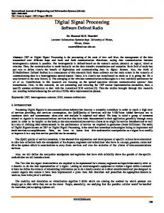
Convolution: A visual Digital Signal Processing (DSP) tutorial R.C. Kim (02-21-2014; updated 01-02-2015)

Introduction: Fourier theory says that any periodic signal can be created by adding together different sinusoids (of varying frequency, amplitude and phase). In many applications, an unknown analog signal is sampled with an A/D converter and a Fast Fourier Transform (FFT) is performed on the sampled data to determine the underlying sinusoids. In this 7-step tutorial, a visual approach based on convolution is used to explain basic Digital Signal Processing (DSP) up to the Discrete Fourier Transform (DFT). The DFT is explained instead of the more commonly used FFT because the DFT is much easier to understand. (The DFT is equivalent to the FFT except the DFT is far less computationally efficient.) In particular, convolution is shown to be the key to understanding basic DSP. Also, some of the concepts are far more intuitive in the frequency-domain vs. the more familiar time-domain. Note: The distinction between continuous and discrete systems is blurred in this tutorial since the concepts are similar for both. Most of the following figures show continuous signals (except where as noted) for clarity because sampled signals are literally discrete (i.e. “dots”) and have the added complication of spectral replicas as will be explained in Step 6. Step 1: Convolution review Any linear system’s output, y(t), can be determined by the equation: y(t) = h(t)* x(t) where x(t) is the input; h(t) is the system’s impulse response and “*” represents convolution. A system’s response to an impulse input tells us the complete frequency response of that system. It does so because an impulse, which is a mathematical abstraction, consists of an infinite number of sinusoids of all frequencies, i.e. it excites a system equally at all frequencies. An ideal impulse is infinite at t=0 and 0 elsewhere in the time-domain (Figure 1(a)). 1(b-c) shows an ideal impulse is approximated by adding up an increasing number of sinusoids. (The sinusoids add up to create an infinite spike at t=0 and cancel to 0 everywhere else.) Figure 1(d) shows the ideal impulse in the frequency-domain (it’s a flat, infinite horizontal line since all frequencies are equally represented with the same magnitude). 1(a) and 1(d) are an example of duality between the time and frequency domains: narrow signals in one domain are wide in the other domain.

FIGURE-1: Impulse Function: (a) Ideal impulse in time-domain; (b) Sum of 10 sinusoids; (c) Sum of 75 sinusoids; (d) Ideal impulse in frequency-domain

Convolution: A visual DSP Tutorial

PAGE 1 OF 15

dspGuru.com

For discrete systems, an impulse is 1 (not infinite) at n=0 where n is the sample number, and the discrete convolution equation is y[n]= h[n]*x[n]. The key idea of discrete convolution is that any digital input, x[n], can be broken up into a series of scaled impulses. For discrete linear systems, the output, y[n], therefore consists of the sum of scaled and shifted impulse responses, i.e. convolution of x[n] with h[n]. Figure 2(a-f) is an example of discrete convolution. (Don’t worry if you don’t understand it yet- it should be clearer after Step 4.)

FIGURE-2: Discrete Convolution example: (a) x[n] input; (b) h[n] impulse response (c-e) shifted impulse responses; (f) y[n] =sum of c-e

It can be proven (but it won’t here) that convolution in the time-domain is equivalent to multiplication in the frequency-domain and vice-versa: x[n] * h [n] X[f]· H[f]1. Likewise, convolution in the frequency-domain is equivalent to multiplication in the time-domain and vice-versa: x[n] · h[n] X[f] * H[f].

Step 2: Sinusoids Sinusoids are important because any periodic signal can be written as the sum of sinusoids. If you understand how DSP works with sinusoids, then you can easily extend that understanding to any linear signal.

1 X[f] and H[f] are the frequency-domain versions of x[n] and h[n].

Convolution: A visual DSP Tutorial

PAGE 2 OF 15

dspGuru.com

We start by looking at the Sine and Cosine functions in the familiar time-domain (Figure 3(a)). They’re the same except that Cosine is +90◦ (+π/2 radians) ahead of Sine.

FIGURE-3: Cosine (green) vs. +Sine (red) @ 1 MHz: (a) time-domain; (b) frequency-domain

Sine is an odd function because it’s not symmetric at t=0 (sin t = -sin (-t)). Cosine is an even function since it’s symmetric at t=0 (cos t= cos (-t)). Cosine is non-zero at 0- this means that any DC value (constant offset) in a signal is due solely to its cosine component(s) since sine is 0. Now look at Figure 3(b), which shows the frequency-domain representation of sine and cosine. The derivation of these Fourier transforms (FT) won’t be shown- however, it’s still possible to develop an intuitive feel for the frequency-domain representation.

Convolution: A visual DSP Tutorial

PAGE 3 OF 15

dspGuru.com

A sinusoid consists of one frequency, so it should be a single line in the frequency-domain. Two lines are shown (one positive and one negative) because two directions are possible. We saw that cosine is an even function in the time-domain and the same symmetry is seen in the frequency-domain. Sine is an odd function and the asymmetry is also seen in the frequency-domain, i.e. sin f = -sin (-f). In the time-domain, cosine is 90◦ ahead and we see the 90◦ phase difference in the frequency-domain as well. Negative frequency will become clearer in Step 3. Step 3: Complex numbers Now we introduce the famous Euler equation: e±jωt = cos ωt ± jsin ωt where ω= 2πf. By rearranging terms, the following equations also shown in Figure 3(b) can be derived: Cos ωt= ½ · (e-jωt + ejωt) Sin ωt= ½ · (e-(jωt-π/2) + e(jωt -π/2)) = ½ · (e-jωt · e+π/2 + ejωt · e-π/2) = ½ · (je-jωt - jejωt) Again, the full derivations won’t be shown here- however, using these equations is actually straightforward. First of all, j simply represents a +90◦ phase-shift (rotation) without any change in frequency or magnitude. (j= √-1, so if multiplication by -1 causes 180◦ rotation, then half of that is +90◦.) A more formal definition is to expand the Euler equation to include a phase offset ф: ej(ωt+ ф)= cos(ωt + ф) + jsin(ωt+ф). If ω=0 and ф= π/2 (90◦), then ejπ/2= cos π/2 + jsin π/2= 0 + j(1)= +j. In Figure 4, Sine has been rotated by 90◦, and is plotted next to cosine. The 3-d sum is a rotating spiral in the time-domain. If Sine is positive, the spiral rotates in the counter clockwise (CCW) direction. If Sine is negative, the spiral rotates in the clockwise (CW) direction (that’s all there is to negative frequency.) The speed of rotation (number of complete circles per second) is simply the frequency.

FIGURE-4: Complex-number in the time-domain

Convolution: A visual DSP Tutorial

PAGE 4 OF 15

dspGuru.com

In Figure 5(a-c), we look at the frequency-domain version of a complex number. If we rotate Sine by +90◦, then it looks like 5(b). If we then add cos A + jsin A, one of the lines cancels out, and we’re left with a single side-band (SSB) vector shown in 5(c). This single vector is static, i.e. it does not rotate or move at all.

Figure-5: Complex number in the frequency-domain (MHz): (a) cos A and sin A; (b-c) cos A + jsin A

Note: For cos A - j·sin A, the SSB vector would be at f= –A. Convolution: A visual DSP Tutorial

PAGE 5 OF 15

dspGuru.com

Figure-6: Polar form

Figure 6 shows the polar form, which is obtained from a side-view of either Figure 4 or 5(c). For the polar form, it’s common to use the notation: R< ф where R= √(I2+Q2) and ф= phase. I is the real (in-phase) component and Q is the imaginary (quadrature-phase) component as shown in Figure 62. In the time-domain, the polar form is like a rotating clock hand (ф= ωt + a phase-constant). In the frequency-domain, the polar form is like a broken clock- the clock hand does not move (ф= a phase-constant).

Step 4: Convolution with Sinusoids Most of the time, convolution is thought of only in terms of a system’s output as shown in Step 1. However, it’s actually a mathematical operation in its own right as shown next. Convolution is complicated and requires calculus when both operands are continuous waveforms. But when one of the operands is an impulse (delta) function, then it can be easily done by inspection. The rules of discrete convolution are (not necessarily performed in this order): 1) Shift either signal by the other (convolution is commutative). 2)

Multiply the magnitudes (and add any overlapping lines).

3) Add the phases.

2 I/Q are always perpendicular to each other regardless of ф. For a single complex number, any phase-offset can be set to 0 since the axis-

orientation is arbitrary. Phase really only matters when plotting multiple complex numbers, which can have any phase-offset with respect to each other. Note: I/Q have the form: i[n]+jq[n] in the time-domain; and I[f]+jQ[f] in the frequency-domain.

Convolution: A visual DSP Tutorial

PAGE 6 OF 15

dspGuru.com

Cosine-Cosine example: A simple example is the well-known trig identity: cos A · cos B= ½·cos (A+B) + ½·cos (A-B). Figure 7(a-c) shows the equivalent operation in the frequency-domain. As explained in Step 1, multiplication in the timedomain is convolution in the frequency-domain. Convolution is performed by “lifting” the function in 7(a), which is centered at f=0, and shifting the center to both f=-2 and f=+2 (7(b)). After multiplying the magnitudes (1/2· 1/2=1/4), the result in 7(c) agrees with the trig identity. In this case, the phases are both 0 so rule #3 is N/A. Figure 7(d-f) shows the case when A=B. The two “overlapping” lines at f=0 add up to create a DC value (1/4 +1/4= ½).

FIGURE-7: Cosine-Cosine convolution in the frequency-domain (real-axis only): (a-c) for different f; (d-f) for the same f

J-example: The 3rd rule of convolution is that phases add. Multiplying by j in the time-domain is convolution in the frequency-domain. Since j’s magnitude is 1 and f=0, the only effect is rotation by +90◦ (or -90◦ with –j) without any frequency-shift. Figure 8(a) show a complex number at f=1 (1