Cooperation in Multi-Agent Systems Using Learning Automata

Cooperation in Multi-Agent Systems Using Learning Automata M. R. Khojasteh

M. R. Meybodi

Soft Computing Laboratory Computer Engineering Department & Information Technology Amirkabir University of Technology Tehran, Iran Email: (mrkhojas, meybodi)@ce.aku.ac.ir

Abstract Agents are software entities that act continuously and autonomously in a special environment. It is very essential for the agents to have the ability to learn how to act in the special environment for which they are designed to act in, to show reflexes to their environment actions, to choose their way and pursue it autonomously, and to be able to adapt and learn. In multi-agent systems, many intelligent agents that can interact with each other, cooperate to achieve a set of goals. Because of the inherent complexity that exists in dynamic and changeable multiagent environments, there is always a need to machine learning in such environments. As a model for learning, learning automata act in a stochastic environment and are able to update their action probabilities considering the inputs from their environment, so optimizing their functionality as a result. Learning automata are abstract models that can perform some numbers of actions. Each selected action is evaluated by a stochastic environment and a response is given back to the automata. Learning automata use this response to choose its next action. In this paper, the goal is to investigate and evaluate the application of learning automata to cooperation in multi-agent systems, using soccer server simulation as a test-bed. Because of the large state space of a complex multi-agent domains, it is vital to have a method for environmental states’ generalization. An appropriate selection of such a method can have a great role in determining agent states and actions. In this paper we have also introduced and designed a new technique called “The best corner in state square” for generalizing the vast number of states in the environment to a few number of states by building a virtual grid in agent’s domain environment. The efficiency of this technique in state space generalization in a cooperative multi-agent domain is investigated.

Keywords: Learning automata, Agent, Multi-agent systems, Simulated robotic soccer, Team of agents, Cooperation 1

- INTRODUCTION

Multi-agent systems have formed a good research area recently with wide industrial and commercial applications. An agent is an autonomous entity that has some characteristics including being social, reflective and proactive. Agents live in an environment that can be open or closed. This environment can have some other agents in itself either. Agents cooperate with each other in order to achieve better individual or social goals. When a group of agents in a multi-agent system share a long-term goal, they form a team. In fact, a group of agents make a cooperative team when: • All agents have a common goal. • Each agent plays its role in order to achieve that common goal.

•

[1].

Each agent responds to a query for taking its role

Members of a team (or teammates) coordinate their behaviors with each other based on adapting their cognitive processes with each other and based on the direct effects on each other’s inputs through communication activities. Because of the large state space that a complex multiagent domain may have, it is vital to have a method for environmental states’ generalization. An appropriate selection of such a method can have a great role in determining agent’s states and actions. In the first part of this paper we have introduced and designed a new technique called “The best corner in state square” for mapping the vast number of continuous states in the environment to a few

number of discrete states by building a virtual grid in the agent’s domain environment. As a model for learning, learning automata act in a stochastic environment and are able to update their action probabilities considering the inputs from their environment, so optimizing their functionality as a result. In the second part of this paper, the efficiency of learning automata for cooperation between agents in a team has been investigated. As a test-bed we used the simulated robotic soccer, “SoccerServer”. Robotic soccer is an example of a complex environment that some agents should cooperate with each other, in order to achieve the team’s goal [3][4][5][6]. In fact, in this paper we have focused on the systems composed of some autonomous agents that can act in real-time, noisy,

collaborative and adversarial environments [2]. To do so, we implemented teams composed of 2, 5, and 11 agents that learn using learning automata and compared them to similar teams that has no learning capability or using other learning methods such as Q-learning. In the coming sections of this paper, we first investigate the learning automata as a method of learning and then we introduce the technique “The best corner in state square” as a method for generalizing environmental states and at last, the result of simulations are presented. 2

- LEARNING AUTOMATA

Learning automata (LA) can be classified into two main families, fixed and variable structure learning automata

[7][8]. Examples of the fixed structure type are Tsetline,

variable-structure automata. We summarize some of fixedstructure learning automaton and variable structure automaton in the following paragraphs. The two-state automata (L ) : This automata has two states, φ and φ and two actions α and α . The automaton accepts 2,2

1

2

• • •

•

α = {α1, ... , αr} is the set of actions that it must choose from. Φ = {φ1, . . . , φs} is the set of internal states. β={0,1} is the set of inputs where 1 represents a penalty and 0 represents a reward. F: Φ β Φ is a map called the state transition map. It defines the transition of the state of the automaton on receiving an input, F may be stochastic. G : Φ→ α is the output map and determines the action taken by the automaton if it is in state φj.

2

response). An automaton that uses this strategy is refereed as L where the first subscript refers to the number of states and second subscript to the number of actions. The two-action automata with memory (L ): This 2 ,2

2N,2

automaton has 2N states and two actions and attempts to

incorporate the past behavior of the system in its decision rule for choosing the sequence of actions. While the automaton L switches from one action to another on receiving a failure response from environment, L keeps an account of the number of success and failures received for each action. It is only when the number of failures exceeds the number of successes, or some maximum value N; the automaton switches from one action to the another. The procedure described above is one convenient method of keeping track of performance of the actions α and α . As such, N is called memory depth associated with each action, 2,2

2N,2

1

2

and automaton is said to have a total memory of 2N. For

every favorable response, the state of automaton moves deeper into the memory of corresponding action, and for an unfavorable response, moves out of it. This automaton can be extended to multiple action automata. The state transition graph of L automaton is shown in figure 1. 2 N,2

Krinsky, TsetlineG, and Krylov automata. A fixed structure learning automaton is represented by a quintuple 〈α , Φ, β , F, G〉 where: •

1

input from a set of {0, 1} and switches its states upon encountering an input 1 (unfavorable response) and remains in the same state on receiving an input 0 (favorable

1

2

N- 1

N

2N

N+ 2

N+ 1

N+ 2

N+ 1

F av o r a b l e Re s p o n s e ( β = 0 )

1

2

N- 1

N

2N

Un f a v o r a b l e Res p o n s e ( β = 1 )





Figure 1: The state transition graph for L

2N,2

The Krinsky automata: This automaton behaves exactly like L automaton when the response of the environment is unfavorable, but for favorable response, any state φi (for i = 1, . . . N) passes to the state φ and any state φi (for i = N+1, 2N) passes to the state φ . This implies that a string of N consecutive unfavorable responses are needed to change from one action to another. The state transition graph of Krinsky automaton is shown in figure 2. 2 N,2

1

N+1

The selected action serves as the input to the environment, which in turn emits a stochastic response β(n) at the time n. β(n) is an element of β={0, 1} and is the feedback response of the environment to the automaton. The environment penalize (i.e., β(n) = 1) the automaton with the penalty ci, which is the action dependent. On the basis of the response β(n), the state of automaton is updated and a new action chosen at the time (n+1). Note that the {ci} are unknown initially and it is desired that as a result of interaction with the environment the automaton arrives at the action which presents it with the minimum penalty response in an expected sense. If the probability of the transition from one state to another state and probabilities of correspondence of action and state are fixed, the automaton is said fixedstructure automata and otherwise the automaton is said

N

1

2N

N+ 1

Fav or ab le Re spo nse ( β = 0)

N

1

2N

N+1

Unf avo r ab le Re spo nse ( β = 1)

Figure 2: The state transition graph for Krinsky Automaton The Krylov automaton: This automaton has state transition that is identical to the L automaton when the output of the 2N,2

environment is favorable. However, when the response of the environment is unfavorable, a state φi (i ≠1, N, N+1, 2N) passes to state φ with probability 0.5 and to state φi- with probability 0.5. When i∈{1,N+1}, φi stays in the same state with probability 0.5 and moves to state φ with the same probability. When i = N, automaton state moves to state φNand φ with the same probability 0.5. When i = 2N, automaton state moves to state φ - and φN with the same probability 0.5. The state transition graph of this automaton i+1

1

i+1

1

2N

2N 1

is shown in figure 3.

N

1

/

/

1 2

2N

F a v o r a b l e R e s p o n s e (β = 0)

1 2

N+1

/

/

1 2

N

1

2N

1 2

N+1

U n f a v o r a b l e R e s p o n s e (β = 1)

Figure 3: The state transition graph for Krylov Automaton Variable Structure Automata: Variable-structure automaton is represented by sextuple 〈α, β, Φ , P, G, T〉, where β a set of inputs, Φ is a set of internal states, α a set of outputs, P denotes the state probability vector governing the choice of the state at each stage k, G is the output mapping, and T is learning algorithm. The learning algorithm is a recurrence relation and is used to modify the state probability vector. It is evident that the crucial factor affecting the performance of the variable structure learning automata, is learning algorithm for updating the action probabilities. Various

amount of increase (decreases) of the action probabilities. For more information on learning automata the reader may

refer to [7..11].

- THE “THE BEST CORNER IN STATE SQUARE” TECHNIQUE 3

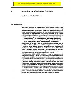
The number of states in a simulated robotic soccer domain is very large and therefore, for an agent to consider all of them is impossible. In fact, the most important job in this regard, is to design a proper generalization of the environmental state space for the agent. If we call the set of agent’s actions A, each agent will have |A| possible actions in each of |V| states and therefore, the set to be learned for the agent will have at most V × A elements. If we choose the sets V and A wisely, our agents can learn effectively in a complex and real-time environment using limited samples. In fact, the sets V and A should have the property that cover all states and actions as much as possible and they should be good mappings of the sets of all possible states and actions that exist in the domain of agents. For generalization of the environment, we divide the

field of soccer into 150 equal squares each with side length 7.

By doing so, at any moment of the simulation, each agent is in one of these squares. Considering the fact that each agent has a limited view of its environment, it can’t count on the whole

field. So, we have focused on 24 squares around the square that has the agent in it as shown in figure 4:

learning algorithms have been reported in the literature[7][8]. Let αi be the action chosen at time k as a sample realization from distribution p(k). The linear reward-inaction scheme the recurrence equation for updating p is defined as

p j(k ) =

      

p j(k ) + a  1 - p j(k )

if i = j

p j(k )(1 − a)

if i ≠ j

(1) Figure 4- 24 squares around the square X which has the agent

if β is zero and P is unchanged if β is one. The parameter, a which is called step length, determines the amount of increases (decreases) of the action probabilities. In linear reward-penalty algorithm (LR-P) scheme the recurrence equation for updating p is defined as

p j(k ) =

      

p j(k ) + a  1 - p j(k )

if i = j

p j(k )(1 − a)

if i ≠ j

if β(k) = 0

(2)

and

 p j(k) 1 - b  p j(k ) =   b + (1- b) p j(k)    r -1

(

)

if i = j if i ≠ j

(3)

if β(k) = 1. The parameters a and b represent reward and penalty parameters, respectively. The parameter a(b) determines the

In figure 4, the squares X+10, X+11, X+1, X-9, X-10, X11, X-1, and X+9 are called the immediate squares for the square X. Note that we have assigned numbers to each square from left to right of the field and also vertically, by starting from 0 for the first square located in the upper left and ending

in 149 for the last square located in the extreme lower right. So, we have 10 squares in each column and 15 squares in each row. We have considered a numeral quantity for each of these 8 squares (directions) around the agent; the north-west square, the north square, the north-east square, the east square, the south-east square, the south square, the south-west square, and the west square. In the following figures, we have shown the squares in the 8 directions around the agent as we mean in this paper. Note that we have used north for the direction toward the opponent’s goal.

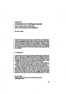
(relative to itself) these teammates and opponents are located in. In fact, the agent that possesses the ball, calculates “the best corner in state square” that is its state, by finding the

maximum value of the quantities for each of its square’s 8

corners gained by the above-mentioned process. In order to

have a good feeling for the 24 squares around each agent that

collectively form the “local” or “important” space for it, let’s

Figure 5- North-west, north-east, south-west, and south-east squares around the square that has the agent and the 4 main directions shown.

have a look at figure 7. In this figure, the local and important

space for an agent that uses “the best corner in state square” technique is shown in white color. The agent uses only this space to determine the proper decision. This figure shows a

play of 4 against 4. In this figure, the teammate number 2 and the opponents 1 and 2 are of importance to the agent that

possesses the ball because they are in agent’s local space. Because the current state for each agent in the environment at time t, depends heavily on the distance and the angle of other agents relative to it, we have also used these state squares for determining different formations for the team and for the positioning of each player on the field.

Figure 6- North, east, west, and south squares around the square that has the agent and the 4 main directions shown. If the agent located in square X sees one of its opponent agents in one of its north-west squares (squares X+9, X+8,

X+18, and X+19), it adds a negative quantity to its

corresponding direction (in this case north-west) quantity. This would be vice versa in the case that the agent sees a teammate. As an example, if the agent that has the ball in its possession (located in square X) sees one of its teammates in any of the squares that we have considered as south-west squares (squares X-21, X-22, X-11, and X-12), it adds a positive quantity to its corresponding direction (in this case south-west) quantity. The quantity added to the direction quantities is conversely proportional to the distance of the mentioned agent (opponent or teammate) in that direction from the agent that has the ball. In fact the agents that are

closer to the agent that has the ball (and are located in the 24 squares around its square) have more effect on its direction quantities than the agents that are far (and of course still located in the above-mentioned 24 squares) from it. Note that we haven’t considered any effects on the agent’s direction

quantities for the agents that are outside the above 24 squares. As a result, by computing the overall positions of the

agents (opponents or teammates) that are located in the 24 squares around its square, each agent will have 8 numbers. By assigning these 8 numbers to the 8 directions around the agent and choosing the maximum of these quantity at any instant, we will have 8 states and 8 actions. Each action corresponds to sending the ball to the center of one of its immediate squares for the agent that possesses the ball. By doing so, we have reduced the state space around the agent to 8 states that seem to cover all the states in that space. The similar states are mapped into a unique state. It is obvious that in any time instant t, there may be any number of

teammates and agents in the 24 squares around the agent’s

square. If any of these agents are located in the same square that the mentioned agent is located in, the agent will change

its numeral quantities depending on which of the 8 directions

Figure 7- The status of teammates and opponents regarding the local space of the agent that possesses the ball

(in a play of 4 against 4)

Note that selecting a state (or corner) by the agent that possesses the ball in the above case doesn’t mean that this agent should send the ball to the center of the immediate square (or toward the corner) that is associated with that state.

This state just shows one of the 8 states that the ball possessor

can be in it. It is clear that in each state, the agent can choose

one of its 8 possible actions (sending the ball to the center of

each of its immediate squares) independently of the state selected. Although our definition of the state for the possessor of the ball may lead us think that the direction for sending the ball should be to the center of the immediate square corresponding to the selected (corner or) state, but in a lot of cases, this won’t be the optimum action for our agent. So, our states are independent of the best possible action that can be

done in them. Therefore, each agent has at most 64 elements to be learned (8 possible actions in each of 8 possible states). In

fact, in each state, each agent chooses its optimal action (in that state) using the corresponding learning automata. The overall scenario for each agent in our simulations is like this: if the possessor of the ball sees any player in its way toward the opponent’s goal, it determines its state and then use the corresponding learning automata (for that state) to select its optimal action that seems to be effective in order to achieve the common goal of the team. Also, if any player sees a teammate possessing the ball, tells it its own position

and also the positions of the players that it sees to help it for a better estimate of the state that it is in and consequently, to help it to have a better action. Note that every agent has a limited view of the field and so it doesn’t see its sides and its back and so it is vital to use the hearing (or the communication) facility in these cases as mentioned above. This is our only (limited) use of hearing in our simulations. In fact, in these situations, the player without ball tells its world model to the teammate that has the ball to help it to choose its right action. Also, the player without the ball, goes to the center of the immediate square that finds it proper for receiving the ball from its teammate that has the ball. Therefore in our simulations, the player without the ball can have its own states and its own actions for moving to one of

the 8 directions in order to receive the ball.

Also in our method, the player is not forced to move (pass or shoot) forward in all states and it may (as the result of one of its 8 actions) passes back, dribbles, sends ball to out, or shoots the ball to an empty space in the field if it finds it more appropriate in if it is probable that a teammate or itself in some cycles later chases the ball in that satae. It is necessary to note that our agents’ learning in all of our simulations is fully multi-agent and distributed and is not like the methods used in the litrature that the player with the ball tells its intent to whom it may sends the ball. So, each agent is completely autonomous in choosing its action and tries to learn cooperation with its teammates with a little use of communication

- COOPERATION IN A TEAM USING LEARNING AUTOMATA 4

Our goal in this section is to use learning automata for cooperation among the members of a team in order to achieve a common team goal. In the simulations conducted, we have tested plays between some players that learn using learning automata and some players that learn using the other methods of learning or some players that don’t have learning capability. Note that the “without learning” teams in our simulations are like the “learning” teams from every aspect (architecture, states, actions, etc.), except that they can’t learn from their previous experiences. By now, various machine learning methods such as Q-learning, genetic algorithms,

decision trees, behavioral learning[2], to mention a few, have

been used for training the soccer player agents. To our knowledge, this resaearch is the first attampt to use learning automata in cooperation in multiagent systems.

4-1- SIMULATIONS FOR TEAMS WITH 2 PLAYERS In the first series of simulations , there are two players in each team. These series of simulation were done with two methods for determining agent’s state in its environment: simple generalization and “the best corner in state square” technique.

In section 4-1-1 simulations for simple generalization and in section 4-1-2 simulations for “the best corner in state square” technique are reported.

4-1-1 – SIMPLE GENERALIZATION In the simple generalization method we map the state of the

player with the ball into 4 states and the state of the player without the ball also into 4 states. For each of these 4 states,

we use a fixed structure learning automata with memory depth

3. Each automaton, has two actions. For example for the player

that posseses the ball, these two actions are defined to be passing the ball to the other teammate or shooting toward the opponent’s goal. The first results obtained showed that the team using learning automata when plays against the team

without learning, easily defeats its opponent. We conducted 50 plays between the teams using fixed structure learning

automata versus the “without learning” team, and 50 plays

between the team using Q-learning versus the “without

learning” team. The average goals scored in 50 plays between are given in table 1. In this table, the right number shows the number of goals scored by the learning team and the left number shows the number of goals received by the learning team. As the results show, all the plays have been finished with the victory of the learning teams. It is necessary to point out that in the above table, column 1 is the cumulative result of the plays from cycle

0 till cycle 999, column 2 is the cumulative result of the plays from cycle 1000 till cycle 1999, …, and at last column 6 is the cumulative result of the plays from cycle 5000 till cycle 5999

(the end of a standard play in soccerserver simulator). As the table shows, there isn’t a notable difference in performance for teams using L 2 n , 2 , G 2n , 2 , and Krylov automata. But teams

using Q-learning[2] and the results.

Krinsky automata showed better

REMARK 1: Simulation results show that the learning automata team learns to pass and shoot more accurately as more games played. Because of this, most of the goals received by the learning team is in the first half of the game (first 3000 cycles). The learning team controls the play in the

second half of the game and scores most of its goals (second 3000 cycles). Other series of simulations showed us that teams

equipped with learning automata (with 2 players) defeated the “without learning” teams even with more players (3 or 4 players).

REMARK 2: In simulations we observed that our multi-agent learning method is to some extent dependent on the opponent behavior. In fact, there is not a predetermined convereged values for our players’ memory values. Our simulations, in most cases, reject our predictions for memory values. This means that our players may learn to shoot to opponent’s goal in in cases that its more appropriate to pass. Table 1- Average goals scored in 50 plays between learning teams with 2 players versus the “without learning” team with 2 players 6 5 4 3 2 1 5-16 5-12 4-9 4-7 3-3 2-1 L 2n , 2

5-16 3-13 2-10 2-8 1-5 1-2

G 2n , 2

4-17 3-15 3-11 3-7 2-4 1-2

Krinsky

3-12 3-11

Krylov

3-9

2-6 1-4 1-2

4-17 3-15 3-13 2-10 2-5 1-3

Q

4-1-2- “THE BEST CORNER IN STATE SQUARE” One of the problems with the previous simulations was the possibility of mapping a lot of various states to a single state and so, it was possible that the action selected by the agent as the best action to be performed in that state, would not be the best choice. Another problem with previous simulations was the few number of possible actions defined for each agent; “passing to the teammate” and “shooting to the opponent’s goal” Therefore, we used the technique “the best corner in state square” in order to have a better

generalization of the environment states. We also used 8

automata for each agent (one automaton for each corner that

1.17 1.25 1.30 0.82 1.18 1.05 1.07

shows the present state of the agent) and 8 actions for each agent , sending the ball to the center of one of agent 8

1.12

immediate squares as defined in the “The best corner in state square technique”.

1.02

We conducted some simulations between a team which uses the technique “the best corner in state square” and a team which uses the generalization technique of previous section. Both teams were made of 2 players. Totally 30 plays were simulated. In these plays, the L rp team won 28 times and just one of the plays was won by the apponenet

[13].

We repeated the previous simulations using “the best corner in state square” technique with different kinds of learning automata (fixed and variable structure) and for Q-

learning. The results showed [13] that by using “the best

corner in state square” technique, the agent performs better in determining its own state and consequently, in determining the proper action in that state. We also did another simulation between two teams which we call them “complete (squares) learning” and “fixed mapping”. For team “complete (squares) learning”, we put 8 automata in each square of the agent’s grid-like environment. By doing so, the agent did not carry its automaton with itself as it moved from one squre to another. Team “fixed mapping” is a team with hand-optimized code. These two teams play against each other. The ratio of the number of goals scored versus the number of goals received by the learning team when playing versus the “without learning” team for different learning automata is given in table 2. The results obtained confirm that the technique “the best corner in state square”, does a proper generalization for

automata with memory depth 2 (10 plays) G 2n , 2 automata with memory depth 3 (10 plays) Krylov automata with memory depth 3 (10 plays) Krinsky automata with memory depth 3 (10 plays) L rp automata (30 plays) L ri automata (15 plays) L r ε p automata with parameter ration 0.1 (30 plays) L rεp automata with parameter ration 0.01 (30 plays) Q-learning (10 plays) L 2 n, 2

4-2- SIMULATIONS FOR TEAMS WITH 5 PLAYERS In this section, we present the results of a set of simulations

for teams with 5 players as used in “Middle Size Robocup

branch” and “Indoor Soccer”. The main difference between this set of simulations with the simulations presented in the previous section is that, in the these simulations we have considered formation for each team in the play, that is giving an special place to each player in the field. This seems to be necessary because as the number of players in the team increases, a team formation is needed for a better cooperation among the teammates. In these series of simulation, we implemented the teams L 2 n , 2 (as a fixed structure learning automata team), L rp (as a variable structure learning automata team), Q-learning (as a team that uses another method of learning), and a “complete

learning” team [13]. In these simulations, each team has one goalkeeper, two pistons, one back defender, and one forward ,and an special area in the field is assigned to each of the above-mentioned players (or roles). These areas are in fact, a set of squares defined in the technique “the best corner in state square”. Each of the above learning teams play against the “without learning” team. The following figures show the number of goals scored and received by the learning teams which shows the effectiveness of learning automata as a learning method in such a complex domain.

the environment states[13].

scored goals by the learning teams

Table 2- The ratio of the scored goals to the received ones in various

L2n,2

learning methods using the technique “the best corner in state

70

square” in plays with 2 player teams (during training)

Lrp

60 50

The ratio of the goals scored versus the goals received During training

1.26

Method’s name

scored goals

QL

40

complete learning

30 20

complete learning from zero

10 0

1

learning teams

L 2n , 2 automata with memory depth 3

(10 plays)

Figure 8- The goals scored by the learning teams with 5 players in 10 simulations (during training)

received goals by the learning teams

Lrp Lrep Lri Krinsky Krylov

6 L2n,2

7

5

6

Lrp

4

5

received goals

QL

4

3

3

G2n,2

2

2

complete learning from zero

1 0

L2n,2

complete learning

1

0

learning teams

Figure 9- The goals received by the learning teams with 5 players in 10 simulations (during training)

4-3- SIMULATIONS FOR TEAMS WITH 11 PLAYERS In this part of the paper we investigate the case where

there are 11 players in each team.

Full_Lrep QL without learnin

1

In this series of

simulations in addition to the number of goals scored and received, the following citeria are used to measure the degree of cooperation among the team members. • The percentage of possession of the ball for each team during the simulation. • The percentage of ball movement in each 1/3 of the field. • The maximum duration time (in cycles) that each team has the ball in possession during the simulation. • The maximum number of passes between the members of each team (without being cut by members of the oponenets team) during the simulation. • The percentage of “right actions” versus the “wrong actions” done by each player of the team during the simulation. Also in these simulations we used 4-3-3 formation for each team for organizing the eleven players in the field. We implemented the teams L 2n , 2 (as a fixed structure learning

Figure 10- The ratio of the average goals scored to the average goals received for each team, during the first 15 training plays 8

Lrp

7

Lrep

6

Lri Krinsky Krylov

5 4

L2n,2

3

G2n,2

2

Full_Lrep QL

1 0

Figure 11- The ratio of the average goals scored to the average goals received for each learning team for 3 testing plays (after training plays)

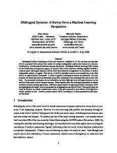
These figures show that the variable structure learning automata teams have a better performance in defeating the “without learning” team. This means that variable structure learning automata teams exhibits higher ability of learning. Another series of simulations were conducted using “fixed mapping” team (that was optimized by hand) as an oponenet. The following figure shows the number of goals scored and received by the learning teams.

automata team), L rp (as a variable structure learning automata team), Q-learning (as a team that uses another

method of learning), and a “complete learning” team [13].

Each of the above learning teams play against the “without learning” team. Note that “without learning” team is like the learning teams even in team formation except that it lacks the learning ability. The simulation results show that the learning automata teams could defeat the “without learning” team after a few number of training plays. Figures 10 and 11, show the result

of the simulations. The number of training plays is 15 and the number of testing plays is 3.

Figure 12- The received goals (the front bars) versus the scored goals (the rear bars) for different teams when playing against the “fixed mapping” team ( from left to right: “without learning”, Q-learning, “Complete learning” of L r εp , L rp , L ri , L r ε p , L 2 n , 2 , Krylov, Krinsky, and G 2 n , 2

– EVALUATION TESTS FOR TEAMS USING LEARNING AUTOMATA

5

[12][13][14][15]. In this section we evaluate our learning

method by holding simulation plays with some of the teams that had recently taken part in the world RoboCup competitions. Also we investigat the efficiency of learning automata in our agents by changing soccerserver parameters and observing their effects on the performance . It is necessary to note that our base code is the code of

goals

In the previous sections, we investigated the efficiency of using learning automata in doing a teamwork

50 45 40 35 30 25 20 15 10 5 0 1

2

3

4

5

6

7

8

9

10

plays

CMUnited98 team [2].

received

scored

In doing so, we used the following teams that were somewhat similar to our team from the individual behaviors’ point of view (although they were better) to play with

Figure 13- the number of goals scored versus the number of goals received by the learning team during 10 consecutive training plays

similar team to our team (again from the individual behaviors’ point of view) and therefor was the best choice for evaluating our team. We let our learning automata teams play against this team and observed the results in detail [13]. The results of plays with the other teams mentioned above are also reported later in this paper. In this section, we use the teams “complete learning team

In the second series of simulations, we studied the effects of single-channel, crowded, and unreliable communication provided by soccerserver on the performance of the proposed learning method. It should be indicated that because of our emphasis on the autonomy of the agents we used the least possible use of inter-communication between the agents during the simulation. The use of the communication facility is just a little, comparing to the other known teams. We

Arvand 2000, Cyberoos 2000, FuzzyFoo 2001, and Saloo 2001. Among these team, Saloo 2001 [16] was the most

of L r ε p

”

and also “L r ε p learning automata” (both based on

L r ε p automata) for our simulations. Selecting these automata are because of the good results obtained for them in the privious simulations. For more simulations the reader may

refer to [12][13][14][15].

In this section, we investigate the performance of our learning method in the environmental situations which are more difficult for the agents to adapt to than the situations we have considered so far. There are several parameters in the

when played versus the team “without learning”, as the noise increases

simulated 10 consecutive plays between team L r ε p (learning from zero) and the “without learning” team. Figure 14 shows the efficiency of our learning method and indicates that by playing more games, the learning team, adapts to the situation better and increases its gap with the “without learning” team.

simulations conducted, we study the effect of the “rand” parameters. (that indicate the amount noise values) in the soccerserver. We changed the parameter “player_rand” from

0.1 to 0.2, the parameter “ball_rand” from 0.05 to 0.1, and at last the parameter “kick_rand” from 0.0 to 0.1. The first

parameter mentioned enables us to add noise to the players’ movements and the second and the third parameters, add noise to the ball movement and kicking the ball. In this section, we also breifly discuss the speed of convergence of our learning automata algorithms used by the agents and also suggeste some techniques for increasing the speed of convergence. At the end of this section, we have investigated the effects of different formations on the teamwork. In the first series of simulations ten consecutive plays between team L r ε p (learning from zero) and the “without learning” team were simulated. Our goal was to investigate the efficiency of our learning methods and see how our team perform against “without learning” team in the presence of

noise. Figure 13 shows the cumulative results of this

exprimentation. As the figure shows, by playing more games, the learning team, adapts itself to the situation more and more and increases its gap with the “without learning” team. This figure shows the efficiency of the proposed learning method when the environment is noisy.

goals

soccerserver that one can change[3]. In the first series of

35 30 25 20 15 10 5 0

1

2

3

4

5

6

7

8

9

10

plays received scored

Figure 14- the number of goals scored versus the number of goals received by the learning team during 10 consecutive training plays when played versus the team “without learning”, without the communication facility between the agents

In the third series of simulations, we eliminated 3 players from the left side of our team; player number 2 from the defense line (the left defense), player number 6 from the middle line (the left half-back), and player number 10 from the forward line (the left forward) of our team [13]. Our goal was to evaluate the function of the team in the case of failure

in the function of some of the players. We simulated 15 consecutive plays between team L r ε p (learning from zero)

and the “without learning” team (with 11 players). Figure 15 shows the results of this expriment. Since each player has a

limited freedom around its special post in the field, simulation show that this elimination causes our team’s left side to malfunction. Note that we have used the 4-3-3

formation for our teams. As figure 15 shows, our learning

team was able to overcome the absence of its players and adapt itself to fewer number of players and finally defeated the “without learning” team. In the fourth and fifth series of simulations, we investigated the efficiency of our learning method

when“wind” blowing in the field. Figures 16 and 17 show

the effect of wind on the performance of the proposed

method. As figure 16 shows the learning team had been able

Figure 17- The number of goals scored versus the number of goals received by the learning team during 10 consecutive training plays when playing versus the team “without learning”, with adding wind

vector (50,0) to the simulation field (horizontal wind toward the learning team’s goal)

REMARK 3:

In the seventh series of simulations, we

made some simulations between team L r ε p (learning from zero) and team Saloo and the results of the first seven plays are gathered in table 3. As the table shows, team Saloo could win all the first games with relatively high goal average

to overcome the wind and finally won the games. In figure

(average scored goals of 5.7 versus average received goals of 0.3 in each play), and has an absolute better performance

our team, it could finally stop the opponent.

than our team. We taught that our team may need more training plays in order to be able to defeat the team Saloo.

17, despit the fact that there was a really bad condition for

So, we simulated 150 consecutive plays (equal to 25 hours) between the two teams. During these 150 simulated plays (that the result of first 7 plays came in table 3), our team

45 40 35

could improve its performance and gradually move toward “not losing" and finally to continuously “win” . The statistics

goals

30

of the last 7 plays are given in table 4. In these plays, an average scored goals of 3.6 and an average received goals of 0.1 is obtaied. Although team Saloo performance is degrafed

25 20 15 10 5 0

1

2

3

4

5

6

7

8

9

10

11

12

13

14

15

plays

received

scored

Figure 15- The number of goals scored versus the number of goals received by the learning team during 15 consecutive training plays

when playing versus the team “without learning”, with eliminating

goals

3 players from the left side of the learning team

50 45 40 35 30 25 20 15 10 5 0

Table 3- The statistics for the first 7 plays between team L rε p

52.6

1

2

3

4

5

6

received

7

8

9

10

scored

Figure 16- The number of goals scored versus the number of goals received by the learning team during 10 consecutive training plays

when playing versus the team “without learning”, with adding wind

vector (0,50) to the simulation field (vertical wind in the field) 40

47.4

The percentage of possession of the ball for the opponent team (Saloo) The percentage of possession of the ball

10.5

for the our team (L rε p ) The percentage of ball movement in

47

The percentage of ball movement in the

42.5

The percentage of ball movement in our

435

The maximum continuous time that opponent team has the ball in possession The maximum continuous time that our team has the ball in possession The maximum number of continuous passes between the members of the opponent’s team The maximum number of continuous passes between the members of our team

112 14 8

35 30 goals

team’s players in the first 7 plays and in the last 7 plays. (learning from zero) and team Saloo

plays

25 20 15 10 5 0

as it plays more more games but it has higher grade on some of the criterias defined before. For example for “percentage of right actions versus the wrong actions ” team Soloo has an upper hand. In table 5, for the sake of comparison, we give the average percentage of wrong actions for the learning

1

2

3

4

5

6

7

plays received

scored

8

9

10

opponent’s 1/3 of the field middle 1/3 of the field 1/3 of the field

Table 4 - The statistics for the last 7 plays (after 25 hours training) rε p

between team L (learning from zero) and team Saloo

45

The percentage of possession of the ball for the opponent team (Saloo) The percentage of possession of the ball

55

42

for the our team (L rε p ) The percentage of ball movement in opponent’s 1/3 of the field The percentage of ball movement in the

33.5

The percentage of ball movement in our

112.7

The maximum continuous time that opponent team has the ball in possession The maximum continuous time that our team has the ball in possession The maximum number of continuous passes between the members of the opponent’s team The maximum number of continuous passes between the members of our team

24.5

1/3 of the field

8.8 12

Table 5 -Average wrong actions’ percentage for each agent of the team L

enough training).

Table 6- The average percentage of right actions (passes for each player for two methods: decision tree used in CMUnited98, and learning automata used in our teams

The percentage of the right actions (pass evaluation)

65% 76.4%

middle 1/3 of the field

134.2

rε p

wrong actions comparing to CMUnited98’s (of course after

in the first 7 plays and the last 7 plays (after 25 hours of training) when played versus team Saloo

Wrong actions’ percentage

40.1 24.6

In the first 7 plays In the last 7 plays

REMARK 4: It is necessary to remind that our agent tries to

send the ball toward one of its 8 directions, whichever seems to be better for achieving the team’s goal [12][13][14][15]. This action might (relative to position) be as a pass, a

dribble, a shoot, or else. In team CMUnited98, there are two

layers for multi-agent behavior (pass evaluation that is trained offline using decision trees) and for team behavior (pass selection that is trained online using a method based on Q-learning which uses the output of the previous mentioned

layer as the input) [2]. Our method for learning has combined the above two layers into one layer. We use some offline training before the team play against another team. We haven’t separated “pass evaluation” from “pass selection”. In fact we are dealing with actions that a player choose and whether or not the action choosen is right action. We aren’t involved with “pass” as a problem to solve. Instead, we have looked at the problem of “cooperation between our agents”. So to compare the efficiency of our method with that of other

methods like Stone’s method [2] in CMUnited98 we better

compare “the percentage of the right actions taken by the players” with “Stone’s percentage of CMUnited98’s players’

successful passes”. As table 6 shows, Stone method has 65% successful pass evaluation (the second layer in his layered learning [2]) whereas our method has chosen the right action 76.4 percent of the time. As this table shows, in

our method the players on average, does lesser number of

Decision tree Learning automata (L r ε p )

REMARK 5: As an end to this research, we investigated the effects of different team formations on the agents’ cooperation. Note that for all the simulation presented so far we have used 4-3-3 team formation. We created similar teams (L r ε p ) but with different formations 4-4-2, 3-6-1, 4-33, 3-5-2, and 3-4-3 and then simulated a series of plays

between them. Figure 18 shows the results of these simulations [13]. As the results show it is very important to

have a proper team formation in order to achieve a good

team performance. Figure 18 shows that the highest number of goals scored was by the team with the formation 3-5-2 and the least number of goals received was by the team with the formation 4-4-2. From the result of simulations we may conclude that it is wise to use a team formation that has had the most scored goals against a team that defends in most of the times and also, it is wise to use a team formation that has had the least scored goals against a team that attacks in most of the times. So we may add another layer, called team strategy layer, to the proposed method be responsible for changing formation during the play. This layer may help us to choose a defending formation while our team has won the game and there is little time to the end of the play and similarly, to choose an attacking formation while our team has lost the game and there is not enough time to make up. We may use a usual team formation (like 3-4-3 formation) in other times of the simulation.

35 30 25 20 15 10 5 0

received scored scored

received

Figure 18- scored and received goals by the learning automata teams (L r ε p ) for different team formations playing against each other (from left to right 4-4-2, 4-3-3, 3-6-1, 3-5-2, and 3-4-3)

For simulations in which other learning automata such as

“Estimator algorithm” [17] and “Discretized Pursuit Learning Automata” [18] are used the reader may refer

to[13]. For a discussion about the speed of convergence of the proposed method and also methods to improve the speed

of convergence the redear may again refer to [13]. 6

– CONCLUDING REMARKS

The goal of this paper was to use learning automata for successful production of a series of actions for agents that were members of a team, such that the resulting team can act well in multi-agent, adversarial, noisy, real-time, and most important collaborative environments. The methods introduced are general methods that can be implemented, applied, and used in other domains or other test-beds with minor changes. In this paper we also introduced the “the best corner in state square” technique for proper generalization of the environmental states which maps similar states into one unique state. The most important characteristic of this technique is to map a continuous state space to a discrete and finite state space by forming a virtual grid on the agent’s environment and at the same time to maintain the important roles of some aspects such as distance and angle in agent’s state. The results of our simulations, show that the “the best corner in state square” technique in which the agent’s decision is based on its local space is very effective when one wants to use local cooperation in order to achieve a global team goal in cooperative and complex multi-agent domains. At last, by implementing some evaluation tests and observing the results, the efficiency of learning automata in cooperation among a team agents which are seeking a common team goal is evaluated..

References:

1- Weiss G.,

Multi-agent Systems: A Modern Approach to Distributed Artificial Intelligence, The MIT Press, London,

1999.

2- Stone P., Layered Learning in Multi_Agent Systems, PhD thesis, School of Computer Science, Carnegie Mellon University, December 1998.

3- Noda I., Team GAMMA: Agent programming on gaea, In Kitano H., editor, RoboCup-97: Robot Soccer World Cup I, pages 500-507, Springer Verleg, Berlin, 1998. 4- RoboCup web page, 1997, At URL http://www.robocup.org. 5- Kitano H., editor, RoboCup-97: Robot Soccer World Cup I, Springer Verlag, Berlin, 1998.

6- Andre D., Corten E., Dorer K., Gugenberger P., Joldos M., Kummenje J., Navaratil P. A., Noda I., Riley P., Stone P., Takahashi R., and Yeap T., Soccer server manual, version 4.0, Technical Report RoboCup –1998-001, RoboCup, 1998. 7- Narendra K.S. and Thathachar M.A.L., Learning Automata: An Introduction, Prentice Hall, Inc., 1989. 8- Mars P., Chen J.R. and Nambir R., Learning Algorithms: Theory and Applications in Signal Processing, Control and Communications, CRC Press, Inc., pp. 5-24, 1996. 9- Lakshmivarahan S., Learning Algorithms: Theory and Applications, New York, Springer Verlag, 1981. 10- Meybodi M.R. and Lakshmivarahan S., ε − Optimality of a General Class of Absorbing Barrier Learning Algorithms, Information Sciences, Vol. 28, pp. 1-20, 1982.

11- Meybodi M.R. and Lakshmivarahan S., On a Class of Learning Algorithms which have a Symmetric Behavior under Success and Failure, Springer Verlag Lecture Notes in Statistics, pp. 145-155, 1984. 12- Khojasteh M. R. and Meybodi M. R., The technique “the best corner in state square” for generalization of environmental states in a cooperative multi-agent domain, Proceedings of the 8th annual CSI computer conference (CSICC’ 2003), pages 446-455, Mashhad, Iran, Feb. 25-27,

2003.

13-

Khojasteh M. R., Cooperation in multi-agent systems using learning automata, M.Sc. thesis, Computer Engineering Faculty, Amirkabir University of Technology,

May 2002.

14- Khojasteh M. R. and Meybodi M. R., The evaluation of learning automata in cooperation between agents in a complex multi-agent system, Informatic research center, Soft Computing lab., Computer Engineering Faculty, Amirkabir University of Technology, 2002.

15- Khojasteh M. R. and Meybodi M. R., Learning automata as a model for cooperation in a team of agents, Proceedings

of the 8th annual CSI computer conference (CSICC’ 2003), pages 116-125, Mashhad, Iran, Feb. 25-27, 2003.

16-

Noda I., Team Description: Saloo, AIST & PREST,

Japan, 2001.

17-Thathachar M. A. L., and Sastry P. S., A New Approach

to the Design of Reinforcement Schemes for Learning Automata, IEEE Transactions on Systems, Man, and Cybernetics, Vol. SMC-15, No. 1, Jan/Feb 1985. 18- Oomen B. J., and Lanctot J. K., Discretized Pursuit Learning Automata, IEEE Transactions on Systems, Man, and Cybernetics, Vol. SMC-20, No. 4, Jul/Aug 1990.