Cooperative Coevolution of Artificial Neural Network Ensembles for ...

IEEE TRANSACTIONS ON EVOLUTIONARY COMPUTATION, VOL. 9, NO. 3, JUNE 2005

271

Cooperative Coevolution of Artificial Neural Network Ensembles for Pattern Classification Nicolás García-Pedrajas, Member, IEEE, César Hervás-Martínez, Member, IEEE, and Domingo Ortiz-Boyer

Abstract—This paper presents a cooperative coevolutive approach for designing neural network ensembles. Cooperative coevolution is a recent paradigm in evolutionary computation that allows the effective modeling of cooperative environments. Although theoretically, a single neural network with a sufficient number of neurons in the hidden layer would suffice to solve any problem, in practice many real-world problems are too hard to construct the appropriate network that solve them. In such problems, neural network ensembles are a successful alternative. Nevertheless, the design of neural network ensembles is a complex task. In this paper, we propose a general framework for designing neural network ensembles by means of cooperative coevolution. The proposed model has two main objectives: first, the improvement of the combination of the trained individual networks; second, the cooperative evolution of such networks, encouraging collaboration among them, instead of a separate training of each network. In order to favor the cooperation of the networks, each network is evaluated throughout the evolutionary process using a multiobjective method. For each network, different objectives are defined, considering not only its performance in the given problem, but also its cooperation with the rest of the networks. In addition, a population of ensembles is evolved, improving the combination of networks and obtaining subsets of networks to form ensembles that perform better than the combination of all the evolved networks. The proposed model is applied to ten real-world classification problems of a very different nature from the UCI machine learning repository and proben1 benchmark set. In all of them the performance of the model is better than the performance of standard ensembles in terms of generalization error. Moreover, the size of the obtained ensembles is also smaller. Index Terms—Classification, cooperative coevolution, multiobjective optimization, neural network ensembles.

I. INTRODUCTION

N

EURAL network ensembles [1] are receiving increasing attention in recent neural network research, due to their interesting features. They are a powerful tool especially when facing complex problems. Network ensembles are usually made up of a linear combination of several networks that have been trained using the same data, although the actual sample used by each network to learn can be different. Each network within the ensemble has a potentially different weight in the output of the ensemble. Several works have shown [1] that the network ensemble has a generalization error generally smaller than that Manuscript received April 28, 2003; revised April 27, 2004. This work was supported in part by the Spanish Comisión Interministerial de Ciencia y Tecnología under Project TIC2002-04036-C05-02 and in part by FEDER funds. The authors are with the Department of Computing and Numerical Analysis, University of Córdoba, Córdoba E-14071, Spain (e-mail: [email protected]; [email protected]; [email protected]). Digital Object Identifier 10.1109/TEVC.2005.844158

obtained with a single network and also that the variance of the ensemble is lesser than the variance of a single network. The output of a typical ensemble [2] with constituent networks when an input pattern is presented is

(1) where is the output of network and is the weight associated to that network. If the networks have more than one output, a different weight is usually assigned to each output. The ensembles of neural networks have some of the advantages of large networks without their problems of long training time and risk of overfitting. For more detailed descriptions of ensembles the reader is referred to [3]–[7]. Although there is no clear distinction between the different kinds of multinet networks [2], [8]–[10], we follow the distinction of [11]. In an ensemble several redundant approximations to the same function are combined by some method, and in a modular system the task is decomposed into a number of simpler components. Nevertheless, our approach incorporates an implicit decomposition that is provided by the use of cooperative coevolution [12]–[14]. This combination of several networks that cooperate in solving a given task has other important advantages such as [11], [15] the following. •

They can perform more complex tasks than any of their subcomponents [16]. • They can make an overall system easier to understand and modify. • They are more robust than a single network. In most cases, neural networks in an ensemble are designed independently or sequentially, so the advantages of interaction and cooperation among the individual networks are not exploited. Earlier works separate the design and learning process of the individual networks from the combination of the trained networks. In this work, we propose a framework for designing ensembles, where the training and combination of the individual networks are carried out together, in order to get more cooperative networks and more effective combinations of them. The new framework presented in this work for designing and evolving neural network ensembles uses and benefits from two different paradigms: cooperative coevolution and multiobjective optimization. The design of neural network ensembles implies making many decisions that have a major impact on the performance of the ensembles. The most important decisions that we must face when designing an ensemble are the following.

1089-778X/$20.00 © 2005 IEEE

272

•


The method for designing and training the individual networks. • The method of combining the individual networks, and the mechanism for obtaining individual weights for each network if such is the case. • The measures of performance of the individual networks. • The methods for encouraging diversity among the members of the ensembles and how to measure such diversity. • The method of selection of patterns that are used by each network to learn. • Whether to include regularization terms and their form. Techniques using multiple models usually consist of two independent phases: model generation and model combination [6]. The disadvantage of this approach is that the combination is not considered during the generation of the models. With this approach the possible interactions among the trained networks cannot be exploited until the combination stage [15], and the benefits that can be obtained from this interactions during the learning stage are lost. However, several researchers [17], [18] have recently shown that some information about cooperation is useful for obtaining better ensembles. This new approach opens a wide field where the design and training of the different networks must be interdependent. In this paper, we present a new model for cooperatively evolving the individual networks and their combinations. We have three main aims in the design of our model. 1) Improving the combination of networks. Some recent works have shown [17], [19] that the combination of a subset of all the trained networks can be better than the combination of all the networks. 2) Improving the introduction of correction terms for discouraging correlation, reducing mutual information, or similar ideas, as has been suggested by several authors. 3) Improving the diversity among the networks of the ensemble. The simultaneous evolution of all the networks has been shown to be useful in some recent papers. The most common approach is the modification of the error term in the back-propagation algorithm to take into account the correlation of the networks of the ensemble, e.g., [15] and [20]–[22]. Liu et al. [18] evolved the population of networks minimizing the mutual information [23] among the individual networks. Liu and Yao [21] modified the standard back-propagation algorithm adding a correction term that forces the networks to be negatively correlated. Nevertheless, these works are centered only on obtaining more diverse networks in the ensemble, and some recent results have shown that it is not clear that the use of a diversity term had a beneficial effect on the ensemble [24]. So, we have opted for considering diversity as one among many other interesting objectives. Opitz and Shavlik [25] developed a model closer to cooperative coevolution. They evolved a population of networks by means of a genetic algorithm and combined the networks in an ensemble with a linear combination. Competition among the networks is encouraged with a diversity term added to the fitness of each network. More recently, Zhou et al. analyzed the

relationship between the ensemble and its component neural networks [17]. This study revealed that it may be better to ensemble a subset of the neural networks instead of all of them. In order to select this subset of possibly better performing networks, they applied a genetic algorithm that evolved the weight of each network in the ensemble. Their results support our approach of evolving a population of ensembles, each one being a combination of some of the evolved networks. A recent work by Bakker and Heskes [19] corroborates the results of Zhou et al. Moreover, the selection and training of the individual classifiers is thought to be an issue as critical as the combination method [26], [27]. Zhou et al. [17] have shown that a combination of some of the networks may be better than a combination of all the networks, and that a genetic algorithm [28] can be used for obtaining that subset of networks. We propose a model that makes use of these ideas by means of the cooperative evolution of the networks that form the ensemble. Our model relies on two central ideas: the coevolution of different subpopulations of diverse networks and the evolution of the best combinations of these networks. Cooperative coevolution [12], [29] is a recent paradigm in the field of evolutionary computation that has shown a natural tendency to evolve diverse populations. Our cooperative model is focused on improving the following two aspects of the design and training of an ensemble: the evolution of more cooperative networks and the combination of such networks. The use of cooperative coevolution allows us to obtain more diverse networks without introducing diversity terms that can bias the learning process and the improvement of the collaborative features of the networks. Cooperative coevolution also offers a framework for the combination of networks that has been proved useful in other models of neural networks, e.g., modular neural networks [30]. The second basic idea of our model is the introduction of multiobjective optimization in the evaluation of the fitness of the networks. The performance of the network is one of its most important aspects, but not the only interesting one. The evaluation of different objectives for each network allows a more accurate estimation of the goodness of a network. Additionally, the definition of many objectives allows the inclusion of some useful measures applied to other models, such as negative correlation [21] or mutual information [18]. Multiobjective evaluation of modular networks obtained good results in a previous work [31]. The multiobjective approach improves the following features of the design of the network ensembles. • The measures of performance of the individual networks. We can evaluate the performance of the networks from different points of view. • The methods for encouraging diversity among the members of ensembles and how to measure such diversity. We can estimate the diversity of networks with different measures. • Whether to include regularization terms and their form. Instead of adding a regularization term [32] to the error function that may seriously bias the learning process, we

GARCÍA-PEDRAJAS et al.: COOPERATIVE COEVOLUTION OF ARTIFICIAL NEURAL NETWORK ENSEMBLES FOR PATTERN CLASSIFICATION

273

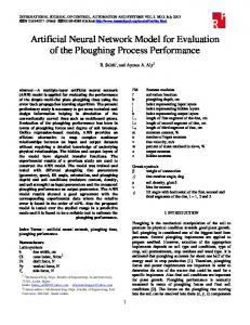
Fig. 1. Populations of ensembles and networks. Each element of the ensemble is a reference to an individual of the corresponding subpopulation of networks, together with its associated weight.

can add an objective of regularization that will encourage less complex networks without biasing the evolutionary process. The rest of the paper is organized as follows. Section II describes the proposed model of cooperative ensembles. Sections III and IV state all the aspects of network and ensemble populations and their evolution. Section V explains the multiobjective evaluation of the individuals. Section VI describes the experimental setup and Section VII shows the results of the application of our model to ten real-world problems. A comparison with standard ensemble methods is carried out in Section VIII. Sections IX and X show a comprehensive analysis of several aspects of the evolved ensembles. Finally, Section XI states the conclusions of our work and the most important lines for future research. II. COOPERATIVE ENSEMBLE OF NEURAL NETWORKS Evolutionary computation [28], [33] is a set of global optimization techniques that have been widely used in the last few years for training and automatically designing neural networks. Some efforts have been made to design modular [34] neural networks with these techniques (e.g., [35]), but the design of network ensembles by means of evolutionary computation has only been focused on some of its aspects [21], [25], [36] and not on the whole process. Cooperative coevolution [37] is a recent paradigm in the area of evolutionary computation, based on the evolution of coadapted subcomponents without external interaction. In cooperative coevolution a number of species are evolved together. Cooperation among individuals is encouraged by

rewarding the individuals for their join effort to solve a target problem. The work in this paradigm has shown that cooperative coevolutionary models present many interesting features, such as specialization through genetic isolation, generalization and efficiency [29]. Cooperative coevolution approaches the design of modular systems in a natural way, as the modularity is part of the model. Other models need some a priori knowledge to decompose the problem by hand. In many cases, either this knowledge is not available or it is not clear how to decompose the problem. So, the cooperative coevolutionary model offers a very natural way for modeling the evolution of cooperative parts. This is the case of neural network ensembles, where the accuracy of the individual networks is not enough to assure a good performance. Cooperation among individual networks is also needed in order to improve the performance significantly. Our cooperative model is based on two separate populations that evolve cooperatively. A model sharing some of these basic ideas has already been successfully applied to the evolution of modular neural networks [31]. These two populations are the following. •

Population of networks: This population consists of a number of independent subpopulations of networks. The independent evolution of subpopulations is an effective way of keeping the networks of different populations diverse. The absence of genetic material exchange among subpopulations also tends to produce more diverse networks whose combination is more effective. Every subpopulation is evolved using evolutionary programming.

274


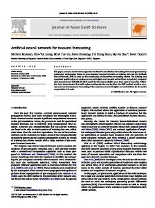
Fig. 2. Model of a GMLP.

•

Population of ensembles: Each member of the population of ensembles is an ensemble formed by a network from every network subpopulation. Each network has an associated weight. The population of ensembles keeps track of the best combinations of networks, selecting the subsets of networks that are promising for the final ensemble. The two populations evolve cooperatively. Each generation of the whole system consists of a generation of the network population followed by a generation of the ensemble population. The relationship between the two populations can be seen in Fig. 1. The second basis of our model is the use of multiobjective optimization in the evaluation of the fitness of the individual networks. We have quoted previous works that agree that the learning process of the networks must take into account the cooperation among the networks for obtaining better ensembles. Implicit cooperation among the subpopulations in cooperative coevolution helps this learning process, but it is necessary to enforce cooperation to assure good results. The evaluation of several objectives for each network allows the model to encourage such cooperation, rewarding the networks not only for their performance in solving the given problem, but also for other aspects, such as whether they are different from other networks, whether they are useful in the ensembles or anything else considered relevant by the designer. Additionally, every network is subject to back-propagation training throughout its evolution with a certain probability. In this way, the network is allowed to learn from the training set, but it is also prevented from being too similar to the rest of the networks by means of its evaluation using different objectives. The back-propagation algorithm is implemented as a mutation operator.

As we stated in Section I, many decisions must be made in order to design an ensemble of neural networks. In the next sections, we explain in depth all the aspects of our model and the decisions made, following the ideas we have already introduced. III. NETWORK POPULATION Our basic network is a generalized multilayer perceptron (GMLP), as defined in [38]. It consists of an input layer, an output layer, and a number of hidden nodes interconnected among them. hidden nodes, and outGiven a GMLP with inputs, puts, and and being the input and output vectors, respectively, it is defined by the equations [38]

(2) is the weight of the connection from node to node . where The representation of a GMLP can be seen in Fig. 2. We see that the th node, provided it is not an input node, has connections . from every th node The main advantage of using a GMLP is the parsimony of the evolved networks. Its structure allows the definition of very complex surfaces with fewer nodes than in a standard multilayer perceptron with one or two hidden layers. subpopulations. The network population is formed by Each subpopulation consists of a fixed number of networks codified directly as shown in Fig. 2. These networks are not fully connected. When a network is initialized, each connection is


created with a given probability. The population is subject to operations of replication and mutation. Crossover is not used due to potential disadvantages [39] that it has for evolving neural networks. With these features the algorithm falls in the class of evolutionary programming [40].

275

TABLE I PARAMETERS OF NETWORK STRUCTURAL MUTATIONS COMMON TO ALL THE EXPERIMENTS

A. Evolution of Networks The algorithm for the evolution of the subpopulations of networks is similar to other models proposed in the literature, such as GNARL [39] or EPNet [35]. The steps for generating the new subpopulations are the following. • Networks of the initial subpopulation are created randomly. The number of nodes of the network is obtained . Each node from a uniform distribution is created with a number of connections taken from a . uniform distribution • The new subpopulation is generated replicating the best of the previous subpopulation. The remaining is removed and replaced by mutated copies of networks selected by roulette selection from the best individuals. • There are two types of mutation: parametric and structural. The severity of structural mutation is determined by the relative fitness, , of the network. Given a network , its relative fitness is defined as (3) is the fitness value of network , and is a where parameter that must be chosen by the expert. In our ex. periments Parametric mutation consists of the modification of the weights of the network without modifying its topology. Many parametric mutation operators have been suggested in the specific literature: random modification of the weights [12], simulated annealing [35], and back-propagation [35], among others. In this paper, we use the back-propagation algorithm [38] as mutation operator. This algorithm is performed for a few iterations with a low value of the learning coefficient (in our experiments ). Parametric mutation is always carried out after structural mutation, as it does not modify the structure of the network. Structural mutation is more complex, because it implies a modification of the structure of the network. The behavioral link between parents and their offspring must be enforced to avoid generational gaps that produce inconsistency in the evolution [35], [39]. There are four different structural mutations. • Addition of a node: The node is added with no connections to enforce the behavioral link with its parent. • Deletion of a node: A node is selected randomly and deleted together with its connections. • Addition of a connection: A connection is added, with weight 0, to a randomly selected node. There are three types of connections: from an input node, from another hidden node and to an output node. The selection of the type of connection to remove is made according to the relative number of each type of nodes: input, output and hidden. Otherwise, when there is a significant difference

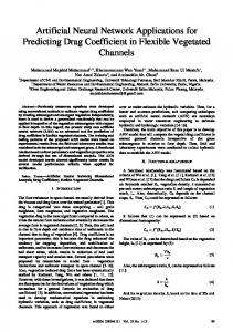
in the number of these three types, the number of connections of each type may end up highly biased. • Deletion of a connection: A connection is selected, following the same criterion of the addition of connections, and removed. All of the above mutations can be made in a single mutation operation over the network. For each mutation there is a minand a maximum value . The number of imum value elements (nodes or connections) involved in the mutation is calculated as follows: (4) So, before making a mutation, the number of elements is , the mutation is not actually carried out. calculated. If The values of network mutation parameters used in all of our experiments are shown in Table I. There is no migration among subpopulations. So, each subpopulation must develop different behaviors of their networks, that is, different species of networks, in order to compete with the other subpopulations for conquering its own niche and to cooperate to form ensembles with high fitness values. This will help the diversity among networks of different subpopulations. For the initialization of the weights of the networks, we used the method suggested by Le Cun, [2], [41]. The weights are obtained from a uniform distribution within the interval , where is the number of inputs to the network. The whole evolutionary process for network in a generation is illustrated in Fig. 3(a). The figure shows the possible evolution of a network during one generation of the evolutionary process. IV. ENSEMBLE POPULATION The ensemble population is formed by a fixed number of ensembles. Each ensemble is the combination of one network from each subpopulation of networks with an associated weight. The relationship between the two populations has been shown in Fig. 1. It is important to note that, as the chromosome that represents the ensemble is ordered, the permutation problem [39], that is so important in network evolution, cannot appear. A. Evolution of Ensembles The ensemble population is evolved using the steady-state genetic algorithm [42], [43]. It has been proved that this model shows higher variance [44] and is a more aggressive and selective selection strategy [45] than the standard genetic algorithm.

276

Fig. 3.


(a) Evolutionary process of a network and (b) an ensemble in a generation showing the possible steps of the process.

This algorithm is selected due to the fact that we need a population of ensembles that evolves more slowly than the population of networks, as the changes in the population of ensembles have a major impact on the fitness of the networks. The steady-state genetic algorithm avoids the negative effect that this drastic modification of the population of ensembles may have over the subpopulations of networks. It has also been shown by some works in the area [46], [47] that the steady-state genetic algorithm produces better solutions than the standard genetic algorithm. Crossover is made at network level, using a standard twopoint crossover. So the parents exchange their networks to generate their offspring. Mutation is also carried out at network level.1 When an ensemble is mutated, one of its networks is selected and is substituted by another network of the same subpopulation selected by means of a roulette algorithm. The whole evolutionary process for ensemble th in a generation is illustrated in Fig. 3(b). The figure shows the possible evolution of an ensemble during one generation of the evolutionary process. 1There is also a parametric mutation of the weights of the networks that is explained in Section IV-B.

During the generation of the new network population, some networks of every subpopulation are removed and substituted by new ones. The removed networks are also substituted in the ensembles. This substitution has two advantages: first, poor performing networks are removed from the ensembles and substituted by potentially better ones; second, new networks have the opportunity to participate in the ensembles immediately after their creation. B. Combination of Network Outputs Basically, in a classification environment, there are three methods for combining the outputs of the networks [6]: Majority voting, sum of the outputs of the networks, and winner takes all. The most commonly used methods for combining the networks are the majority voting and sum of the outputs of the networks, both of them with a weight vector that measures the confidence in the prediction of each network. Each network is asand the output of the ensemble is obtained signed a weight using (5)


where is the number of networks that make up the ensemble, is the output of network . The problem of obtaining and the weight vector is not trivial. Usually, the values of the weights are constrained in order to help to produce estimators with lower prediction error [48], although justification of this constraint is just intuitive [49]. In this work, we use the sum of the outputs of the network with a weight vector. The “basic ensemble method (BEM),” as it is called in [1], consists of weighting all the networks equally. So, having networks, the output of the ensembles is

277

The ambiguity of the network with respect to the ensemble . The ensemble on input is defined by ambiguity for input is given by (9) The most interesting aspect of the ambiguity is that the global error of the ensemble can be expressed in function of the error and ambiguity of each network that form the ensemble [54] (10)

(6) Perrone and Cooper [1] defined the generalized ensemble method, which is equivalent to the mean square error – optimal linear combination (MSE-OLC) without a constant term of are given by Hashem [50], where the values of (7) is the symmetric correlation matrix , where defines the misfit of func, tion , that is the deviation from the true solution . Many other techniques have been proposed in the last few years, such as, linear regression [48], principal components analysis and least-square regression [51], correspondence analysis [6], and the use of a validation set [25]. In this work, we use a genetic algorithm for obtaining the weight of each component, and not only for selecting the most interesting subsets of networks. This approach is similar to the use of a gradient descent procedure [52], avoiding the problem of being trapped in local minima. The use of a genetic algorithm has an additional advantage over the optimal linear combination, as the former is not affected by the collinearity problem [1], [50]. Our method considers each ensemble as a chromosome and applies a standard genetic algorithm to optimize the weight of each network. The weight of each network of the ensemble is codified as a real number. The chromosome formed in this way is subject to standard two-point crossover and mutation. Mutation consists of a simulated annealing [53] algorithm. where

C. Diversity Diversity is one of the key aspects of network ensembles. The error of an ensemble can be decomposed by analysis of the ambiguity of the individual networks that make up the ensemble [54]. Let us assume that we have an ensemble of networks, and . Each network has the output of network th on input is a weight that measures the confidence on such network. The is defined by output of the ensemble (8) As we have stated in the description of standard ensembles, see Section IV-B, the weights usually have the restriction of being positive and sum to one.

where , and , being the error in the network, and the average ambiguity over the generalization set. This equation shows that the error can be decreased by improving the ambiguity of the individual networks, provided that the individual error of the networks is not increased. This can be explained as another form of bias/variance decomposition [55]. Thus, the objective of any method for developing network ensembles must be obtaining accurate networks as diverse as possible. In our model, diversity is assured by means of three different mechanisms. 1) Coevolution of genetically isolated subpopulation of networks: As there is no exchange of genetic material among the members of the different subpopulations, diversity among the subpopulations is preserved. 2) Fitness-sharing in the evaluation of the networks: When a network is evaluated, we use fitness-sharing for decreasing the fitness of the networks functionally close to each other. 3) Objectives of diversity: Additionally, each network is evaluated using one or more objectives of diversity. Again, diverse networks are rewarded. The evaluation of the ensembles also includes an objective rewarding the ensembles formed by diverse networks. D. Pattern Sampling One of the aspects of neural network ensemble design that has received a lot of attention in the literature is the topic of training data set sampling. Sampling methods have shown to be successful in improving the performance of different classifiers in artificial and real-world data sets [56]–[58]. These algorithms can be divided into two types: algorithms that adaptively change the distribution of the training set, based on the performance of the previous classifiers, and algorithms that do not adapt the distribution. Boosting methods are the most representative methods of the first group. The most widely used boosting methods are Ada-Boost [59] and Arcing-x4 [60]. All of them are based on adaptively increasing the probability of sampling the patterns that are not classified correctly by the previous classifiers. Bagging [57] is the most representative algorithm of the second group. Bagging (after Bootstrap aggregating) just generates different bootstrap samples from the training set. As we are developing a cooperative model of evolution, the methods that adaptively modify the probability of selecting a pattern are not easily incorporated to the evolution. In our model

278


each network of every population receives a different bootstrap sample from the original training data set. V. MULTIOBJECTIVE EVALUATION OF NETWORK AND ENSEMBLE FITNESS If we approach the problem of evaluation of the fitness of networks and ensembles as a multiobjective optimization task, we will benefit from many advantages. First, there is no need to weight the different objectives, as would be the case using an aggregating approach. Second, the solutions based on Pareto optimality guarantee the diversity [61] of the final population. Third, there is an underlying theory applicable to our problem. In addition, it gives us a framework for adding as many objectives as may be of interest. The next two sections describe the objectives that have been defined for networks and ensembles. These are only a subset of all the objectives that may be interesting for a given task. One of the advantages of our model is that it allows the introduction of any useful objective without modifying the general structure of the system. A. Individual Networks Objectives The objectives of the networks could be grouped into four sets: objectives of performance, objectives of regularization, objectives of cooperation and objectives of diversity. We have three objectives of performance, one objective of regularization, two objectives of cooperation, and four objectives of diversity. These objectives are the following. 1) Objectives of Performance: These objectives measure the performance of the network from three different complementary points of view. The objectives are the following. • Performance: As we use bagging, this measure of performance is the number of patterns correctly classified by the network pondered by the weight of each pattern. • Shared performance: This objective enforces the networks to classify different patterns [15]. In this way, the networks that are able to accurately classify patterns that are incorrectly classified by many ensembles are rewarded. Each pattern receives a value that measures the number of ensembles that correctly classify the pattern, namely (11) where is the number of ensembles that classify the pattern correctly, and is the number of ensembles. The value assigned to a network for this objective is given by (12) where is 1 if pattern is correctly classified by the network, and 0, otherwise, and is the number of patterns. With this objective the networks that classify difficult patterns are rewarded, even if the total number of patterns correctly classified by the network is not high. This idea is similar to the theoretical basis of boosting, as boosting

also encourages the learning of difficult patterns raising their probability of being sampled. • Ensembles: Average performance of the ensembles where the network is present. In order to reward the best collaborating networks, this objective measures the average performance of the ensembles where the network participates. When a network does not participate in any ensemble, the objective cannot be calculated. In such a case the objective receives a value of 0. 2) Objectives of Regularization: In order to reward small networks, many measures may be included as regularization terms. These measures can be taken from network pruning [62], or regularization theory [32], [63]. Most authors use the weight decay term proposed in many papers [64], [65] (13) Other authors propose a cost function of the form [62] (14) nevertheless, both measures have a strong impact on the evolution of the network due to the heavy constraint that is imposed on the weights. For that reason, we have used the following less restrictive term. • Regularization objective: This term is taken from [66]. The idea is to model the weights of the network using a mixture of two Gaussians, a narrow ( ) one, and a broad ( ) one

(15) where the parameters of the distributions, , , and , are obtained by means of an expectation-maximization (EM) algorithm [67]. The effect of this regularization term is a kind of soft version of weight-sharing in which the learning process decides itself which weights should be tied together. 3) Objectives of Cooperation: These two objectives explicitly promote cooperation among the networks. Instead of evaluating the performance of networks or ensembles, these objectives evaluates the relevance of the network within the ensembles where it participates and how well it cooperates with the rest of the members of those ensembles. These two objectives for a network in a subpopulation , are the following. • Difference: The network is removed from all the ensembles where it is present, and the performance of such ensembles with the network removed is measured. The value of this criterion is measured as the difference in performance of these ensembles with and without the network. This criterion enforces competition among subpopulations of networks preventing more than one subpopulation from developing the same behavior. If two subpopulations evolve in the same way, the value of this criterion in the fitness of their networks will be near 0 and the networks will be penalized.


•

Substitution: The best ensembles of the population are selected. In these ensembles the network of subpopulation is substituted by the network . The fitness of the ensemble with the network of the subpopulation substituted by is measured. The fitness assigned to the network is the average difference in the fitness of the ensembles with the original network and with the network substituted by . This criterion enforces competition among networks of the same subpopulation, as it tests if a network can achieve a better performance than the rest of the networks of its subpopulation.

4) Objectives of Diversity: In the development of ensembles of neural networks, we must take into account the source of the error on an ensemble. The ensemble generalization error can be expressed (see Section IV-C)

•

(16) is the weighted average of the individual where is the networks’ generalization errors and weighted average of the diversity among these networks. From this point of view, the objective of any ensemble is to obtain highly correct networks that disagree as much as possible. Maintaining diversity needs some kind of speciation mechanism [68]. The most common techniques are: fitness sharing [22], [69], crowding [70], implicit fitness sharing [12], [68], local mating [71], and negative correlation [18]. Nevertheless most of these methods may bias the evolutionary process. The importance of the diversity of combined networks in an ensemble have been stated by many authors [1], [18], [21], [24]. Nevertheless, some works raise some doubts about the usefulness of diversity measures in building classifier ensembles in real-world classification problems [24]. Moreover, it is very difficult to determine which measures of diversity are the most suitable for a given task. Our approach takes advantage of the cooperative and multiobjective environment we are using. We define four objectives regarding diversity, and the evolutionary process will combine networks that are good at different objectives. The number of diversity measures is enormous, so we have selected four of the most widely used, each one centered on a different idea. These objectives are the following. •

Correlation: Following Liu and Yao [21], we introduce an objective that measures the correlation of the error of each individual network with the ensembles where it participates. The error correlation of network in an ensemble is measured using of networks

279

, that is, the average The value used as objective is error correlation of the network over all the ensembles where it is present. From both theoretical and experimental results [72] it has been shown that, if the individual networks in an ensemble are unbiased, the most effective combination of them occurs when the errors of the individual networks are negatively correlated. As a consequence, the mutual information between each individual and the rest of the population should be minimized [18] to improve the estimation of the ensemble. This idea has been used before in other papers [18], and a very similar idea is implemented in [20]. Functional diversity: Before the definition of a functional diversity measure, we defined such function axiomatically. The three axioms that a functional diversity measure , over a set , must for two functions and , fulfill are the following. . Axiom 1: Axiom 2: if and only if . . Axiom 3: Obviously, any distance measure fulfills these axioms. So, the measure we have chosen is the average Euclidean distance among the outputs of the two networks. This measure is used to test the discrepancy among the outputs of the networks. For two networks, and , the functional diversity , is defined as (18)

•

A similar measure, using a principal components analysis [73] of the outputs have been used in [12], [74]. Mutual information. The mutual information [23] between two networks, and , is given by [18] (19) where is the entropy of , and is the joint differential entropy of and . If we suppose that the output of network is a Gaussian random variable is given with variance , the differential entropy, by (20) The joint differential entropy

is given by (21)

(17)

where is the number of training patterns, is the is the output output of network for pattern , and of the ensemble for pattern . With this measure a network must learn what all other networks have not yet learned.

where is the covariance matrix of and . Following Liu et al. [18], who used this criterion for evolving a population of networks, the final form of the mutual information between the two networks is (22)

280

•


where is the correlation coefficient between and . Yule’s statistic. This objective [24] measures whether the mistakes of the classifiers are uncorrelated, and it is one of the various statistics to assess the similarity of two classifiers outputs [75]. The Yule’s statistic [76] for two and is given by classifiers (23) where

is given by

We have selected this measure, because it has been proved to be the one with the best results in a recent paper comparing ten different diversity measures [24]. Classifiers that recognize the same patterns will have positive values of , and classifiers that tend to commit mistakes in different patterns will have negative values of . B. Ensemble Objectives The same principles of multiobjective evolution can also be applied to the evolution of ensembles. So, we have defined two objectives to be considered in the evaluation of ensemble fitness. These two objectives for the ensembles are as follows. • Performance: This objective is just the performance of the network measured as the number of patterns classified correctly. • Ambiguity: As we have explained in Section IV-C, if the in-correlation among the networks that form the ensemble is increased, without increasing the individual errors, the global error of the ensemble is reduced. The ambiguity is defined over the training set. The ensembles could also be evolved taking into account just one objective, their performance in solving the given problem, but the multiobjective approach showed better results. C. Multiobjective Algorithm The multiobjective algorithm is common to both populations, networks and ensembles. We will consider a population of individuals where individual has a vector of objectives values . The population has individuals, and objectives are considered. The comparison and selection of the most suitable multiobjective algorithm is not a trivial task [77]. The proposed algorithm is based on the concept of Pareto optimality [78] and has been chosen taking into account as the most important feature the computational cost. It has common points with other multiobjective evolutionary algorithms. The multiobjective algorithm for obtaining the fitness of an individual with a vector of objecis outlined in Fig. 4. tives The comparison and selection of the most suitable multiobjective algorithm is not a trivial task [77]. This algorithm is

Fig. 4. Multiobjective evolutionary algorithm for obtaining the fitness of individuals of the population.

basically an adaptation of nondominated sorting genetic algorithm (NSGA) [79] to evolutionary programming. The idea underlying NSGA is the use of a ranking selection method to emphasize current nondominated individuals and a niching method to maintain diversity in the population. The use of second generation algorithms, such as strength Pareto evolutionary algorithm (SPEA) [80] or Pareto archive evolutionary strategy (PAES) [81], is not feasible as the concept of a separate population of nondominated individuals cannot be translated into our model. The algorithm consists of two stages. First, the successive nondominated fronts2 are obtained and every individual of these . Second, the fronts is assigned an equal dummy fitness members of every front share their fitness. The procedure must guarantee that none of the members of a front gets a higher fitness than any of the members of the previous front. The algorithm used for obtaining the nondominated set of solutions [78] compares the individuals pairwise and marks as dominated all the individuals that are dominated by at least one member of the population. Once the individuals of a nondominated front are assigned their fitness, they are not considered any more for obtaining the new nondominated front. That is the reason why we talk about successive nondominated fronts. 2A nondominated front is a subset of individuals that are not dominated by any member of the population.


The problem of fitness sharing among the members of the same Pareto front is crucial for the performance of the algorithm. The standard method of explicit fitness sharing [69] (for a discussion [82]) cannot be applied, as the individuals are not in an Euclidean space. So, we must define a measure of diversity for networks and ensembles in order to apply the algorithm. Our interest is focused on keeping behavioral diversity among the individuals, so our distance measure is based on the func, for networks, and tional diversity measure defined above, on an extension of functional diversity for ensembles. networks of the th nondominated front, Given a set of , the sharing procedure each having a dummy fitness of . The sharing is performed for each solution procedure consists of the following steps for th individual. 1) Compute the functional diversity with every individual of the Pareto front . 2) Compare this value with a predefined niche radius, and apply the sharing function if otherwise

(24)

3) Calculate niche count for individual (25) 4) Modify the fitness of the individual according to its niche count (26) For the ensemble population, we have defined an ensemble functional diversity. The measure of ensemble functional diversity is based on the functional diversity of networks. Given two ensembles and , is defined as their functional diversity (27) With this distance measure, the above sharing algorithm is applied, just substituting the measure of functional diversity for the ensemble functional diversity . VI. EXPERIMENTAL SETUP The experiments were carried out with the objective of testing our cooperative model against the most used ensemble methods. We have applied our model and standard ensemble methods to several real-world problems of classification. These problems are briefly described in Table II. These ten sets cover a wide variety of problems. There are problems with different number of available patterns, from 214 to 3175, different number of classes, from 2 to 19, different kind of inputs, nominal, binary and continuous, and of different areas

281

of application, from medical diagnosis to vowel recognition. Testing our model on this wide variety of problems can give us a clear idea of its performance. The tests were conducted following the guidelines of Prechelt [83]. Each set of available data was divided into three subsets: 50% of the patterns were used for learning, 25% of them for validation, and the remaining 25% for testing the generalization error. There are two exceptions, Sonar and Vowel problems, as the patterns of these two problems are prearranged in two subsets due to their specific features. The column network in Table II specifies the architecture of the networks used in the standard ensembles. The populations of cooperative ensembles were evolved without a validation set, adding the validation set to the training set. At the end of the evolution, the fifth best network, in terms of training error, was selected as the result of the evolution. The test set was then used for obtaining the generalization of this network. The standard ensembles used for comparison are made up of 25 networks. It is known [84] that the diversity and the accuracy of the ensemble usually plateau at some size between 10 and 50 members. Moreover, Opitz and Maclin [85] have found after some exhaustive experiments that the error of the ensemble does not decrease after adding 25 networks. For the training of the standard networks in the ensembles, we used the method of cross-validation and early stopping [86]. The networks were trained until the error over the validation set started to grow. For Ada–Boosting, it is required that the weak learning algorithm, in our case, each individual network, achieves an error strictly less than 0.5. This cannot be guaranteed especially when dealing with multiclass problems. In our experiments when this error is not achieved, we generate a bootstrap sample from the original set and continue up to a limit of 25 trials. This method has been used in previous works [17], [56]. For two problems, Soybean and Vowel, the network was not able to reach this error and Ada–Boosting could not be applied. For each data set, 30 runs of the algorithm were performed. In all the tables, we show the average error of classification over the 30 runs, the standard deviation, and the best and worst individuals. The measure of the error is the following:

(28)

where is the number of patterns, and is 0, if pattern is correctly classified, and 1, otherwise. The parameters used in our experiments are common to the ten problems. They are fairly standard as their performance is very good for the different problems we have solved. The cooperative ensembles used for all the problems are made up of ten networks, in contrast with the standard ensembles that are made up of 25 networks. We want to show how the cooperative coevolution of the networks can achieve a very good performance with a comparatively small ensemble. The population of ensembles has 100 individuals and each subpopulation of networks has 30 networks. The elitism in the population of networks is 50%.

282


SUMMARY

OF DATA SETS. THE NETWORK

TABLE II THE FEATURES OF EACH DATA SET CAN BE (C)ONTINUOUS, (B)INARY, OR (N)OMINAL. COLUMN SHOWS THE NUMBER OF (I)NPUT, (H)IDDEN, AND (O)UTPUT NODES

The parametric mutation rate in the population of ensembles is 100% and the structural mutation rate is 5%. VII. EXPERIMENTAL RESULTS The first step of our experiments was to obtain a lower limit for the performance of the model. In order to obtain such a limit, we trained a single network using the same model of the cooperative ensembles, the GMLP. It is obvious that an ensemble must be, at least, better than a single network. The results are shown in Table III. The network was not able to achieve useful results for the Soybean and Vowel problems. Once we have established a lower bound for the performance of our model, we carried out an experiment in order to test the viability of the model. From the ten test problems we have described, we chose a subset of five problems: Cancer, Glass,

Heart, Horse, and Pima. We made 30 runs for each problem, using all the objectives we have defined. The results are shown in Table IV. The performance of the model is clearly better than the results of the single network. Nevertheless, the use of the ten objectives is not very advisable, because some of the objectives share the same principles. So, we did a second experiment in order to test whether all the objectives were useful in the evolution. For two problems, Heart and Glass, we repeated the 30 runs removing each objective in turn. The results are shown in Table V. Table V shows that removing an objective only has a significant effect on the generalization error (with a 5% confidence level) in four cases in the Heart problem, and in none of them in the Glass problem. Moreover, removing the functional diversity objective has a beneficial effect over the error in the Glass


283

TABLE III ERROR RATES FOR A SINGLE NETWORK (SNG) AND STANDARD ENSEMBLES. THE t-TEST COMPARES THE AVERAGE ERROR OF THE EXPERIMENT WITH COOPERATIVE ENSEMBLES USING SIX OBJECTIVES AND THE EXPERIMENTS WITH A SINGLE NETWORK AND EACH ENSEMBLE METHOD

problem. These results showed us that the use of all the defined objectives was not the best option. That idea is also reinforced by two additional reasons. 1) The literature on multiobjective optimization shows that these algorithms do not perform successfully with so many objectives as ten [87].

2) Many of the objectives are closely related and it would be more advisable to choose a few or just one of them from each group. In order to test the relevance of each objective, we carried out another experiment over Heart and Glass data sets using every objective alone in turn. The results are shown in Table VI.

284


TABLE IV ERROR RATES USING ALL OF THE TEN OBJECTIVES

TABLE V ERROR RATES USING NINE OBJECTIVES FOR HEART AND GLASS DATA SETS. THE t-TEST COMPARES THE AVERAGE ERROR OF THE EXPERIMENT WITH TEN OBJECTIVES AND EACH EXPERIMENT USING NINE OBJECTIVES

Due to the surprisingly good performance on the Glass problem of the objectives substitution and difference alone, we performed an additional test with these objectives on the Pima data set (also, shown in Table VI). Further experimentation has

shown that substitution and difference alone are very efficient in producing low learning errors. In problems where learning and generalization errors are highly correlated, the results of these objectives alone are excellent.


285

TABLE VI ERROR RATES USING ONE OBJECTIVE FOR HEART, GLASS, AND PIMA DATA SETS. THE t-TEST COMPARES THE AVERAGE ERROR OF THE EXPERIMENTS WITH TEN OBJECTIVES AND EACH EXPERIMENT USING ONE OBJECTIVE

From these experiments, we obtain a subset of six objectives to be used for all the problems. This subset is made up of difference, substitution, ensembles, shared performance, regularization,and Yule’s . These objectives were selected with the criterion of selecting at least one objective from each group and within each group selecting the best performing one in the two previous experiments. The results for the ten problems with this subset of six objectives are shown in Table VII. The results are excellent and are among the best in the literature [4], [16], [35], [56], [85]. Table VII also shows the computational effort needed for obtaining the given results. The computational effort of an evolutionary process where all the evolutions end in success, as it is

our case, can be defined [88] as the number of evaluations of the , fitness function. We have a population of fixed size so the number of evaluations of the fitness function in generations is . In the table, we show the average number of generations of the 30 runs of each experiment. The results obtained are very good when they are compared with other works using these data sets. Table VIII shows a summary of the results reported in papers devoted to ensemble or similar classification methods. Comparisons must be made cautiously, as the experimental setup is different in many papers. There are differences also in the methods used for estimating the generalization error. Some of the papers use tenfold cross-validation that for some of the problems obtains a more optimistic

286


TABLE VII ERROR RATES USING THE SUBSET OF SIX OBJECTIVES FOR ALL THE PROBLEMS. THE COMPUTATIONAL EFFORT IS SHOWN AS THE AVERAGE NUMBER OF GENERATIONS

RESULTS

OF

TABLE VIII PREVIOUS WORKS USING THE SAME DATA SETS. WE RECORD THE RESULTS BEST METHOD AMONG THE ALGORITHMS TESTED IN EACH PAPER

estimation of the error. With these cautions, we can say that for Cancer, Glass, Heart, Pima, Sonar, Soybean, and Vowel data sets our methods achieve a performance that is better or similar to all the results reported in the cited papers. Gene and Horse results are poorer than those obtained by other papers, and card results are improved by two of the papers. As in our experiments, most of these papers use an experimental setup and a set of parameters common to all the problems.

OF THE

VIII. COMPARISON WITH STANDARD ENSEMBLE MODELS In order to assure the level of performance of the model, we made a comparison with standard ensembles of neural networks. We trained four different ensembles of neural networks, using the same individual neural network and the same back-propagation algorithm that we used for the cooperative ensemble. The four ensembles are the following.


287

TABLE IX AVERAGE SIZE OF THE EVOLUTIONARY AND NONEVOLUTIONARY ENSEMBLES. THE TABLE SHOWS NUMBER OF NETWORKS IN THE ENSEMBLE, AND THE AVERAGE SIZE OF THE ENSEMBLE AND OF EACH NETWORK. THE t-TEST COMPARES THE AVERAGE NUMBER OF NODES AND CONNECTIONS FOR ENSEMBLES AND CONSTITUENT NETWORKS

Standard (Std):

An ensemble of networks without sampling. The combination of networks is made using the generalized ensemble method (GEM) [1]. If two networks are linearly correlated, one of them is removed. Bagging (Bag): An ensemble of networks using Bagging [56]. As in standard, the combination of networks is made using GEM. Arcing (Arc): An ensemble of networks using one of the Boosting [89] methods, Arcing-x4 [56], [60]. As in previous methods, the combination of networks is made using GEM. Ada (Ada): An ensemble of networks using one of the Boosting methods, Ada-Boosting [59], [56]. The combination of networks is made following the Ada algorithm itself. For each problem, we did 30 runs with every type of ensemble. All the experimental setup was done as in the experiments with the cooperative ensemble in order to make a fair comparison. The results of these four ensemble methods are shown in Table III. Considering the overall performance, the best performing method is Ada-Boosting together with Bagging, the latter with a slightly worse performance than the former. From Table III, we can see how the cooperative ensemble is better than the four ensemble models for all the problems with a confidence level of 5%. This result is more important if we consider that the cooperative ensemble uses 10 networks against the 25 networks that form the other ensembles. It is also interesting to note that the size of the networks in the evolved ensembles is also less than the size of the corresponding networks in the standard ensembles. Table IX shows the average size of the ensembles and networks. We can see that not only the cooperative ensembles have fewer networks, but also that the con-

stituent networks are significantly smaller (with the exception of the soybean problem). IX. ANALYSIS OF THE COOPERATIVE ENSEMBLES In this section, we will study the behavior of the cooperative ensemble. In the previous section, we have assured that the model shows a dramatic reduction of generalization error when compared with standard ensembles. Here, we want to test the sensitivity of the model to the number of networks in the ensemble, the relevance of each objective and how it behaves in a bias/variance decomposition test. A. Analysis of the Effect of Ensemble Size In order to test the influence of the number of network subpopulations, that is, the size of the ensembles, we carried out experiments for Cancer, Glass, Heart, Horse, and Pima problems with 5, 10, 15, 25, and 30 subpopulations of networks. For each size we performed ten runs of the algorithm. The results are shown in Table X.3 The table shows that in some of the problems, namely, Heart and Horse, the addition of new networks to the ensemble produces an improvement in the performance of the model, but this increment is not significant and could not pay for the increased complexity of the model. We have performed and ANOVA I test in order to verify whether there are significant differences among the results obtained with different numbers of subpopulations. With a confidence level of 5% there are significant differences just in a few cases. We can assure that the generalization error is not significantly improved when more networks are added. Not surprisingly, the learning error is improved as new networks are being added to the ensemble. 3There are minor differences between Table X and Table VII, due to the fact that in this table we have only considered the first ten runs of the algorithm for the case of ten network subpopulations.

288


TABLE X ERROR RATES USING 5, 10, 15, 25, AND 30 SUBPOPULATIONS OF NETWORKS CANCER, GLASS, HEART, HORSE, AND PIMA DATA SETS.

B. Objectives Study In this section, we evaluate the relevance of each objective in the overall performance of the ensemble. We carry out two studies. First, we test the individual contribution of each objective by removing it from the evolution and evaluating the performance of the model without that objective. Second, we evaluate the capability of every objective, evolving the ensembles with every objective alone in turn. 1) Necessity Analysis: The necessity analysis evaluates how relevant each objective is for the overall performance of the model. In order to test the importance of the objectives, we re-

FOR

move every objective in turn and evolve the model using the other five objectives. The results of the evolution with five objectives for ten runs are shown in Table XI. There are some interesting effects that can be observed in these results. • As a general rule, all the objectives are useful. The error rate is in most cases worse when any of the objectives are removed. Nevertheless, the performance of the model considering five objectives is still acceptable. • The learning error decreases when the regularization term is removed, but the generalization error usually increases without this objective. So, we can conclude that the regularization term is playing its role, encouraging small net-


289

TABLE XI NECESSITY RESULTS. ERROR RATES REMOVING EVERY ONE OF THE SIX OBJECTIVES IN TURN FOR CANCER, GLASS, HEART, HORSE, AND PIMA DATA SETS. THE t-TEST COMPARES THE AVERAGE ERROR OF THE EXPERIMENT WITH SIX OBJECTIVES, ROW LABELED ALL OBJECTIVES, AND EACH EXPERIMENT USING FIVE OBJECTIVES

•

works with worse learning errors but in most cases better generalization errors. The usefulness of the diversity objective is not clear. The deletion of this objective significantly increases the generalization error only in the Glass problem. This result

agrees with the work of Kuncheva and Whitaker [24] that has raised some doubts on the use of diversity terms in the learning process. 2) Capability Analysis: The aim of capability analysis is to study the performance of every objective when it is used as the

290


TABLE XII CAPABILITY RESULTS. ERROR RRATES USING ONE OBJECTIVE FOR CANCER, GLASS, HEART, HORSE, AND PIMA DATA SETS. THE t-TEST COMPARES THE AVERAGE ERROR OF THE EXPERIMENT WITH SIX OBJECTIVES, ROW LABELED ALL OBJECTIVES, AND EACH EXPERIMENT USING ONE OBJECTIVE

only objective to be evaluated along the evolution. So, we evolve the populations considering just one of the six objectives used for the evolution of networks. The results for Cancer, Glass, Heart, Horse, and Pima data sets are shown in Table XII. The

performance of the isolated objectives shows two reasonable results. • The objectives that are focused on performance, difference, substitution, ensembles, and shared performance,


have a better performance when they are used as the only objective, in some cases they can achieve the same performance as the six objectives. • Objectives focused on other aspects of the ensembles, such as regularization or diversity, have a worse performance. These two effects are more important when we consider the learning error. For instance, for Glass, Heart, and Horse data sets, the learning error is clearly improved when using performance based objectives. On the other hand, if we consider regularization and diversity objectives the learning error is more than twice the learning error using the six objectives. C. Bias and Variance Decomposition Many of the recent papers studying neural network ensembles analyze error performance in terms of two factors: bias and variance. The bias of a learning algorithm is the contribution to the error of the central tendency when it is trained using different data, while the variance is the contribution of the error of the deviations from the central tendency. These two terms are evaluated with respect to a distribution of training sets usually obtained by different permutations of the available data. In addition, there is an irreducible error that is given by the degree to which the correct answer for a pattern can differ from that for other patterns with the same description. As this error cannot be estimated in most real-world problems, the measures of bias and variance usually include this error. Several authors have suggested different proposals for estimating the decomposition of the classification error, the bias and variance terms [49], [90], and [91]. All of them have different advantages and drawbacks, so we have used three measures in order to study the behavior of our cooperative model comprehensively (an excellent discussion of this topic can be found in [4]). are drawn from Let us assume that the training pairs, a test instance distribution , , and that the classification of pattern by means of classifier for a distribution of training . Kohavi and Wolpert [91] proposed a data sets is method where the expected zero-one error of classifier can be expressed by bias

variance

(29)

where bias

variance

(30) However, these measures of bias and variance do not measure the extent to which each of these underlying quantities contribute to error [4]. The irreducible error is included in the bias

291

term. This estimation has the valuable property that the sum of bias and variance terms equals the total error. The bias estimation of Kong and Dietterich [90] measures the probability of error of the central tendency of the learning algorithm. This measure is useful when comparing the quality of the central tendency of different classifiers, regarding other considerations as the frequency or strength of such central tendency. is given by The formulation of this measure bias bias

(31)

where the central tendency , for learner over the distribution of training data sets is the class with the greatest probability of selection for pattern by classifiers learned by from training sets drawn from , and is defined (32) Nevertheless, the estimation of the variance of Kong and Dietterich does not adequately measure the error due to the deviations from the central tendency. So, we have also used the decomposition defined by Breiman [92] bias (33) variance (34) These definitions have the advantage that the bias term is a direct measure of the contribution of the central tendency to the total error, and variance is a measure of the contribution of the deviations from the central tendency to the total error. For estimating these five measures, we have basically followed the experimental setup used in [4]. We divided our data set into four randomly selected partitions. We selected each partition in turn to be used as the test set and trained the learner with the other three partitions. This method was repeated ten times with different random partitions, making a total of 40 runs of the learning algorithm. The central tendency was evaluated as the most frequent classification for a pattern. The error was measured as the proportion of incorrectly classified patterns. This experimental setup guarantees that each pattern is selected for the test set the same number of times, and alleviates the effect that the random selection of patterns can have over the estimations. Fig. 5 shows the estimation of the bias of Kong and Dietterich for the learning algorithms used. Instead of representing the value of the bias, we have chosen a value of 1 for the estimation obtained for the cooperative ensemble and we represent the relative bias of the rest of the ensemble methods to the cooperative ensemble. Fig. 5 shows how the cooperative ensemble central tendency is always more accurate than the central tendency of the rest of the ensemble methods. This difference is more drastic in complex problems, such as Gene, Soybean, and Vowel. Fig. 6 shows the estimation of the relative bias and variance of Kohavi and Wolpert. As we have stated, the contribution of bias to error is the portion of the total error that is made by the central tendency of the algorithm. The contribution of variance is the portion of the error that is due to deviations from the central

292


Fig. 5. Comparison of relative bias as defined by Kong and Dietterich [90] for the ten data sets. A value of 1 has been chosen for the estimation obtained for the cooperative ensemble bias, and we represent the relative bias of the rest of the ensemble methods to the cooperative ensemble. The y axis represents this relative bias.

tendency. More informally, bias is the portion of classifications that are incorrect and equal to the central tendency, and variance is the portion of classifications that are incorrect and differ from the central tendency.

Fig. 6 shows that the cooperative ensemble improves the bias error in some problems. Nevertheless, there are no significant differences in bias error between the cooperative ensemble and the other methods in Cancer, Card, Heart, Horse, and Pima prob-


293

Fig. 6. Comparison of relative bias and variance as defined by Kohavi and Wolpert [91] for the ten data sets. A value of 1 has been chosen for the estimation obtained for the cooperative ensemble, and we represent the relative bias and variance of the rest of the ensemble methods to the cooperative ensemble. The y axis represents this relative bias and variance.

lems. We must also take into account that the irreducible error is included in the bias estimation in the model of Kohavi and Wolpert. On the other hand, the variance is reduced in almost all the problems. This is important, as it means that the algorithm

is less sensitive to variations in the training set, assuring a more robust learning process. We also notice, as can be expected, that Bagging is more successful in reducing variance and Ada-Boost reduces bias more frequently.

294


Fig. 7. Comparison of relative bias and variance as defined by Breiman [92] for the ten data sets. A value of 1 has been chosen for the estimation obtained for the cooperative ensemble, and we represent the relative bias and variance of the rest of the ensemble methods to the cooperative ensemble. The y axis represents this relative bias and variance.

Fig. 7 shows the relative bias and variance of Breiman. Breiman estimation is more closely related with the intuitive idea of bias and variance. In this estimation, irreducible error is shared by the two terms. Considering this estimation, the figure

shows how the cooperative ensemble reduces both bias and variance terms of error. This accomplished reduction allows us to say that the cooperative ensemble is both accurate in its central tendency and little responsive to the variations of the training set.


295

Fig. 8. Lesion study for the ten problems. It shows the average percentage of increment in generalization error when the best network is removed, on the left, or the worst network is removed, on the right. The x axis represents the number of networks removed from the ensemble, the y axis represents the increment of the generalization error in percentage when the corresponding networks are removed.

296


Fig. 9. First two principal components for every network of the best ensemble of the first run for cancer, card, heart, pima, and sonar problems.


Fig. 10.

297

Two first principal components for every network of the best ensemble of the first run for gene, glass, and horse problems.

D. Lesion Study Lesions are used in biological networks to identify functions or functional areas of the brain. Previous works [74] have used lesions to study the functionality of different parts of an evolved network. Here, we use lesions for testing the robustness of the ensembles. Once all the networks of the ensemble are evolved, we test the performance penalty of removing each network. In this way, we can evaluate the robustness of the ensemble if any of its constituent networks ceases to work. We have carried out two different experiments. In a first experiment, we have in turn the network that most contributes to

the performance of the ensemble, until the ensemble is just one network. In a second experiment, we repeated the previous steps removing the network that contributes the last to network performance. Fig. 8 shows the average generalization error over the 30 runs for the two experiments for the ten data sets. Fig. 8 shows a smooth degradation on the performance of the ensemble as the best networks are removed. Moreover, the effect of removing the worst network causes less damage, and this assures quite a robust ensemble. As could be expected, the effect of removing a network is more important in complex problems, such as Gene, Soybean, or Horse.

298


X. WHY DOES THE COOPERATIVE METHOD OUTPERFORM STANDARD ENSEMBLES?

TABLE XIII AVERAGE DISTANCE FROM THE CENTROID NETWORKS OF THE ENSEMBLE

OF THE

The experiments have shown that the cooperative ensemble is able to perform better than the standard ensemble methods. In the previous sections, we have gained some insights into the way the cooperative ensemble works. In this section, we want to study the features of the cooperative ensemble that would help to explain the reason why the performance of the cooperative ensemble is above the performance of the standard one. The explanation for this performance is not an easy task, so our objective is to make explicit some of the features of cooperation rather than to carry out an exhaustive study that is outside the scope of this paper. A. Principal Components Analysis Our first objective in this study is the visualization of the functionality of the networks. It is a well-known issue that as the networks are more different, the performance of the ensemble is increased. In order to show the functionality of a network, we follow the functional representation of a network (or node) of Moriarty and Miikkulainen [12]. In order to obtain the functional representation of a network, we calculate for each network its function vector. The steps to compute this vector are the following.

1) 2)

Initialize the function vector to nil. For each input unit of the network do: a) Set input to 1 and all the others to 0. b) Propagate the activation through the network. c) Append the output of the network to the function vector.

In this way, we produce a function vector for each output of the network. In order to represent the functionality of the network, we perform a principal component analysis of the function vectors, retaining the first two components. Following this method, we can represent each network by a point in a two-dimensional (2-D) space. The position of each network depends on its functionality, and we can consider that if two networks are closed in the 2-D space their functionality is somewhat similar. On the other hand, if two networks are separated, their functionality must be very different. Figs. 9 and 10 show the representation of the networks of the best ensemble of the first run of the algorithms for all the problems, except for soybean and vowel that are not represented due to their large number of outputs. For the standard ensemble, we have chosen the model that best performs for each problem. Figs. 9 and 10 show how the networks in the standard ensembles are more clustered, with many networks sharing similar functionality. On the other hand, the networks of the cooperative ensemble tend to be more spread, so their collaboration is more effective. In order to corroborate the previous affirmation, we have measured the dispersion of the networks represented on the figures. Table XIII shows the average distance of each network from the

centroid of the cluster made up of all the networks of the ensemble. This value can be considered a measure of the dispersion of the networks in the ensemble [93]. In the table, we show the average value of all the outputs. With networks, each one represented by a two dimensional vector the average distance is given by (35) where is the mean of the vectors that represent the networks in the ensemble. The table shows that the average distance of the networks is greater among the cooperative ensemble than the standard ensemble. This means that the networks have more varied behavior, and the efficiency of their combination should be better. Table XIII also shows the -values of a -test that compares whether the differences between the means are significant. With a confidence level of 5%, the differences are significant for Cancer, Heart, Gene, and Glass problems. B. Measures of the Diversity of the Individual Networks In order to complete the previous study of the diversity of the networks in the ensembles, we obtain the error correlation among the networks that make up the standard and cooperative ensembles. The values are shown in Table XIV. We have also obtained the value of Yule’s statistic (Table XIV) in order to test the similarity among the classifications performed by each network. As in the previous study, for the standard ensemble we have chosen the model that best performs for each problem. The -tests show that all the differences are significant. Table XIV shows that, as a general rule, the correlation among the errors of the individuals networks in the cooperative ensemble is below the correlation among the networks that form the standard ensemble. There are two exceptions, Cancer and Pima problems. For these two problems, the standard ensemble shows a smaller correlation. The value of Yule’s has the same property. This result, together with the results from principal component analysis, suggests that one of the sources of the excellent behavior of the cooperative ensemble comes from the


299

TABLE XIV MEASURES OF THE DIVERSITY OF THE INDIVIDUAL NETWORKS OF THE ENSEMBLES

TABLE XV CLASSIFICATION OF PATTERNS BY THE NETWORKS THAT MADE UP THE COOPERATIVE AND STANDARD ENSEMBLES

fact that the cooperation is able to obtain more diverse networks than the standard methods for constructing ensembles. C. Classification of Individual Patterns The last study of the networks of the ensembles concerns the patterns that each network classifies accurately. For all the 30 runs of the cooperative and standard models, we took the best ensemble and obtained the following two values. 1) For each ensemble, we obtained the average number of patterns correctly classified by its constituent networks considered alone. This value was average for the best ensemble of all the 30 runs. 2) For each ensemble, we obtained the percentage of patterns that were not correctly classified by any of its constituent

networks. This is a measure of how well the networks cover the training set. These two values for all the problems are shown in Table XV. The results are very interesting as they show some differences between the behavior of the standard and cooperative ensemble’s networks. The following differences can be noted. • As a general rule, the networks of the cooperative ensemble perform worse than the networks from the standard ensemble. This means that the former are more local in their behavior, instead of trying to classify every pattern, they specialized in some subsets of the patterns. • In most cases, the networks of the cooperative ensemble left fewer patterns inaccurately classified by all the networks. The number of patterns that are incorrectly clas-

300


sified by all networks is low, even for complex problems. In this way, the combination of the classifiers can be more effective. The -tests show that the differences are significant for all comparisons in the case of average classification, and for all comparisons in no classification, except Cancer, Gene, and Horse problems. XI. CONCLUSION In this paper, we have proposed a novel approach to ensemble design based on cooperative coevolution. The proposed model is a framework for all the steps of the design and training of network ensembles. The simultaneous evolution of all the networks that form the ensemble allows us to obtain more cooperative networks with a performance significantly above the performance of classic ensemble methods. The performance has been thoroughly tested over a set of ten real-world problems with different features. Our model has proved an excellent performance in the solution of these realworld problems. The performance obtained is among the best present in the literature. We have also performed an extensive analysis of the behavior of the model in different scenarios. Additional experiments have shown that the cooperative ensemble reduces the variance term of the error dramatically. This feature assures a learning algorithm less dependent on the training data set. The experiments have also shown a smooth degradation of the performance of the ensemble, when its networks are removed. The multiobjective evaluation of the fitness of the networks introduces the possibility of enforcing several aspects of the networks that are interesting for a better performance of the ensembles. In this work, we have proposed a set of general objectives that can be applied for any problem. However, the definition of other sets of objectives that may be adequate for a given problem might improve the performance of the model. Recent works [24] have stated that it is not clear that the use of diversity terms has a beneficial effect over the ensemble. Our results partially agree with this statement, as the performance of the model is not clearly improved, when the defined diversity objective is considered. A. Future Work The results of our model in classification greatly encourages a continuation of our research in cooperative coevolution of ensembles. One of the most natural continuations of out work is the application of the ideas of this paper to consensual networks [94]. It is also possible that the evolution of different kinds of networks on each subpopulation may generate more diverse populations with a potentiality for forming better ensembles. Arcing and Ada-Boosting methods also suggest the possibility of developing an incremental cooperative environment where new subpopulations are added when the evolution stagnates. The new subpopulations would be added following the Arcing or Ada models, that is, focusing their attention on the patterns that are less easily classified by the previous subpopulations.

ACKNOWLEDGMENT The authors would like to thank R. Moya–Sánchez for her helping in the final version of this paper. REFERENCES [1] M. P. Perrone and L. N. Cooper, “When networks disagree: Ensemble methods for hybrid neural networks,” in Neural Networks for Speech and Image Processing, R. J. Mammone, Ed. London, U.K.: Chapman & Hall, 1993, pp. 126–142. [2] S. Haykin, Neural Networks – A Comprehensive Foundation, 2nd ed. Upper Saddle River, NJ: Prentice–Hall, 1999. [3] T. G. Dietterich, “Ensemble methods in machine learning,” in Proc. 1st Int. Workshop Multiple Classifier Syst., J. Kittler and F. Roli, Eds., 2000, pp. 1–15. [4] G. I. Webb, “Multiboosting: A technique for combining boosting and wagging,” Mach. Learn., vol. 40, no. 2, pp. 159–196, Aug. 2000. [5] S. Dzeroski and B. Zenko, “Is combining classifiers with stacking better than selecting the best one?,” Mach. Learn., vol. 54, pp. 255–273, 2004. [6] C. J. Merz, “Using correspondence analysis to combine classifiers,” Mach. Learn., vol. 36, no. 1, pp. 33–58, Jul. 1999. [7] A. Fern and R. Givan, “Online ensemble learning: An empirical study,” Mach. Learn., vol. 53, pp. 71–109, 2003. [8] J. Hansen, “Combining predictors: Comparison of five meta machine learning methods,” Inf. Sci., vol. 119, no. 1–2, pp. 91–105, 1999. [9] R. Avnimelech and N. Intrator, “Booested mixture of experts: An ensemble learning scheme,” Neural Comput., vol. 11, no. 2, pp. 483–497, 1999. [10] G. Giacinto and F. Roli, “Dynamic classifier selection,” in Lecture Notes in Computer Science, vol. 1857, Proc. Multiple Classifier Syst. 2000, 2000, pp. 177–189. [11] A. J. C. Sharkey, “On combining artificial neural nets,” Connection Sci., vol. 8, pp. 299–313, 1996. [12] D. E. Moriarty and R. Miikkulainen, “Forming neural networks through efficient and adaptive coevolution,” Evol. Comput., vol. 4, no. 5, pp. 373–399, 1997. [13] P. J. Darwen and X. Yao, “Speciation as automatic categorical modularization,” IEEE Trans. Evol. Comput., vol. 1, pp. 101–108, Jul. 1997. [14] V. R. Khare, “Automatic Problem Decomposition using Co-Evolution and Ensembles,” M.S. thesis, Univ. Birmingham, Birmingham, U.K., 200. [15] Y. Liu, X. Yao, and T. Higuchi, “Evolutionary ensembles with negative correlation learning,” IEEE Trans. Evol. Comput., vol. 4, pp. 380–387, Nov. 2000. [16] X. Yao and Y. Liu, “Making use of population information in evolutionary artificial neural networks,” IEEE Trans. Syst., Man, Cybern. B, Cybern., vol. 28, no. 3, pp. 417–425, Jun. 1998. [17] Z.-H. Zhou, J. Wu, and W. Tang, “Ensembling neural networks: Many could be better than all,” Artif. Intell., vol. 137, no. 1–2, pp. 239–253, May 2002. [18] Y. Liu, X. Yao, Q. Zhao, and T. Higuchi, “Evolving a cooperative population of neural networks by minimizing mutual information,” in Proc. 2001 IEEE Congr. Evol. Comput., Seoul, Korea, May 2001, pp. 384–389. [19] B. Bakker and T. Heskes, “Clustering ensembles of neural network models,” Neural Netw., vol. 16, no. 2, pp. 261–269, Mar. 2003. [20] B. E. Rosen, “Ensemble learning using decorrelated neural networks,” Connection Sci., vol. 8, no. 3, pp. 373–384, Dec. 1996. [21] Y. Liu and X. Yao, “Ensemble learning via negative correlation,” Neural Netw., vol. 12, no. 10, pp. 1399–1404, Dec. 1999. [22] , “Simultaneous training of negatively correlated neural networks in an ensemble,” IEEE Trans. Syst., Man, Cybern. B, Cybern., vol. 26, no. 6, pp. 716–726, 1999. [23] T. M. Cover and J. A. Thomas, Elements of Information Theory, ser. Wiley series in telecommunication. New York: Wiley, 1991. [24] L. Kuncheva and C. J. Whitaker, “Measures of diversity in classifier ensembles and their relationship with the ensemble accuracy,” Mach. Learn., vol. 51, no. 2, pp. 181–207, May 2003. [25] D. W. Opitz and J. W. Shavlik, “Actively searching for an effective neural network ensemble,” Connection Sci., vol. 8, no. 3, pp. 337–353, 1996. [26] K. Tumer and J. Ghosh, “Analysis of decision boundaries in linearly combined classifiers,” Pattern Recognit., vol. 29, no. 2, pp. 341–348, 1996. [27] , “Error correlation and error reduction in ensemble learning,” Univ. Texas, Austin, TX, Tech. Rep. TX 78712–1084, 1996.


[28] D. E. Goldberg, Genetic Algorithms in Search, Optimization and Machine Learning. Reading, MA: Addison–Wesley, 1989. [29] M. A. Potter and K. A. de Jong, “Cooperative coevolution: An architecture for evolving coadapted subcomponents,” Evol. Comput., vol. 8, no. 1, pp. 1–29, 2000. [30] N. García-Pedrajas, C. Hervás-Martínez, and J. Muñoz-Pérez, “COVNET: A cooperative coevolutionary model for evolving artificial neural networks,” IEEE Trans. Neural Netw., vol. 14, pp. 575–596, May 2003. [31] , “Multiobjective cooperative coevolution of artificial neural networks,” Neural Netw., vol. 15, no. 10, pp. 1255–1274, Nov. 2002. [32] P. M. Williams, “Bayesian regularization and pruning using a Laplace prior,” Neural Comput., vol. 7, pp. 117–143, 1995. [33] Z. Michalewicz, Genetic Algorithms + Data Structures = Evolution Programs. New York: Springer–Verlag, 1994. [34] T. Caelli, L. Guan, and W. Wen, “Modularity in neural computing,” Proc. IEEE, vol. 87, pp. 1497–1518, Sep. 1999. [35] X. Yao and Y. Liu, “A new evolutionary system for evolving artificial neural networks,” IEEE Trans. Neural Netw., vol. 8, pp. 694–713, May 1997. [36] Y. Liu and X. Yao, “Negatively correlated neural networks for classification,” in Proc. 3rd Int. Symp. Artificial Life Robotics (AROBIII’98), vol. 2, M. Sugisaka, Ed., Beppu, Japan, 1998, pp. 736–739. [37] M. A. Potter, “The design and analysis of a computational model of cooperative coevolution,” Ph.D. dissertation, Goerge Mason Univ., Fairfax, VA, 1997. [38] P. J. Werbos, The Roots of Backpropagation: From Ordered Derivatives to Neural Networks and Political Forecasting. New York: Wiley, 1994. [39] P. J. Angeline, G. M. Saunders, and J. B. Pollack, “An evolutionary algorithm that constructs recurrent neural networks,” IEEE Trans. Neural Netw., vol. 5, pp. 54–65, Jan. 1994. [40] D. B. Fogel, “Evolving artificial intelligence,” Ph.D. dissertation, Univ. California, San Diego, CA, 1992. [41] Y. LeCun, L. Bottou, G. B. Orr, and K.-R Müller, “Efficient backprop,” in Neural Networks: Tricks of the Trade, G. B. Orr and K.-R. Müller, Eds. Berlin, Germany: Springer-Verlag, 1998, pp. 9–50. [42] D. Whitley and J. Kauth, “GENITOR: A different genetic algorithm,” in Proc. Rocky Mountain Conf. Artif. Intell., Denver, CO, 1988, pp. 118–130. [43] D. Whitley, “The GENITOR algorithm and selective pressure,” in Proc 3rd Int. Conf. Genetic Algorithms, M. K. Publishers, Ed., Los Altos, CA, 1989, pp. 116–121. [44] G. Syswerda, “Uniform crossover in genetic algorithms,” in Proc. 3rd Int. Conf. Genetic Algorithms, 1989, pp. 2–9. [45] D. Goldberg and K. Deb, “A comparative analysis of selection schemes used in genetic algorithms,” in Foundations of Genetic Algorithms, G. Rawlins, Ed. Sasn Mateo, CA: Morgan Kaufmann, 1991, pp. 94–101. [46] D. Whitley and T. Starkweather, “GENITOR II: A distributed genetic algorithm,” J. Experimental Theoretical Artif. Intell., pp. 189–214, 1990. [47] G. Syswerda, “A study of reproduction in generational and steady-state genetic algorithms,” in Foundations of Genetic Algorithms, G. Rawlins, Ed. Sasn Mateo, CA: Morgan Kaufmann, 1991, pp. 94–101. [48] M. Leblanc and R. Tibshirani, “Combining estimates in regression and classification,” Dept. Statistics, Univ. Toronto, Toronto, ON, Canada, Tech. Rep., 1993. [49] L. Breiman, “Stacked regressions,” Mach. Learn., vol. 24, no. 1, pp. 49–64, 1996. [50] S. Hashem, “Optimal linear combinations of neural networks,” Neural Netw., vol. 10, no. 4, pp. 599–614, 1997. [51] C. J. Merz, “A principal components approach to combining regression estimates,” Mach. Learn., vol. 36, no. 1, pp. 9–32, Jul. 1999. [52] J. Kivinen and M. Warmuth, “Exponential gradient descent versus gradient descent for linear predictors,” Inf. Comput., vol. 132, no. 1, pp. 1–63, Jan. 1997. [53] S. Kirkpatrick, C. D. Gelatt, Jr., and M. P. Vecchi, “Optimization by simulated annealing,” Science, vol. 220, pp. 671–680, 1983. [54] A. Krogh and J. Vedelsby, “Neural networks ensembles, cross validation, and active learning,” in Advanced in Neural Information Processing Systems 7, G. Tesauro, D. S. Touretzky, and T. K. Leen, Eds. Cambridge, MA: MIT Press, 1995, pp. 231–238. [55] R. Meir, “Bias, variance and the combination of estimators; The case of linear least squares,” in Advances in Neural Information Processing Systems, G. Tesauro, D. Touretzky, and T. Leen, Eds. Cambridge, MA: MIT Press, 1995, vol. 7. [56] E. Bauer and R. Kohavi, “An empirical comparison of voting classification algorithms: Bagging, boosting, and variants,” Mach. Learn., vol. 36, no. 1/2, pp. 105–142, Jul./Aug. 1999.

301

[57] L. Breiman, “Bagging predictors,” Mach. Learn., vol. 24, no. 2, pp. 123–140, 1996. [58] J. R. Quinlan, “Bagging, boosting, and c4.5,” in Proc. 13th Nat. Conf. Artif. Intell., 1996, pp. 725–730. [59] Y. Freund and R. Schapire, “Experiments with a new boosting algorithm,” in Proc. 13th Int. Conf. Mach. Learn., Bari, Italy, 1996, pp. 148–156. [60] L. Breiman, “Arcing classifiers,” Ann. Statist., vol. 26, pp. 801–824, 1998. [61] P. A. N. Bosmand and D. Thierens, “The balance between proximity and diversity in multiobjective evolutionary algorithms,” IEEE Trans. Evol. Comput., vol. 7, pp. 174–188, Apr. 2003. [62] R. Reed, “Pruning algorithms – A survey,” IEEE Trans. Neural Netw., vol. 4, pp. 740–747, 1993. [63] C. Goutte and L. K. Hansen, “Regularization with a pruning prior,” Neural Netw., vol. 10, no. 6, pp. 1053–1059, 1997. [64] PAD. C. Plaut, S. J. Nowlan, and G. E. Hinton, “Experiments in learning by back propagation,” Carnegie-Mellon Univ., Pittsburgh, Tech. Rep. CMU-CS-86-126, 1986. [65] M. Ishikawa, “A structural learning algorithm with forgetting of link weights,” Electrotechnical Lab., Tsukuba-City, Japan, Tech. Rep. TR-90-7, 1990. [66] S. J. Nowlan and G. E. Hinton, “Simplifying neural networks by soft weight-sharing,” Neural Comput., vol. 4, no. 4, pp. 473–493, 1992. [67] A. Dempster, N. Laird, and D. Rubin, “Maximum-likelihood from incomplete data via the EM algorithm,” J. Royal Statist. Soc. Ser. B, vol. 39, no. 1–38, 1977. [68] J. Horn, D. E. Goldberg, and K. Deb, “Implicit niching in a learning classifier system: Natures’s way,” Evol. Comput., vol. 2, no. 1, pp. 37–66, 1994. [69] D. E. Goldberg and J. Richardson, “Genetic algorithms with sharing for multimodal function optimization,” in Proc. 2nd Int. Conf. Genetic Algorithms, San Mateo, CA, 1987, pp. 148–154. [70] K. A. de Jong, “An analysis of the behavior of a class of genetic adaptive systems,” Ph.D. dissertation, Univ. Michigan, Ann Arbor, MI, 1975. [71] R. J. Collins and D. R. Jefferson, “Selection in massively parallel genetic algorithms,” in Proc. 4th Int. Conf. Genetic Algorithms, San Mateo, CA, 1991, pp. 249–256. [72] R. T. Clemen and R. L. Winkler, “Limits for the precision and value of information from dependent sources,” Oper. Res., vol. 33, pp. 427–442, 1985. [73] I. T. Jolliffe, Principal Components Analysis. New York: Springer–Verlag, 1986. [74] D. E. Moriarty, “Symbiotic evolution of neural networks in sequential decision tasks,” Ph.D. dissertation, Univ. Texas, Austin, TX, 1997. [75] A. Afifi and S. Azen, Statistical Analysis. A Computer Oriented Approach. New York: Academic, 1979. [76] G. Yule, “On the association of attributes in statistics,” Phil. Trans., vol. 194, pp. 257–319, 1900. [77] E. Zitzler, L. Thiele, M. Laumanns, C. M. Fonseca, and V. Grunert, “Performance assessment of multiobjective optimizers: An analysis and review,” IEEE Trans. Evol. Comput., vol. 7, pp. 117–132, Apr. 2003. [78] K. Deb, “Evolutionary algorithms for multicriterion optimization in engineering design,” in Proc. Evol. Algorithms Eng. Comput. Sci. (EUROGEN’99), Jyväskylä, Finland, May/Jun. 30/3, 1999, pp. 135–161. [79] N. Srinivas and K. Deb, “Multiobjective function optimization using nondominated sorting genetic algorithms,” Evol. Comput., vol. 2, no. 3, pp. 221–248, 1994. [80] E. Zitzler and L. Thiele, “Multiobjective evolutionary algorithms: A comparative case study and the strength Pareto approach,” IEEE Trans. Evol. Comput., vol. 3, pp. 257–271, Nov. 1999. [81] K. D. Knowles and D. W. Corne, “Approximating the nondominated front using the Pareto archived evolution strategy,” Evol. Comput., vol. 8, no. 2, pp. 149–172, 2000. [82] K. Deb and D. E. Goldberg, “An investigation of niche and species formation in genetic function optimization,” in Proc. 3rd Int. Conf. Genetic Algorithms, J. D. Schaffer, Ed., Los Altos, CA, 1989, pp. 42–50. [83] L. Prechelt, “Proben1–A set of neural network benchmark problems and benchmarking rules,” Universität Karlsruhe, Fakultät für Informatik, Karlsruhe, Germany, Tech. Rep. 21/94, 1994. [84] G. Zenobi and P. Cunningham, “Using diversity in preparing ensembles of classifiers based on different feature subsets to minimize generalization error,” in Lecture Notes in Artificial Intelligence, vol. 2167, Proc. 12th Eur. Conf. Mach. Learn. (ECML 2001), L. de Raedt and P. Flach, Eds., 2001, pp. 576–587. [85] D. Opitz and R. Maclin, “Popular ensemble methods: An empirical study,” J. Artif. Intell. Res., vol. 11, pp. 169–198, 1999.

302


[86] W. Finnoff, F. Hergert, and H. G. Zimmermann, “Improving model selection by nonconvergent methods,” Neural Netw., vol. 6, pp. 771–783, 1993. [87] C. A. Coello-Coello, “A comprehensive survey of evolutionary-based multiobjective optimization techniques,” Knowl. Inf. Syst., vol. 1, no. 3, pp. 269–308, Aug. 1999. [88] J. R. Koza, Genetic Programming II. Automatic Discovery of Reusable Programs. Cambridge, MA: MIT Press, 1994. [89] R. E. Schapire, “The strength of weak learnability,” Mach. Learn., vol. 5, no. 2, pp. 197–227, 1990. [90] E. B. Kong and T. G. Dietterich, “Error-correction output coning corrects bias and variance,” in Proc. 12th Int. Conf. Mach. Learn., A. Prieditis and J. F. Lemmer, Eds., 1995, pp. 275–283. [91] R. Kohavi and D. H. Wolpert, “Bias plus variance decomposition for zero–one loss functions,” in Proc. 13th Int. Conf. Mach. Learn., L. Saitta, Ed., 1996, pp. 275–283. [92] L. Breiman, “Bias, variance, and arcing classifiers,” Dept. Statistics, Univ. California, , Berkeley, CA, Tech. Rep. 460, 1996. [93] A. K. Jain and R. C. Dubes, Algorithms for Clustering Data. Englewood Cliffs, NJ: Prentice-Hall, 1988, Advanced Reference Series. [94] J. A. Benediktsson, J. R. Sveinsson, O. K. Ersoy, and P. H. Swain, “Parallel consensual networks,” IEEE Trans. Neural Netw., vol. 8, pp. 54–64, Jan. 1997. [95] J. Friedman, T. Hastie, and R. Tibshirani, “Additice logistic regression: A statistical view of boosting,” Ann. Statist., vol. 28, no. 2, pp. 337–407, 2000. [96] M. M. Islam, X. Yao, and K. Murase, “A constructive algorithm for training cooperative neural network ensembles,” IEEE Trans. Neural Netw., vol. 14, pp. 820–834, Jul. 2003. [97] T. G. Dietterich, “An experimental comparison of three methods for constructing ensembles of decision trees: Bagging, boosting, and randomization,” Mach. Learn., vol. 40, pp. 139–157, 2000. [98] L. Breiman, “Randomizing outputs to increase prediction accuracy,” Mach. Learn., vol. 40, pp. 229–242, 2000. [99] L. Todorovski and S. Dzeroski, “Combining classifiers with meta decision trees,” Mach. Learn., vol. 50, pp. 223–249, 2003. [100] E. Cantú-Paz and C. Kamath, “Inducing oblique decision trees with evolutionary algorithms,” IEEE Trans. Evol. Comput., vol. 7, pp. 54–68, Feb. 2003.

Nicolás García-Pedrajas (M’01) was born in Córdoba, Spain, in 1970. He received the B.S. degree in computing and the Ph.D. degree from the University of Málaga, Spain, in 1993 and 2001, respectively. His dissertation research involves the automatic design of artificial neural networks using both genetic algorithms and evolutionary programming. He is a Professor of Computer Science and Artificial Intelligence in the Department of Computing and Numerical Analysis, University of Córdoba. His current research interests include neural networks, evolutionary computation, and game playing. Dr. García-Pedrajas is a member of several technical societies including the Association for Computing Machinery (ACM), the INNS, and the IEEE Computer Society.

César Hervás-Martínez (M’98) was born in Cuenca, Spain. He received the B.S. degree in statistics and operating research from the Universidad Complutense of Madrid, Madrid, Spain, in 1978 and the Ph.D. degree in mathematics from the University of Seville, Seville, Spain, in 1986. He is a Professor of Computer Science and Artificial Intelligence, Department of Computing and Numerical Analysis, University of Córdoba, Córdoba, Spain, and an Associate Professor in the Department of Quantitative Methods, School of Economics. He is a member of other technical societies. His current research interests include neural networks, evolutionary computation, and modeling of natural systems.

Domingo Ortiz-Boyer was born in Córdoba, Spain, in 1970. He received the B.S. degree in computing and the Ph.D. degree from the University of Málaga, Spain, in 1995 and 2001, respectively. He is a Professor of Computer Science and Artificial Intelligence, Department of Computing and Numerical Analysis, University of Córdoba. His current research interests include evolutionary computation, function optimization, and nonlinear regression.

Cooperative Coevolution of Artificial Neural Network Ensembles for ...

Cooperative Coevolution of Artificial Neural Network Ensembles for ...

Suggest Documents

Cooperative Coevolution of Multi-Agent Systems - Neural Network

Bayesian Neural Network Ensembles

Cooperative Coevolution of Feed Forward Neural ...

Artificial Speciation of Neural Network Ensembles - Google Sites

Artificial Speciation of Neural Network Ensembles - Google Sites

Ensembles of Artificial Neural Networks: Analysis and

A Learning Algorithm For Neural Network Ensembles

Artificial Neural Network

Supersymmetric Artificial Neural Network

Artificial Neural Network: Assignment

application of artificial neural network

Artificial Neural Network Modeling for Sorption of

Artificial Neural Network Model for Evaluation of

design of artificial neural network architecture for

Implementation of Artificial Neural Network

Artificial Neural Network Modelling for Prediction of

Neural Network Ensembles in Reinforcement Learning

Neural Network Ensembles for Time Series Forecasting - School of

Artificial neural network for tsunami forecasting

Artificial Neural Network for Transportation Infrastructure Systems

An Artificial Neural Network Approach for Brain

Artificial Neural Network Applications for Predicting ...

Artificial Neural Network Methodology for Modeling ...

The artificial neural network for forecasting foreign