the resulting overall closed loop system is input-to-state stable and apply the ..... can be viewed as two interconnected IOS systems with outputs e and Ëvr :=.
Coordinated Path-Following Control for Nonlinear Systems with Logic-Based Communication A. Pedro Aguiar and Ant´onio M. Pascoal
Abstract— We address the problem of designing decentralized feedback laws to force the outputs of decoupled nonlinear systems (agents) to follow geometric paths while holding a desired formation pattern. To this effect we propose a general framework that takes into account i) the topology of the communication links among the agents, ii) the fact that communications do not occur in a continuous manner, and iii) the cost of exchanging information. We provide conditions under which the resulting overall closed loop system is input-to-state stable and apply the methodology for two cases: agents with nonlinear dynamics in strict feedback form and a class of underactuated vehicles. Furthermore, we address explicitly the case where the communications among the agents occur with non-homogenous, possibly varying delays. A coordinated path-following algorithm is derived for multiple underactuated autonomous underwater vehicles. Simulation results are presented and discussed.
I. I NTRODUCTION Motivated by challenging practical applications, the problem of coordinated path-following (CPF) control has recently come to the forum. See for example [1]–[4] and the references therein for an introduction to the subject and an overview of important theoretical issues that warrant consideration. The essence of the problem can be best explained by focusing on a simple mission scenario with n autonomous vehicles: given n spatial paths, derive control laws to steer the vehicles along the paths at a “common” desired speed profile, while holding a specified formation pattern. Different approaches to the solution of this and similar problems have been reported in the literature [5]–[12]. The common strategy to solve the problem of CFP is to partially decouple it into two tasks: i) path-following (PF), where the objective is to find local closed loop control laws to steer each vehicle to its assigned path at a nominal reference speed, and ii) multiple vehicle coordination, where the goal is to adjust the reference speeds of the vehicles about the desired formation speed, so as to reach formation. Presently, many schemes are available for PF control. However, the coordination problem lacks a complete solution addressing explicitly practical constraints that arise from the characteristics of the supporting inter-vehicle communication network. For example, underwater applications require that a fleet of vehicles coordinate themselves by exchanging information over low bandwidth, short range communication channels that are plagued with intermittent failures, multi-path effects, Research supported in part by projects GREX / CEC-IST (Contract No. 035223) and NAV-Control / FCT-PT (PTDC/EEA-ACR/65996/2006), FREESUBNET RTN of the CEC, and the FCT-ISR/IST plurianual funding program through the POS C Program that includes FEDER funds. The authors are with the Dept. Electrical Engineering and Computers and the Institute for Systems and Robotics, Instituto Superior T´ecnico, Av. Rovisco Pais, 1, 1049-001 Lisboa, Portugal
{pedro,antonio}@isr.ist.utl.pt
and distance-dependent delays. Currently, no CPF algorithms are known that will yield guaranteed performance in the presence of such stringent constraints occurring simultaneously. Some of these issues, however, have been partially addressed in the literature by exploiting the use of graph theory to model the topology of the underlying communication network and Lyapunov-based tools to deal with intermittent failures or switching topologies [1], [3], [4], [11]. Inspired by the above results, this paper proposes a framework for CPF that applies to a very general class of nonlinear systems and takes into account the topology of the (bidirectional) communication links among such systems, explicitly. Furthermore, the paper addresses also the fact communications among systems do not occur in a continuous manner but take place at discrete instants of time instead. As such, the results in the paper go well beyond those obtained in [1], [4] where it was tacitly assumed that the flow of information is continuous, even though it may exhibit intermittent interruptions. The main contribution of the paper lies in a new proposed control architecture that aims to reduce the frequency at which information is exchanged among the systems involved by incorporating a logic-based communication. To this effect, we borrow from and expand some of the key ideas exposed in [13], [14] where decentralized controllers for a distributed system were derived by using for each system its local state information, together with estimates of the states of the systems it communicates with. Here, we introduce the key constraint that a vehicle is only allowed to communicate with a set of immediate neighbors. With the scheme adopted, each vehicle decides when to transmit information to the neighbors by comparing its actual state with its estimate “as perceived” by the neighboring systems, and transmitting data when the “difference” between the two exceeds a certain level. Thus, the systems communicate at discrete instants of time, asynchronously. With the framework proposed, we provide conditions under which the CPF control architecture obtained by putting together path-following, coordination, and logic-based communication strategies solves the CPF problem with guaranteed stability, convergence, robustness and performance in the presence of disturbances, sensor noise, and strict communication constraints. The mathematical tools adopted borrow from graph theory and the theory of ISS systems. To illustrate the scope of the methodology proposed, we solve the CPF problem for nonlinear systems in strict feedback form and for a class of underactuated vehicles. One of the key contributions is the fact that, to the best of our knowledge, and contrary to CPF algorithms described in the literature, we address explicitly the case where the communications among systems occur with non-homogenous,
w i z i
Agent Dynamics
yi Generalized zdi(Ji) Path/Speed v Computation r i (Ji) zd
i
vr
v i
J
Ji
~ v i
ui
Path-Following
i
PFC
ri
yi
Coordination Controller
^J
j
J
Communication System i
� j � Ni
CPFCS
VEHICLE NETWORK
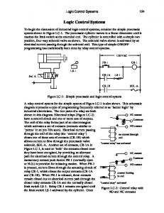
Fig. 1.
Coordinated path-following control system architecture.
possibly varying delays. Due to space limitations most of the proofs are omitted. These can be found in [15]. We refer the reader to [1]–[4] and the references therein for background material on CPF. Notation: | · | denotes the standard Euclidean norm of a vector in Rn and �u�I is the (essential) supremum norm of a signal u : [0, ∞) → Rn on an interval I ⊂ [0, ∞). We ∂z ∂2z γ2 let I := {1, . . . , n}, zdγii := ∂γdii zdii := ∂ 2 γdii , [ai ]i∈I := col(a1 , . . . , an ), and a ⊕ b := max{a, b}. II. C OORDINATED PATH -F OLLOWING C ONTROL S YSTEM This section proposes a CPF control architecture for a group of n decoupled agents Σi , i ∈ I modeled by general systems of the form Σi :
x˙ i = Fi (xi , ui , wi ), yi = Hi (xi , ui , vi ), zi = Ji (xi , ui ),
(1a) (1b) (1c)
where xi ∈ Rni denotes the state of agent i, ui ∈ Rmi its control input, yi ∈ Rpi its measured noisy output, wi an input disturbance, and vi measurement noise. The output zi ∈ Rqi is a signal that we require to reach and follow a desired feasible path zdi (γi ) : R → Rqi parameterized by γi ∈ R. The following notation � � γk is required: zdi (γi ) := col zdi (γi ), zdγii (γi ), . . . zdii (γi ) , � � γl vri (γi , t) := col vri (γi , t), vrγii (γi , t) . . . vrii (γi , t) , and (1) (n) γ i := col(γi , γi . . . γi ). The architecture for the general coordinated path-following control system (CPFCS) proposed in this paper is shown in Fig. 1. It consists of three interconnected subsystems: Path-following controller — a dynamical system whose inputs are a path zdi , a desired speed profile vri that is common to all agents, and the agent’s output yi . Its output is the agent’s input ui , computed so as to make it follow the path at the assigned speed. In preparation for its connection
to the coordination controller, this system produces also a generalized path zdi (γi ), a generalized speed profile vri (γi ), and a generalized path-variable γ i . Further, it accepts corrective speed action from the coordination controller via the signal v˜ri . Notice that the dynamics of the parameterizing variable γ i are defined internally at this stage and play the role of an extra design knob to tune the performance of the PF control law. Coordinated controller — a dynamical system whose inputs are the plant output yi , the desired generalized path zdi and speed profile vri , the generalized path-variable γ i , and estimates γ ˆ j of the generalized coordination states γ j ; j ∈ Ni where Ni , denotes the set of agents that agent i communicates with. Its output is the correction speed signal v˜ri which is used to synchronize agent i with its neighbors. Logic-based communication system — a logic-based dynamical system that establishes an interface with the network through which the agents communicate. Its inputs are the agents’ output yi , the generalized desired path zdi and speed profile vri , and the generalized path variable γ i . Its output is the estimate γ ˆ j of the generalized coordination states γ j ; j ∈ Ni . We now describe in more detail how this circle of ideas can be formalized using dynamical system concepts. We also discuss what properties every subsystem should satisfy in order to obtain a CPFCS that solves the CPF problem and is robust to input disturbances and measurement noise. A. Path-following controller Definition 1: Consider a set of n agents Σi , i ∈ I with dynamics (1) and let Zdi and Vri be the classes of admissible paths and speed profiles, respectively. We say that a given set of controllers given by ΣP F i ; i ∈ I ΣP F i : x˙ P F i = FP F i (xP F i , yi , zdi , vri , v˜ri ), ui = HP F i (xP F i , yi , zdi , vri , v˜ri )
(2a) (2b)
solves robustly the output path-following problem if for every path zdi ∈ Zdi and prescribed speed profile vri ∈ Vri , e , σve , σv˜er , σ e ∈ K∞ , β e ∈ KL and there exist functions σw a signal error e such that for each initial condition x0 := [col(xi (0), xP F i (0))]i∈I and bounded signals w := [wi ]i∈I , vri ]i∈I , all the states of the closedv := [vi ]i∈I , and v˜r := [˜ loop system (1)–(2), ∀i ∈ I with exception of γi (t) are bounded, the path-following errors ei (t) := zi (t) − zdi (γi (t)),
∀i ∈ I
and the speed errors eγ˙ i (t) := γ˙ i (t) − vri (γi , t),
∀i ∈ I
satisfy the detectability condition |ei (t)| ⊕ |eγ˙ i (t)| ≤ σ e (�e�[0,t] ),
∀i ∈ I
(3)
and e is input-to-output stable (IOS) with respect to w, v, and v˜r , that is, e |e(t)| ≤ β e (|x0 |, t) ⊕ σw (�w�[0,t] ) ⊕ σve (�v�[0,t] ) ⊕ σv˜er (�˜ vr �[0,t] ). (4)
�
B. Coordination controller Definition 2: Consider a set of n agents Σi , i ∈ I with dynamics (1), the corresponding paths zdi ∈ Zdi , and formation speed assignments vri ∈ Vr . Assume that γ i and γ j , ∀j ∈ Ni are available to agent i and let ˜ ¯ i be a bounded error signal γ ¯ i := col(γ i , [γ j ]j∈{Ni } ). Let γ ˜ γ j ]j∈Ni ). We say that a set of of the form γ ¯ i := col(0, [˜ coordination controllers ΣCCi , i ∈ I ˜ ¯i + γ ¯ i ), (5a) ΣCCi : x˙ CCi = FCCi (xCCi , yi , zdi , vri , γ ˜ ¯i + γ ¯ i ) (5b) v˜ri = HCCi (xCCi , yi , zdi , vri , γ solves robustly the coordination problem if there exist funcξ , σeξ ∈ K∞ and a coordination tions β ξ ∈ KL, σ ξ , σvξ , σγξ , σij error signal ξ that satisfies the detectability property max |γi (t) − γj (t)| ≤ σ ξ (�ξ�[0,t) )
i∈I;j∈Ni
(6)
and the evolution of ξ(t) := col(ξ, [xCCi ]i∈I , [˜ vri ]i∈I ) 0 := satisfies, for each initial condition x ξ � � col(xi (0), xP F i (0), xCCi (0)) i∈I , ˜ |ξ(t)| ≤ β ξ (|x0ξ |, t) ⊕ σvξ (�v�[0,t] ) ⊕ σγξ (�γ ¯ �[0,t] ) ⊕
ξ (�vri − vrj �[0,t) ) ⊕ σeξ (�e�[0,t) ), max σij
i∈I;j∈Ni
(7)
˜ ˜ where v := [vi ]i∈I , γ ¯ := [γ ¯ i ]i∈I and e := [ei ]i∈I .
�
C. Logic-based communication system Inspired by the communication logic proposed in [14], each communication subsystem is composed by a bank of estimators and a communication logic. The estimators run open-loop most of the time but are sometimes reset (not necessarily periodically) to correct their state when measurements are received through the network. The communication logic is responsible for determining for each agent, using an internal estimator, how well the other agents from the communication topology can predict the value of its local coordination state and decide when it should communicate the actual measured value to its neighbors. As in [14], the banks of estimators running in the different agents are synchronized, that is, the state estimate of each agent is the same as that of the corresponding neighbors. Definition 3: Consider a set of n agents Σi , i ∈ I with dynamics (1), the corresponding paths zdi ∈ Zdi , and formation speed assignments vri ∈ Vr . Assume that γ i , yi , xP F i , xCCi are continuously available to agent i and γ j ; ∀j ∈ Ni is available asynchronously through the [i] network system. Let tk ; k ≥ 0 indicate the instants of data transmission. We say that a given set of logic-based impulse dynamical systems ΣSEi ; i ∈ I defined as: [i] [i] For tk ≤ t < tk+1 xSEi , x ˆCCi , x ˆP F i , yˆi , zdi , vri , γˆi ) x ˆ˙ SEi = FSEi (ˆ ˙γˆSEi = HSEi (ˆ xSEi , x ˆCCi , x ˆP F i , yˆi , zdi , vri , γˆi )
(8a) (8b)
[i]
At t = tk+1 [i]
[i]
x ˆSEi (tk+1 ) = xSEi (tk+1 )
(9)
solves robustly the communication problem if for every i ∈ I |˜ γ j (t)| ≤ �i ,
∀j ∈ Ni , ∀t ≥ 0,
(10)
where γ ˜ j := γˆj − γ j . � At this point, for the sake of generality, we purposely avoid discussing the mechanism for generation of communication [i] times tk . This will be done later in the paper. We now state the main result of this section. Theorem 1: Consider the overall closed-loop system ΣCL composed by n agents of the form (1) and the CPFCS defined by (2), (5) and (8)–(9). Suppose that each PF controller ΣP F i and coordinated controller ΣCCi solve robustly the output path-following and coordination problem, respectively, that is, inequalities (3)–(4), (6)–(7) hold. Suppose further that the logic-based communication system satisfies (10) ∀i ∈ I and that there exists r0 ≥ 0 such that σv˜er ◦ σeξ (r) < r,
∀r > r0 .
(11)
Then, the overall closed-loop system solves robustly the CPF problem. Stated mathematically, for every agent i ∈ I, path zdi ∈ Zdi and prescribed speed profile vr = vr1 = · · · = e¯ , σve¯ ∈ K∞ , β e¯ ∈ vrn ∈ ∩i∈I Vri , there exist functions σ e¯, σw KL, a positive scalar ε, and a signal error ¯ e such that for each � � initial condition x0e := col(xi (0), xP F i (0), xCCi (0)) i∈I and bounded signals w := [wi ]i∈I and v := [vi ]i∈I , all the states of the closed-loop system ΣCL with exception of γ(t) := [γi ]i∈I are bounded, the path-following errors, speed errors, the coordination errors satisfy the detectability condition � � e�[0,t] ), (12) max |ei (t)|⊕|eγ˙ i (t)|⊕max(γi −γj ) ≤ σ e¯(�¯ i∈I
j∈Ni
and ¯ e is input-to-output practically stable (IOpS) with respect to w and v, that is, e¯ (�w�[0,t] ) ⊕ σve¯(�v�[0,t] ) ⊕ ε |¯ e(t)| ≤ β e¯(|x0e |, t) ⊕ σw (13) Proof: From (4) and (7) we conclude that the pathfollowing and coordinated controllers can be viewed as two interconnected IOS systems with outputs e and v˜r := [vri ]i∈I , respectively. An application of the small-gain theorem in [16] implies that if (11) holds then the interconnection is practically IOS. We can then conclude (13) since vri − ˜ ¯ is bounded. Inequality (12) follows using the vrj = 0 and γ detectabilities conditions (3) and (6).
III. C OORDINATED PATH - FOLLOWING FOR NONLINEAR SYSTEMS IN STRICT FEEDBACK FORM
In [17], Skjetne et al. considered the path-following problem for a nonlinear plant Σi in strict feedback form of vector relative degree ni of the form x˙ 1i = G1i (x1i )x2i + f1i (x1i ) + W1i (x1i )δ1i (t), x2i )x3i + f2i (¯ x2i ) + W2i (¯ x2i )δ2i (t), x˙ 2i = G1i (¯ .. . x˙ ni = Gni (¯ xni )ui + fni (¯ xni ) + Wni (¯ xni )δni (t), (14) yi = hi (x1i ), where xji ∈ Rmi , j = 1, . . . , ni , are the states, yi ∈ Rmi is the output, ui ∈ Rmi is the control, and δji are
unknown bounded disturbances. The matrices Gji (¯ xji ) and x1 ¯ji := hi i (x1i ) := (∂hi /∂x1i )(x1i ) are invertible for all x col(x1i , . . . , xji ), hi (x1i ) is a diffeomorphism, and Gji , fji , and Wji are smooth. The paths zdi (γi ) ∈ Zdi and speed assignments vri (γi , t) ∈ Vri considered are such that Zdi is the space of continuous uniformly bounded functions with its ni derivatives uniformly bounded on Rmi , and Vri the space of uniformly bounded functions in γi and t with their ni − 1 partial derivatives uniformly bounded in γi and t. In this section we illustrate the CPF controller architecture for a group of n agents with dynamics (14). We will use the results in [17] for the PF controller. A. Path-following controller Following the design in [17], the nth i step of backstepping yields a closed-loop system of the form xni , γi , t)χi + bi (¯ xn−1i , γi , t)ωi χ˙ i = Ai (¯ + Wi (¯ xni , γi , t)∆ni (t), γ˙ i = vri (γi , t) − ωi , where χi ∈ Rni mi is a set of new variables that include the path-following error, ∆ni := col(δ1i , . . . , δni ), ωi is an input signal to be designed, and the functions Wi ∈ Rni mi ×ni mi and bi ∈ Rni mi are uniformly bounded in their arguments. From the backstepping design described in [17] it can be concluded that for every given constant ρi > 0 we can choose sufficiently large gains such that the matrix Ai ∈ Rni mi ×ni mi satisfies � ρi � � ρi �� + Ai + Pi Ai + Pi ≤ −Qi (15) 2 2 for some matrices Pi = Pi� > 0 and Qi = Q�i > 0. We now modify the design in [17] to satisfy (3)–(4). Set ¯i, ωi = v˜ri + ω
(16)
where ω ¯ i is a feedback term to be designed such that ¯ i are the tracking update ω ¯ i → 0 as t → ∞. Examples of ω law, gradient update law, or filtered-gradient update law as described in [17], that is, i) ω ¯ i = 0, xni , γi , t), µi ≥ 0 ii) ω ¯ i = −µi τni (¯ iii) ω ¯˙ i = −λi (ρi ω ¯ i + µi τni (¯ xni , γi , t)),
λi , µi ≥ 0
where τni (¯ xni , γi , t) is the ni th tuning function defined in [17, equation (35)]. From the results in [17], property (15), vri − ω ¯ i we conclude the following and the fact that eγ˙ = −˜ Lemma. Lemma 1: The state-feedback controllers proposed in [17], together with (16) solve robustly the path-following problem and inequalities (3)–(4) hold with e := [χi ]i∈I for ¯ i )]i∈I the tracking and gradient update law or e := [col(χi , ω for the filtered-gradient update law, v ≡ 0, and w := [∆ni ]i∈I . Moreover, for fixed r, the term σv˜er (r) satisfies � lim|ρ|→∞ σv˜er (r) = 0, where ρ := [ρi ]i∈I . Remark 1: In (16), we impose relative degree one from γi to v˜ri . Other designs are possible. See [15] for the case of relative degree two.
B. Coordinated controller This section details the development of the coordination controller subsystem. To this effect, we first recall some key concepts from algebraic graph theory. Let Ni be the index set of the vehicles that vehicle i communicates with (the so called neighboring set of vehicle i). We assume that the communication links are bidirectional, that is, i ∈ Nj ⇔ j ∈ Ni . Let G(V, E) be the undirected graph induced by the inter-vehicle communication network, with V denoting the set of n nodes (each corresponding to an agent) and E the set of edges (each standing for a data link). We say that G is connected when there exists a path connecting every two nodes in the graph. The adjacency matrix of a graph, denoted A, is a square matrix with rows and columns indexed by the nodes such that the i, j-entry of A is 1 if j ∈ Ni and zero otherwise. The degree matrix D of a graph G is a diagonal matrix where the i, i-entry equals |Ni |, the cardinality of Ni . The Laplacian of a graph is defined as L := D−A. Thus, L is symmetric and its every row sums equal zero, that is, L1 = 0, where 1 := [1]n×1 and 0 := [0]n×1 . If G is connected, L has a simple eigenvalue at zero with an associated eigenvector 1 and the remaining eigenvalues are all positive. Consider now the coordination control problem with a communication topology defined by a graph G. Using a Lyapunov-based design, we propose a decentralized feedback law for v˜ri as a function of the information obtained from the neighboring agents. Following [4], we introduce the error vector 1 ξ := LK γ, LK := I − � −1 11� K −1 , 1K 1 where γ := [γi ]i∈I , 1 := [1]i∈I , and K > 0 is a diagonal matrix. See in [4], [15] some key properties of the error vector ξ. With the path-following proposed above, the dynamics of the coordination subsystem can be written in vector form as ¯, γ˙ = vr + v˜r + ω
(17)
where vr := [vri ]i∈I , ω ¯ := [ωi ]i∈I , and v˜r := [˜ vri ]i∈I . Consider the control Lyapunov function V := 12 ξ � K −1 ξ. Computing its time-derivative yields V˙ = ξ � K −1 LK (vr + v˜r + ω ¯ ). To make ξ ISS with respect to inputs LK vr and ω ¯ , and assuming that measurements of the coordination states γj ; ∀j ∈ Ni are available continuously, a natural choice would be v˜r = −KLξ = −KLLK γ = −KLγ. In this case, the dominator of V˙ , −ξ � K −1 LK KLξ = −ξ � Lξ, is negative definite provided that the Graph that models the constraints imposed by the communication topology among the agents is connected. To reduce the communication rate using a logic-based dynamical system, we will lift the assumption that each agent receives information from its neighborhoods continuously. We assume instead that it relies on estimated values. In this case, the coordination feedback law becomes γ ), (18) v˜r = −K(Dγ − Aˆ � or equivalently, v˜ri = −ki j∈Ni γi − γˆj , (the so-called neighboring rule) where ki denotes the ith diagonal element
of Ki . In (18), D and A denote the degree and adjacency matrices of the graph G, respectively. The time-derivative of V1 is V˙ 1 = −ξ � Lξ + ξ � K −1 LK (vr + ω ¯ ) + ξ � K −1 LK KA˜ γ, where γ˜ := γˆ − γ. Provided that G is connected, it is now straightforward to conclude that ξ is ISS with respect to the ¯ , and γ˜ . inputs LK vr (which is zero if vr1 = · · · = vrn ), ω This leads to the following result. Lemma 2: The coordination law (18) solves robustly the coordination problem. Inequalities (6)–(7) hold with v ≡ 0, ˜ γ ¯ = γ˜ , vri = vri , and σeξ (r) ≡ 0 for the tracking update law. For the gradient and filtered-gradient update laws the term σeξ (r) satisfies, for fixed r, limk→∞ σeξ (r) = 0, where � k := mini∈I ki .
where τ¯ > 0 is a small value known a priori. Loosely speaking, this assumption means that the time-delays in consecutive communications in a bidirectional link are roughly the same. We now describe the communication system, which is slightly different from the one in the case of non-delayed information. Due to the presence of nonhomogeneous and time-varying delays, each agent i must have |Ni | internal and synchronized estimators, that is, one set of estimators per each communication link. For example, if agent i can only communicate with agents j and �, i.e. Ni = {j, �}, then the internal estimator of agent i consists of the following systems:
C. Logic-based communication system [i]
1) No delayed information: Let tk , k ≥ 0 denote the instants of time at which agent i transmits or receives data from its neighborhoods. Following the procedure described in Section II and taking account the dynamic equations of the coordination subsystem, we propose for each agent i the following logic-based communication system: [i] [i] - For tk ≤ t < tk+1 Internal estimator: Synchronized estimators: ˆ γˆ˙ i = vˆri + vˆ ˜ri + ω ¯i vˆ˙ ri = 0 ˆ ω ¯˙ = 0 i
ˆ ˆ ˆri + v ˜ ri + ω ¯i γˆ˙ i = v v ˆ˙ ri = 0 ˆ ω ¯˙ = 0 i
(19a) (19b) (19c)
[i]
- For t = tk+1 ˆ γˆi = γi , vˆri = vri , ω ¯i = ω ¯i, ˆ γˆi = γ i , v ˆri = vri , ω ¯i = ω ¯i � where vˆ ˜ri = −ki j∈Ni γˆi − γˆj , γˆi := [ˆ γj ]j∈Ni , v ˆri := ˆ ˆ ˆ ˜ ri := [vˆ ˜rj ]j∈Ni , and ω ¯ i := [ω ¯ j ]j∈Ni . To simplify [ˆ vrj ]j∈Ni , v the estimators, we have chosen (19b)–(19c) instead of using a copy of the corresponding dynamics models. To solve robustly the communication problem (see Definition 3) we γi ) := ci γ˜i2 , ci > 0, introduce the communication index Si (˜ γ˜i := γˆi − γi and use the following logic: agent i transmits ¯i} to its neighborhoods a message by {γi , vri , ω � composed � [i] at time tk when limt↑t[i] Si γ˜i (t) ≥ 1. Note that the postk
[i]
reset value of γ˜i is γ˜i (tk ) = 0. Consequently, γ˜i ∈ {˜ γi ∈ R : S(˜ γi ) ≤ 1} and, hence, (10) holds. 2) Delayed information: We now consider the case where the communication channels have time-varying and nonhomogeneous delays. The delays are not known a priori but we assume that all the agents have synchronized clocks. Thus, each agent can compute the time-delay when the time-tagged data arrives. Consider the following situation: agent i sends [i] [i] data to j at time tk , and agent j receives it at time tk + τkij . [j] [i] Then, immediately afterwards, at time tk = tk + τkij , agent ij j sends to i the computed time-delay τk . Agent i receives [j] [i] it at time t = tk + τkji = tk + τkij + τkji . We assume that |τkji − τkij | ≤ τ¯,
∀i, ∀j ∈ Ni , ∀k ≥ 0
[�] [�] ˆ γˆ˙ i = vˆr[�]i + vˆ˜r[�]i + ω ¯i , vˆ˙ r[�]i = 0, ˆ¯˙ [�] = 0. ω
[j] ˆ¯ i[j] , γˆ˙ i = vˆr[j]i + vˆ˜r[j]i + ω vˆ˙ r[j]i = 0, ˆ¯˙ [j] = 0, ω i
i
The communication logic must also to be changed: Suppose [i] that at time tk agent i transmits to agent � a message, which [i] [i] [i] [i] contains the following data: {tk , γi (tk ), vri (tk ), ω ¯ i (tk )}. [�] Then, the internal estimator γˆi cannot be immediately updated. This is because we must guarantee that the value [�] of the state estimate γˆi will always remain equal to the corresponding state estimate running in agent �. To this effect, both estimates can only be updated at time t = [i] tk + τ¯ki� , where τ¯ki� := 2τki� + τ¯, because although agent [i] � receive the data at time t = tk + τki� , agent i only knows [i] the delay τki� at time t = tk + τki� + τk�i . Upon receiving τki� , [�] the coordination state estimate γˆi running in agent i and the corresponding dual estimate running in agent � should [i] be updated at time t = tk + τ¯ki� to [�]
[i]
[i]
γˆi (tk + τ¯ki� ) = e−2|Ni |ki (τk +¯τ ) γi (tk ) � t[i] τki� k +¯ � [i] i� [i] [i] � + e−2|Ni |ki (tk +¯τk −σ) vri (tk ) + ω ¯ i (tk ) dσ i�
[i]
tk
(20)
With the above procedure, we guarantee that the estimators are always synchronized. Equation (20) follows from (17) [�] [i] and (18). Notice that in general γ˜i (tk + τ¯ki� ) will not be ¯ i may not be constant in the interval zero because vri and ω [i] [i] [tk , tk + τ¯ki� ). The estimation error γ˜i viewed by agent � will be i� � t[i] k +2τk −1 lim γ˜i (t) = Si (1) + (21) γ˜˙ i (σ) dσ, [i]
t↑tk +¯ τki�
[i]
tk
which is bounded assuming that the time-delay is bounded, hence, (10) holds. Equation (21) only holds if the weight [�] γi ) is selected to be suffiof the communication index Si (˜ ciently small so as to guarantee that the post-reset value of γi ) < 1. γ˜i satisfies Si (˜ D. Stability analysis Using the results in Lemmas 1–2, the properties of the communication system described above, and applying Theorem 1 we conclude the following result.
Theorem 2: Consider the overall closed-loop system ΣCL composed by n agents of the form (14) and the proposed CPF controller. For sufficiently large path-following control gains or coordination control gains, the overall closed-loop system solves robustly the CPF problem. In the presence of delayed information, this result holds true for sufficiently small timedelays or weights of the communication indexes. � Remark 2: For the particular case of the path-following controller with ω ¯ = 0 (tracking update law), it turns out that the CPF controller takes a cascaded form of two ISS systems, where the output of the coordination subsystem is the input of the PF controller. In this case, there is no need to use the small-gain theorem and, hence, no constraints on the gains are required. IV. C OORDINATED PATH - FOLLOWING FOR A CLASS OF UNDERACTUATED VEHICLES
Consider an underactuated vehicle modeled as a rigid body subject to external forces and torques. Let {I} be an inertial coordinate frame and {B} a body-fixed coordinate frame whose origin is located at the center of mass of the vehicle. The configuration (R, p) of the vehicle is an element of the Special Euclidean group SE(3) := SO(3) × R3 , where R ∈ SO(3) is a rotation matrix that describes the orientation of the vehicle by mapping body coordinates into inertial coordinates, and p ∈ R3 is the position of the origin of {B} in {I}. Denoting by v ∈ R3 and ω ∈ R3 the linear and angular velocities of the vehicle relative to {I} expressed in {B}, respectively, the following kinematic relations apply: p˙ = Rv,
R˙ = RS(ω),
(22)
3
where S(·) is a function from R to the space of skewsymmetric matrices S := {M ∈ R3×3 : M = −M � }. We consider here underactuated vehicles with dynamic equations of motion of the following form: (23a) Mv˙ = −S(ω)Mv + fv (v, p, R) + gv uv Jω˙ = −S(v)Mv − S(ω)Jω + fω (v, ω, p, R) + Gω uω (23b) where M ∈ R3×3 and J ∈ R3×3 denote constant symmetric positive definite mass and inertia matrices; uv ∈ R and uω ∈ R3 denote the control inputs, which act upon the system through a constant nonzero vector gv ∈ R3 and a constant nonsingular matrix1 Gω ∈ R3×3 , respectively; the terms −S(ω)Mv in (23a) and −S(v)Mv −S(ω)Jω in (23b) are the rigid-body Coriolis terms, and the C 1 functions fv (·), fω (·) represent all the remaining forces and torques acting on the body. For the special case of an underwater vehicle, M and J also include the so-called hydrodynamic addedmass MA and added-inertia JA matrices, respectively, i.e., M = MRB + MA , J = JRB + JA , where MRB and JRB are the rigid-body mass and inertia matrices, respectively. In [18] we proposed a solution to the path-following problem for underactuated autonomous vehicles described by (22)–(23) in the presence of possibly large modeling parametric uncertainty. If we select the same update law for γ¨i as in [18] but adding the additional term v˜ri , the coordination subsystem 1 See
[18, Remark 4] for the special case of Gω ∈ R3×2 .
can be written in vector form as γ¨ = fγ (χ, γ, γ) ˙ + v˜r ,
(24)
where fγ (·) represents right-hand-side of the path-following update law in [18]. The following result holds. Lemma 3: The state-feedback controller proposed in [18] together with (24) solve robustly the path-following problem with condition (4) modified to an IOpS inequality. Moreover, if all the control gains are scaled by a factor ρ > 0, then, for fixed r, the gain function σv˜er (r) satisfies limρ→∞ σv˜er (r) = 0. � From (24), following steps similar to the ones described in [15] for the coordination, it is straightforward to obtain a decentralized feedback law of the form � γ )) , v˜r = −K(Dγ˙ − Aγˆ˙ ) − K2 (γ˙ − vr 1 + K(Dγ − Aˆ (25) where K > 0 and K2 > 0 are diagonal matrices, and to conclude that it solves robustly the coordination problem. Further, for fixed r, limk2 →∞ σeξ (r) = 0. We can now conclude the following. Theorem 3: Consider the overall closed-loop system ΣCL composed by n underactuated vehicles of the form (22)– (23) and the CPF controller with the PF control law in [18] together with (24), the coordinated controller (25), and a robustly logic-based communication system as defined in Definition 3. For sufficiently large path-following control gains or coordination control gains, the overall closed-loop system solves robustly the CPF problem. � A. CFP of underwater vehicles in 3-D space Consider an ellipsoidal shaped underactuated autonomous underwater vehicle (AUV) not necessarily neutrally buoyant. Let {B} be a body-fixed coordinate frame whose origin is located at the center of mass of the vehicle and suppose that we have available a pure body-fixed control force τu in the xB direction, and two independent control torques τq and τr about the yB and zB axes of the vehicle, respectively. The kinematics and dynamics equations of motion of the vehicle can be written as (22)–(23) (see [18] for details). Computer simulations were done to illustrate the performance of the CPF controller proposed, when applied to a group of three AUVs (n = 3). The numerical values used for the physical parameters match those of the Sirene AUV (see details in [15]). The AUVs are required to follow paths of the form � � 2π pdi (γi ) = ci cos( 2π T γi + φd ), ci sin( T γi + φd ), dγi , with c1 = 20 m, c2 = 15 m, c3 = 25 m, d = 0.05 m, T = 400, and φd = − 3π 4 . The initial conditions are p1 = (10 m, −15 m, −5 m), p2 = (5 m, 0 m, 0 m), p3 = (20 m, −25 m, 5 m), R1 = R2 = R3 = I, and v1 = v2 = v3 = ω1 = ω2 = ω3 = 0. The reference speed was set to vr = 1[sec−1 ]. The vehicles are also required to keep a formation pattern that consists of having them aligned along a common horizontal line. Furthermore, AUV 1 is allowed to communicate with AUVs 2 and 3, but the latter two do not communicate between themselves directly. To further illustrate the behavior of the proposed CPF control
−10
z [m]
0 10 20 25
30
20 15
−20
10
−10
5 0
0
−5
10
−10 −15
20
−20
R EFERENCES
x [m]
y [m]
Path−following error Coordination error
Fig. 2. Coordinated path-following of 3 AUVs, with logic-based communication. 30
30
20 10 0
0
50
100
150
0
50
100
150
0
50
100
150
200
250
300
350
400
200
250
300
350
400
200
250
300
350
400
time [s]
20 10 0
time [s]
1.5
σ
1 0.5 0 −0.5
time [s]
following). The architecture takes explicitly into account the topology of the communication links among the agents, the fact that communications do not occur in a continuous manner, and the cost of exchanging information. Conditions under which the overall closed loop system is input-tostate stable were derived. The methodology proposed was illustrated for two cases: agents with nonlinear dynamics in strict feedback form, and a class of underactuated vehicles. The problems that arise when communications among the agents occur with non-homogenous, possibly varying delays was also addressed. In this case, it was required that all the agents have synchronized clocks. Future research will aim at relaxing this requirement.
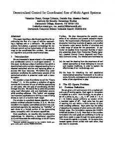
Fig. 3. Path-following error, coordination error |γ1 − γ2 | + |γ1 − γ3 |, and communication signal σ.
architecture, we also force the following scenario: from t = 150 s to t = 250 s, AUV 1 can only follow the path with γ˙ 1 = 0.1. Figure 2 shows the trajectories of the AUVs and �3 Fig. 3 the evolution of the overall path-following error i=1 �pi −pdi �, coordination error |γ1 −γ2 |+|γ1 −γ3 |, and the communication signal σ. The signal σ ∈ {0, 1} indicates, by switching its value, when there is communication. Before t = 150 s, the vehicles adjust their speeds to meet the formation requirements and the coordination errors converge to zero. Note the reduced number of communications exchanged during that period. In fact, the vehicles only need to communicate a few times during the transient phase. When AUV 1 is forced to slow down from t ∈ [150, 250] (without transmitting explicitly to its neighborhoods its new reference velocity), the communication rate increases in order to keep the coordination error bounded. V. C ONCLUSIONS We proposed a general decentralized control architecture to address the problem of forcing the outputs of decoupled nonlinear systems (agents) to follow geometric paths while holding a desired formation pattern (coordinated path-
[1] R. Ghabcheloo, A. P. Aguiar, A. Pascoal, C. Silvestre, I. Kaminer, and J. Hespanha, “Coordinated path-following control of multiple underactuated autonomous vehicles in the presence of communication failures,” in Proc. IEEE Conf. Decision and Control (CDC), San Diego, CA, USA, Dec. 2006. [2] R. Ghabcheloo, A. Pascoal, C. Silvestre, and I. Kaminer, “Nonlinear coordinated path following control of multiple wheeled robots with bidirectional communication constraints,” Int. J. Adapt. Control Signal Process, vol. 21, pp. 133–157, 2007. [3] I.-A. F. Ihle, M. Arcak, and T. I. Fossen, “Passivation designs for synchronization of path following systems,” in Proc. 45th IEEE Conference on Decision and Control, San Diego, USA, Dec 2006. [4] R. Ghabcheloo, A. Aguiar, A. Pascoal, C. Silvestre, I. Kaminer, and J. Hespanha, “Coordinated path-following in the presence of communication losses and time delays,” Submitted for publication, 2006. [5] F. Giuletti, L. Pollini, and M. Innocenti, “Autonomous formation flight,” IEEE Control Systems Magazine, vol. 20, no. 6, pp. 34–44, Dec. 2000. [6] D. J. Stilwell and B. E. Bishop, “Platoons of underwater vehicles,” IEEE Control Systems Magazine, vol. 20, no. 6, pp. 45–52, Dec. 2000. ¨ [7] P. Ogren, M. Egerstedt, and X. Hu, “A control lyapunov function approach to multiagent coordination,” in Proc. of the 40th Conf. on Decision and Contr., Orlando, FL, USA, 2001. [8] A. Jadbabaie, J. Lin, and A. S. Morse, “Coordination of groups of mobile autonomous agents using nearest neighbor rules,” IEEE Trans. on Automat. Contr., vol. 48, no. 6, pp. 988–1001, June 2003. [9] J. A. Fax and R. M. Murray, “Information flow and cooperative control of vehicle formations,” IEEE Trans. on Automat. Contr., vol. 49, no. 9, pp. 1465–1476, Sept. 2004. [10] R. Olfati-Saber and R. M. Murray, “Consensus problems in networks of agents with switching topology and time-delays,” IEEE Trans. on Automat. Contr., vol. 49, no. 9, pp. 1520–1533, Sept. 2004. [11] L. Moreau, “Stability of multiagent systems with time-dependent communication links,” IEEE Transactions on Automatic Control, vol. 50, no. 2, pp. 169–182, Feb. 2005. [12] W. Ren, R. W. Beard, and E. M. Atkins, “A survey of consensus problems in multi-agent coordination,” in Proc. of the 2005 Amer. Contr. Conf., Portland, OR, USA, June 2005. [13] J. K. Yook, D. M. Tilbury, and N. R. Soparkar, “Trading computation for bandwidth: Reducing communication in distributed control systems using state estimators,” IEEE Trans. Contr. Syst. Technol, vol. 10, no. 4, pp. 503–518, 2002. [14] Y. Xu and J. P. Hespanha, “Communication logic design and analysis for networked control systems,” in Current trends in nonlinear systems and control, L. Menini, L. Zaccarian, and C. T. Abdallah, Eds. Boston: Birkh¨auser, 2006. [15] A. P. Aguiar and A. Pascoal, “Coordinated path-following control for nonlinear systems with logic-based communication,” Institute for Systems and Robotics, Lisbon, Portugal, Tech. Rep., Sept. 2007. [16] Z. P. Jiang, A. Teel, and L. Praly, “Small-gain theorem for ISS systems and applications,” Math. Control, Signals and Systems, vol. 7, pp. 95– 120, 1994. [17] R. Skjetne, T. I. Fossen, and P. Kokotovi´c, “Robust output maneuvering for a class of nonlinear systems,” Automatica, vol. 40, no. 3, pp. 373– 383, 2004. [18] A. P. Aguiar and J. P. Hespanha, “Trajectory-tracking and pathfollowing of underactuated autonomous vehicles with parametric modeling uncertainty,” IEEE Trans. on Automat. Contr., vol. 52, no. 8, pp. 1362–1379, Aug. 2007.