as part of the Autonomous Ocean Sampling Network (AOSN) ... sign of sampling networks during the course of operation in response to ..... where fs0 = fsN = 0 .
Coordinated Patterns on Smooth Curves Fumin Zhang and Naomi Ehrich Leonard Department of Mechanical and Aerospace Engineering Princeton University { fzhang, naomi}@princeton.edu
Abstract— We show methods that control cooperative Newtonian particles to generate patterns on smooth curves. The spacing between neighboring particles is measured by the relative arc-length and the distance between a particle and the desired curve is measured using an orbit function. The orbit value and the relative arc-length are then used as feedback to control the motion of each particle to a pattern on the desired curve asymptotically. Possible applications of the methods to underwater mobile sensor networks are discussed.
function to achieve invariant patterns for N particles. We prove the convergence of the controlled dynamics to the desired pattern. In Section V, we present some simulation results.
I. I NTRODUCTION
¨r = f
Technological advances make it possible today to use fleets of sensor-equipped autonomous underwater vehicles (AUVs) to collect oceanographic data in efficient and intelligent ways never before available. For example, throughout August 2003, as part of the Autonomous Ocean Sampling Network (AOSN) field experiment, as many as twelve underwater gliders were used at once to collect data near Monterey Bay, California. This data was assimilated into ocean models that computed real-time predictions of the coupled physical and biological dynamics in the Monterey Bay region. The data set produced in August 2003 is uniquely rich and revealing [1]. Adaptive sampling refers to the ability to modify the design of sampling networks during the course of operation in response to measurements and real-time model estimation and predictions. Critical to successful adaptive sampling is the coordination of the multiple vehicles (mobile sensors) that make up the network. For instance, if the vehicles get too close to one another they may become redundant as sensors. In order to get the greatest advantage from the fleet, the vehicles should share information on their whereabouts and their observations and cooperate to best meet sampling objectives. More details can be found in a recent paper [2] and the references therein. In August 2006 in Monterey Bay, ten or more gliders will be coordinated to move on patterns that will be adapted in response to changes in the ocean and in model sensitivity. This field experiment is part of the Adaptive Sampling and Prediction (ASAP) project [3]. In this paper, we present analytical results on achieving desired patterns on closed curves using a Newtonian particle model for the idealized vehicles. In Section II, we show that the particle model can be rewritten as a system under speed and steering control. In Section III, the interaction between a controlled particle and a family of closed curves is studied. In Section IV, we derive a control law based on a Lyapunov
where r ∈ R2 and f is the total external force. The state of a particle is (r, r˙ ). If r˙ does not vanish, then we can define a unit vector x = r˙ / k r˙ k. We define � � 0 −1 y= x. (2) 1 0
To Appear in 2006 IEEE International Conference on Networking, Sensing and Control (ICNSC2006)
II. PARTICLE M ODEL In this paper, our interest is in the motion of the center of mass (COM) of a vehicle moving in the plane. We consider each vehicle as a Newtonian particle that obeys (1)
Such y is a unit vector perpendicular to x. Therefore f can be expressed as f = α2 uy + vx (3) where we define α = k r˙ k, α2 u = f · y and v = f · x. On the other hand, we compute ¨r =
d (αx) = αx ˙ + αx˙ dt
(4)
which implies that α˙ + αx˙ · x = f · x = v αx˙ · y = f · y = α2 u .
(5)
The derivative of x can be computed as follows: x˙ =
d r˙ f f ·x = − x = αuy . dt k r˙ k α α
(6)
We substitute x˙ given by (6) into equations (5) to get α˙ = v. The time derivative of y is � � 0 −1 y˙ = (αuy) = −αux . 1 0
(7)
(8)
We conclude that if the speed α of a Newtonian particle is non-zero, then the motion of the particle can be described as r˙ x˙ y˙ α˙
= = = =
αx αuy −αux v.
(9)
The advantage of using these equations instead of equation (1) comes from the fact that u can be viewed as the steering control and v can be viewed as the speed control. We note that even if we let α = 0 in equations (9), the system appears to agree with Newton’s equation (1) if f does not vanish i.e. v 6= 0. However, we have to choose x = f / k f k. In this case there might exist discontinuities in the orientation of the frame formed by x and y. III. PARTICLE AND C LOSED C URVES Suppose we are given a family of closed regular curves C(σ, z) with σ and z functions in the plane satisfying the following conditions: D1) There exists a bounded open set B such that all curves in C belongs to B and any point in B belongs to a unique curve in C. D2) z is a C 2 smooth function. On the set B, the value of z is bounded below by a real number zmin and bounded above by zmax > zmin i.e. z ∈ (zmin , zmax ). The closed curves in C are the level curves of function z. We further assume that k ∇z k = 6 0 on the set B. We call z the orbit function. D3) There exists a regular curve Γ that intersects each curve in C at a unique point. We call these intersections the starting points. D4) σ is the curve length parameter for a unique curve in C measured from the starting point. One example of such a family is the family of ellipses given by rx2 + e ry2 = z where e > 0 is the eccentricity of the ellipses (see Figure 1). If we select zmin > 0 and zmax to be a finite number greater than zmin then this family satisfies the assumptions D1) and D2) with 2
B = {(rx , ry ) ∈ R |zmin
0, zmin < czi < zmax and 0 < csj < 2π. We design control laws for (ui , vi ) so that from an arbitrary initial configuration, the particles achieve a given pattern asymptotically. Our control laws are based on control Lyapunov functions. We let hzi (z) be a smooth function on (zmin , zmax ) and hzi fzi (z) = ddz satisfying the following conditions: A1) limz→zmin hzi (z) = limz→zmax hzi (z) = +∞ A2) fzi (z) is a monotone increasing smooth function with fzi (z) = 0 if and only if z = czi . Function fzi (z) can be constructed as � � π(2z − zmax − zmin ) fzi (z) = tan − � 2(zmax − zmin ) � π(2czi − zmax − zmin ) tan . (25) 2(zmax − zmin ) We let hsj (Φ) be a smooth function on (0, 2π) and dh fsj (Φ) = dΦsj satisfying the following conditions: A3) limΦ→0 hsj (Φ) = limΦ→2π hsj (Φ) = +∞
A4) fsj (Φ) is a monotone increasing smooth function with fsj (Φ) = 0 if and only if Φ = csj . We let ha (α) be a smooth function on (0, +∞) and fa (α) = d ha dα satisfying the following conditions: A5) limα→0 ha (α) = limα→+∞ ha (α) = +∞ A6) fa (α) is a monotone increasing smooth function with fa (α) = 0 if and only if α = cv . Without loss of generality, we assume that the curve corresponding to z1 = cz1 has the minimum length among the curves determined by cz . Intuitively, in order to maintain the invariant pattern, the particle indexed by 1 on this shortest curve has to travel at the minimum speed among all particles. We will justify this intuition later. Consider the following Lyapunov candidate function: � � N X φi + hzi (zi ))+ V = (− log cos2 2 i=1 N −1 X αj+1 2 1 αj − ) )+ (hsj (Φj − Φj+1 ) + ( 2 Lj Lj+1 j=1 ha (α1 ) . (26) This Lyapunov function candidate is based on the Lyapunov function for boundary tracking and obstacle avoidance for a single vehicle first proposed in [4]. We make extensions by introducing the coupling terms controlling relative separation and speed between vehicles. This function is designed so that the invariant pattern defined by (24) is a critical point. We will show that V remains finite if V is initially finite and thus φi can never be π for all i = 1, 2, ..., N and Lj can never be 0 for all j = 1, 2, ..., N − 1. We want to compute the time derivative of the Lyapunov function along the controlled system trajectory. To simplify the process, we compute the time derivatives of each term in equation (26) separately. We also use fzi and fsj as abbreviated notations for fzi (zi ) and fsj (Φj − Φj+1 ). First, similar to [4] and [5] � � � � d 2 φi − log cos + hzi (zi ) dt 2 αi sin φ2i = [κ1i cos φi + κ2i sin φi − ui − cos φ2i φi 2fzi k ∇zi k cos2 ] 2 αi sin2 φ2i αi sin φ2i = −µ1 + u ¯i , (27) cos φ2i cos φ2i where we let for i = 1, 2, ..., N , φi + κ1i cos φi + 2 φi κ2i sin φi − 2fzi k ∇zi k cos2 − ui 2 and µ1 > 0 is a constant. Next, for j = 1, 2, ..., N − 1, � � d 1 αj αj+1 2 hsj (Φj − Φj+1 ) + ( − ) dt 2 Lj Lj+1 u ¯i
= −µ1 sin
(28)
=
� αj αj+1 vj vj+1 ˙ ˙ (Φj − Φj+1 )fsj + ( − ) − + Lj Lj+1 Lj Lj+1 2 αj ∂Lj k ∇zj k sin φj − L2j ∂zj ! 2 αj+1 ∂Lj+1 k ∇zj+1 k sin φj+1 . (29) L2j+1 ∂zj+1
We let for i = 1, 2, ..., N , v¯i = vi +
αi2 ∂Li k ∇zi k sin φi . Li ∂zi
(30)
Then for j = 1, 2, ..., N − 1 � � αj d αj+1 2 hsj (Φj − Φj+1 ) + ( − ) dt Lj L� j+1 � αj αj+1 v¯j v¯j+1 ˙ ˙ = (Φj − Φj+1 )fsj + ( − ) − . (31) Lj Lj+1 Lj Lj+1 Notice that Φ˙ j � − Φ˙ j+1 αj+1 αj cos φj − cos φj+1 − = 2π Lj Lj+1 � αj Pj αj+1 Pj+1 k ∇zj k sin φj + k ∇zj+1 k sin φj+1 L� Lj+1 j αj+1 αj+1 αj αj φj φj+1 + − − − 2 sin2 2 sin2 = 2π Lj Lj+1 Lj 2 Lj+1 2 � αj Pj αj+1 Pj+1 k ∇zj k sin φj + k ∇zj+1 k sin φj+1 (32) Lj Lj+1 for j = 1, 2, ..., N − 1. Furthermore, if we add equations (27) and (31) and sum over i and j, the following term appears and can be simplified as follows: N −1 � N X X αi sin φ2i αj αj+1 φj φj+1 u ¯i + − 2 sin2 + − 2 sin2 φi Lj 2 Lj+1 2 cos 2 j=1 i=1 � αj Pj αj+1 Pj+1 k ∇zj k sin φj + k ∇zj+1 k sin φj+1 2πfsj Lj Lj+1 N X αi sin φ2i [¯ ui − = cos φ2i i=1 � � 1 Pi 2 φi 2π(fsi − fs(i−1) ) sin φi + 2 k ∇zi k cos ] (33) Li Li 2 where fs0 = fsN = 0 . We let for i = 1, 2, ..., N , � � 1 Pi φi u ¯i = 2π(fsi − fs(i−1) ) sin φi + 2 k ∇zi k cos2 Li Li 2 (34) so that equation (33) vanishes. Then V˙ =
N X
(−µ1
i=1 N −1 � X j=1
αi sin2
φi 2
cos φ2i
αj αj+1 − Lj Lj+1
) + fa (α1 )v1 +
��
�
v¯j v¯j+1 − + 2πfsj . (35) Lj Lj+1
We let for j = 1, 2, ..., N − 1, v¯j v¯j+1 − + 2πfsj = −µ2 Lj Lj+1
�
αj αj+1 − Lj Lj+1
� (36)
and v1 = −µ3 fa (α1 )
(37)
where µ2 > 0 and µ3 > 0. Then V˙ =
N X
(−µ1
αi sin2
φi 2
cos φ2i −µ3 fa (α1 )2 ≤ 0 . i=1
)−
N −1 X j=1
� µ2
αj+1 αj − Lj Lj+1
�2 (38)
We summarize our control laws for i = 1, 2, ..., N and j = 1, 2, ..., N − 1 as follows: φi ui = κ1i cos φi + κ2i sin φi − 2fzi k ∇zi k cos2 − 2 � � 1 Pi 2 φi 2π(fsi − fs(i−1) ) sin φi + 2 k ∇zi k cos Li Li 2 φi −µ1 sin 2 v1 = −µ3 fa (α1 ) α2 ∂Li vi = v¯i − i k ∇zi k sin φi Li ∂zi � � v¯j+1 αj+1 v¯j αj − = −2πfsj − µ2 − . (39) Lj Lj+1 Lj Lj+1 It is easy to check that our Lyapunov function V has compact sub-level sets. Under the feedback control laws defined by (39), starting in the compact sub-level set determined by the finite initial value of the function V, the system equations given by (22) are Lipschitz continuous in the sub-level set and piecewise Lipschitz continuous with respect to time. Therefore a solution exists and is unique. Since the value of the Lyapunov function is time-independent and non-increasing, we conclude that if the initial value of V is finite, then the entire solution stays in the sub-level set so that V is finite for all time. This and conditions A3) and A5) imply that along such a solution, the speed of the first particle satisfies α1 > 0 and the phase differences satisfy Φj − Φj+1 6= 0 for j = 1, 2, ..., N − 1. Applying Theorem 4.4 on page 192 in [6], we conclude that as t → ∞, the controlled system converges to the set where V˙ = 0. This set is equivalent to αj αj+1 φi = 0, α1 = cv and = (40) Lj Lj+1 where i = 1, 2, ..., N and j = 1, 2, ..., N − 1. On this set, α1 ≤ αi because L1 ≤ Li for i = 1, 2, ..., N . In order to show that the controlled dynamics converges to the invariant pattern given by (24), we use the facts that φ˙ i → 0 and � � αj+1 d αj − → 0. (41) dt Lj Lj+1 To prove these facts, notice that under the control laws given in (39) � � � � d αj αj αj+1 αj+1 − = −2πfsj − µ2 − . (42) dt Lj Lj+1 Lj Lj+1 We know that fsj (Φj −Φj+1 ) is a smooth function on (0, 2π). Furthermore, as a function of t, Φj − Φj+1 is bounded in the compact sub-level set determined by the finite initial
value of the Lyapunov function. Therefore, fsj is a uniformly continuous function with respect to t. On the other hand, � � α α is also a smooth and bounded function in µ2 Ljj − Lj+1 j+1 the compact sub-level � � set. Hence as the solution of equation α α (42), Ljj − Lj+1 is a uniformly continuous function of t. j+1 Therefore, the right hand side of equation (42) is uniformly continuous with respect to time. Since we know that � � αj αj+1 − →0 (43) Lj Lj+1 as t → +∞, by the Barbalat lemma we conclude that for j = 1, 2, ..., N − 1 � � αj+1 d αj − → 0. (44) dt Lj Lj+1
Fig. 2. The initial positions of the three vehicles and the desired superelliptic track. The horizontal axis and the vertical axis indicates the longitude and latitude values respectively.
This further implies that fsj → 0. Thus according to property A4) we conclude that Φj − Φj+1 → csj .
(45)
Let us now study the equation for φ˙ i , φ˙ i = αi (κ � 1i cos φi + κ2i sin φi − ui ) φi φi + 2fzi k ∇zi k cos2 + = αi µ1 sin 2 2 � �� 1 Pi φi 2π(fsi − fs(i−1) ) sin φi + 2 cos2 . (46) Li Li 2 As t → +∞, since φi (t) → 0 and fsi → 0, we have lim φ˙ i (t) = lim (2αi fzi k ∇zi k).
t→+∞
t→+∞
(47)
Since k ∇zi k and fzi are smooth functions on a compact sublevel set of V , they are all bounded. Their time derivatives are bounded because z˙ is bounded on the compact sub-level set. Thus they are uniformly continuous. As proved in [7], ˙ an extension of the Barbalat lemma claims that φ(t) → 0 ˙ because φ(t) converges to a uniformly continuous function and φ(t) → 0. Therefore, we conclude that as t → +∞, fzi → 0. Using property A2), we have zi → czi for i = 1, 2, ..., N . Notice that all our arguments are based on the assumptions that αi (t) 6= 0 for i = 2, 3, ..., N (with α1 (t) 6= 0 guaranteed by the finiteness of the Lyapunov function). These assumptions are not very difficult to be satisfied if the initial speed for each of the particles is large enough and the desired speed for the first particle is also large enough. We have observed convergence in simulations even if αi = 0 for some i. However, to justify this observation we need to use nonsmooth system theory. In summary, we have proved the following proposition. Proposition 4.2: Consider an invariant pattern given by (cz , cs , cv ) and (24). Assume that conditions A1)-A6) and D1)-D4) hold and the initial conditions of N Newtonian particles in the plane are such that the initial value of V given by (26) is finite. Suppose further that αi (t) 6= 0 for all t and i = 1, 2, ..., N . Then, the invariant pattern is achieved asymptotically by the system of N particles under the control laws (39).
Fig. 3. The three vehicles move counter-clockwise on the desired 40km by 16km super-elliptic track.
V. S IMULATIONS AND APPLICATIONS Our control laws will be applied to coordinate a mobile sensor network for ocean sampling. One class of closed curves that will play an important role in the upcoming ASAP field experiment in August 2006 is the class of super-ellipses. A super-ellipse looks like a rectangular box with rounded corners. Oceanographers who operate AUVs are interested in the super-ellipse because large segments of the curve are almost straight lines. In addition, the almost rectangular shape allows one to easily divide a large region into smaller rectangular blocks. As ocean dynamics change, an AUV can be directed from patrol of the boundary curve of the large block to patrol of the smaller block. We simulate such a scenario in a region near Monterey Bay, CA where the ASAP field experiment will be held. In the first example, three vehicles are controlled to patrol a 40km by 16km super-elliptic box. Furthermore, vehicles 1 and 2 and vehicles 2 and 3 should be separated along the track such that Φ1 − Φ2 = Φ2 − Φ3 = cs1 = cs2 = π/2. The minimum speed for the vehicles is cv = 1km per hour. Figure 2 shows the initial positions of the vehicles and Figure 3 shows the controlled configuration at time equal to 62.5 hours. After 80 hours, we control vehicles 1 and 3 to be on a smaller 12km by 4.8km box while vehicle 2 stays on the larger box. The separations between vehicles 1 and 2 as well as between
Fig. 4. The vehicles 1 and 3 move on a 12km by 4.8km super-elliptic box and vehicle 2 moves on the 40km by 16km box.
Fig. 6. The separation between vehicles 1 and 2, Φ1 − Φ2 , as a function of time.
measurement noise affect the performance of the control laws. VI. S UMMARY
Fig. 5. The orbit value z1 , which is the length of the semi-major axis, as a function over time.
vehicles 2 and 3 are still controlled to cs1 = cs2 = π/2 as shown in Figure 4. In this case vehicles 1 and 3 travel at lower speed than vehicle 3. After 140 hours, the vehicles are commanded to resume the original pattern on the larger box. Figure 5 shows the value of the orbit function z1 of vehicle 1 as a function of time. The value of the orbit function is the length of the semi-major axis of the super-ellipse that the vehicle instantly occupies. Figure 6 shows the separation Φ1 − Φ2 between vehicles 1 and 2 over time. From these figures, one can observe the asymptotic convergence under the control laws. It can be seen that it takes less than 20 hours to set up the pattern on the larger box and about 30 hours to transit from this pattern to the second pattern with vehicles 1 and 3 on the smaller box. The time required for the vehicles to set up the sensor network is long mainly because the vehicles are slow and the boxes are large. This is generally the case for underwater gliders. Traveling at 1km per hour, it takes a vehicle 40 hours to cover the long side of the large box. In our simulation, the initial conditions for the vehicles are arbitrarily given. However, in the field experiments, by other methods such us time optimal control, we will set up the initial configurations to be close enough to the desired configuration and the control laws will maintain the network under disturbances. We are currently studying how the disturbances caused by ocean flow, positioning error and
We have shown an approach for achieving invariant patterns for mobile sensor networks. In this paper, the patterns obtained are on tracks which serve as the planned paths for the vehicles. Our approach may also have applications in using multiple sensor platforms to detect and survey natural boundaries. Other recent methods for this purpose can be found in [8], [9] and [10]. In those papers coherent patterns are established using methods that are different from ours. Our approach has provided a general theoretical frame work in developing means for systematic pattern generation on closed curves. VII. ACKNOWLEDGMENT The authors want to thank R. E. Davis and D. M. Fratantoni for discussions on controlling underwater gliders for adaptive sampling, I. Shulman and P. Lermusiaux for discussions and sharing ocean model fields and D. Paley and J. Pinner for discussions and help with simulation software. This work was supported in part by ONR grants N00014–02–1–0826, N00014–02–1–0861 and N00014–04–1–0534. R EFERENCES [1] Autonomous Ocean Sampling Network. [Online]. Available: http: //www.mbari.org/aosn/ [2] P. Bhatta, E. Fiorelli, F. Lekien, N. E. Leonard, D. A. Paley, F. Zhang, R. Bachmayer, R. E. Davis, D. M. Fratantoni, and R. Sepulchre, “Coordination of an underwater glider fleet for adaptive sampling,” in Proc. International Workshop on Underwater Robotics, Genoa, Italy, 2005, pp. 61–69. [3] Adaptive Sampling and Prediction (ASAP) Project. [Online]. Available: http://www.princeton.edu/∼dcsl/asap/ [4] F. Zhang, E. Justh, and P. S. Krishnaprasad, “Boundary following using gyroscopic control,” in Proc. of 43rd IEEE Conference on Decision and Control. Atlantis, Paradise Island, Bahamas: IEEE, 2004, pp. 5204– 5209. [5] F. Zhang and N. Leonard, “Generating contour plots using multiple sensor platforms,” in Proc. of 2005 IEEE Symposium on Swarm Intelligence, Pasadena, California, 2005, pp. 309–314. [6] H. Khalil, Nonlinear Systems, 2nd Ed. New Jersey: Prentice Hall, 1995. [7] A. Micaelli and C. Samson, “Trajectory tracking for unicycle-type and two-steering-wheels mobile robots,” INRIA report 2097, 1993.
[8] A. L. Bertozzi, M. Kemp, and D. Marthaler, “Determining environmental boundaries: Asynchronous communication and physical scales,” in Cooperative Control, A Post-Workshop Volume: 2003 Block Island Workshop on Cooperative Control, V. Kumar, N. Leonard, and A. Morse, Eds. Springer, 2005, pp. 35–42. [9] J. Clark and R. Fierro, “Cooperative hybrid control of robotic sensors for perimeter detection and tracking,” in Proc. 2006 American Control Conference, Portland,OR, June 6-10, 2005, pp. 3500–3505. [10] M. A. Hsieh and V. Kumar, “Pattern generation with multiple robots,” submitted to 2006 International Conference on Robotics and Automation, 2005.