Coordination in Multiagent Reinforcement Learning - Semantic Scholar

DRAFT VERSION OF PAPER, to appear, 2nd Intl. Conf. on Autonomous Agents and Multiagent Systems (AAMAS-03)

Coordination in Multiagent Reinforcement Learning: A Bayesian Approach Georgios Chalkiadakis

Craig Boutilier

Department of Computer Science University of Toronto Toronto, ON, M5S 3H5, Canada

Department of Computer Science University of Toronto Toronto, ON, M5S 3H5, Canada

[email protected]

[email protected]

ABSTRACT Much emphasis in multiagent reinforcement learning (MARL) research is placed on ensuring that MARL algorithms (eventually) converge to desirable equilibria. As in standard reinforcement learning, convergence generally requires sufficient exploration of strategy space. However, exploration often comes at a price in the form of penalties or foregone opportunities. In multiagent settings, the problem is exacerbated by the need for agents to “coordinate” their policies on equilibria. We propose a Bayesian model for optimal exploration in MARL problems that allows these exploration costs to be weighed against their expected benefits using the notion of value of information. Unlike standard RL models, this model requires reasoning about how one’s actions will influence the behavior of other agents. We develop tractable approximations to optimal Bayesian exploration, and report on experiments illustrating the benefits of this approach in identical interest games.

1.

INTRODUCTION

The application of reinforcement learning (RL) to multiagent systems has received considerable attention [18, 14, 4, 9, 3]. However, in multiagent settings, the effect (or benefit) of one agent’s actions are often directly influenced by those of other agents. This adds complexity to the learning problem, requiring that an agent not only learn what effects its actions have, but also how to coordinate or align its action choices with those of other agents. Fortunately, RL methods can often lead to coordinated or equilibrium behavior. Empirical and theoretical investigations have shown that standard (single-agent) RL methods can under some circumstances lead to equilibria [18, 4, 10, 3], as can methods designed to explicitly account for the behavior of other agents [14, 4, 9]. Multiagent reinforcement learning (MARL) algorithms face difficulties not encountered in single-agent settings: the existence of multiple equilibria. In games with unique equilibrium strategies (and hence values), the “target” being learned by agents is well-defined. With multiple equilibria, MARL methods face the problem that agents must coordinate their choice of equilibrium (and not just their ac-

Permission to make digital or hard copies of all or part of this work for personal or classroom use is granted without fee provided that copies are not made or distributed for profit or commercial advantage and that copies bear this notice and the full citation on the first page. To copy otherwise, to republish, to post on servers or to redistribute to lists, requires prior specific permission and/or a fee. Copyright 2002 ACM X-XXXXX-XX-X/XX/XX ...$5.00.

tions).1 Empirically, the influence of multiple equilibria on MARL algorithms is often rather subtle, and certain game properties can make convergence to undesirable equilibria very likely [4]. For obvious reasons, one would like RL methods that converge to desirable (e.g., optimal) equilibria. A number of heuristic exploration strategies have been proposed that in fact increase the probability (or even guarantee) that optimal equilibria are reached in identical interest games [4, 13, 12, 19]. Unfortunately, methods that encourage or force convergence to optimal equilibria often do so at a great cost. Coordination on a “good” strategy profile often requires exploration in parts of policy space that are very unrewarding. In such a case, the benefits of eventual coordination to an optimal equilibrium ought to be weighed against the cost (in terms of reward sacrificed while learning to play that equilibrium) [1]. This is simply the classic RL exploration-exploitation tradeoff in a multiagent guise. In standard RL, the choice is between: exploiting what one knows now about the effects of actions and their rewards by executing the action that—given current knowledge— appears the best; and exploring to gain further information about actions and rewards that has the potential to change the action that appears best. In the multiagent setting, this tradeoff exists with respect to action and reward information. But another aspect comes to bear: the influence one’s action choice has on the future action choices of other agents. In other words, one can exploit one’s current knowledge of the strategies of others, or explore to try to find out more information about those strategies. In this paper, we develop a model that accounts for this generalized exploration-exploitation tradeoff in MARL. We adopt a Bayesian, model-based approach to MARL, much like the single-agent model described in [5]. Value of information will play a key role in determining an agent’s exploration policy. Specifically, the value of an action consists of two components: its estimated value given current model estimates, and the expected decision-theoretic value of information it provides (informally, the ability this information has to change future decisions). We augment both parts of this value calculation in the MARL context. The estimated value of an action given current model estimates requires predicting how the action will influence the future action choices of other agents. The value of information associated with an action includes the information it provides about other agents’s strategies, not just the environment model. Both of these changes require that an agent possess some model of the strategies of other agents, for which we adopt a Bayesian view [11]. Putting these together, we derive optimal exploration methods for (Bayesian) multiagent systems. After reviewing relevant background, and describing related work 1 The existence of multiple equilibria can have a negative impact on known theoretical results for MARL [9, 10].


in MARL, we develop a general Bayesian model, and describe certain computational approximations for optimal exploration. We describe a number of experiments illustrating this approach, with our experiments focusing on identical interest games, since these have has been the almost exclusive target of recent research on heuristic exploration methods.

2.

BACKGROUND

We begin with basic background on RL and stochastic games.

2.1 Bayesian Reinforcement Learning We assume an agent learning to control a stochastic environment modeled as a Markov decision process (MDP) hS, A, R, Pri, with finite state and action sets S, A, reward function R, and dynamics Pr. The dynamics Pr refers to a family of transition distributions Pr(s, a, ·), where Pr(s, a, s0 ) is the probability with which state s0 is reached when action a is taken at s. R(s, r) denotes probability with which reward r is obtained when state s is reached.2 The agent is charged with constructing an optimal Markovian policy π : S 7→ A that maximizes the expected sum of future discounted rewards t t 0 over an infinite horizon: Eπ [ ∞ t=0 γ R |S = s]. This policy, and its value, V ∗ (s) at each s ∈ S, can be computed using standard algorithms such as policy or value iteration. In the RL setting, the agent does not have direct access to the model components R and Pr. As such, it must learn a policy based on its interactions with the environment. Any of a number of RL techniques can be used to learn an optimal policy π : S 7→ A. We focus here on model-based RL methods, in which the learner maintains an estimated MDP hS, A, R, Pri, based on the set of experiences hs, a, r, ti obtained so far. At each stage (or at suitable intervals) this MDP can be solved exactly, or approximately. Bayesian methods in model-based RL allow agents to incorporate priors and explore optimally. We assume some prior density P over possible dynamics D and reward distributions R, which is updated with each data point hs, a, r, ti.3 Letting H denote the (current) state-action history of the observer, we use the posterior P (D, R|H) to determine an appropriate action choice at each stage. The formulation of [5] renders this update tractable by assuming a convenient prior. Specifically, the following assumptions are made: (a) the density P is factored over R and D; (b) P (D) is the product of independent local densities P (Ds,a ) for each transition distribution Pr(s, a, ·); and (c) each density P (Ds,a ) is a Dirichlet.4 To model P (Ds,a ) we require a Dirichlet parameter vector ns,a 0 with entries ns,a,s for each possible successor state s0 . The expec0 tation of Pr(s, a, s0 ) w.r.t. P is given by ns,a,s / i ns,a,si . Update of a Dirichlet is a straightforward: given prior P (Ds,a ; ns,a ) is the number of observed transiand data vector cs,a (where cs,a i tions from s to si under a), the posterior is given by parameter vector ns,a + cs,a . Thus the posterior P (D|H) over transition models can be factored into posteriors over local families, each of the form:

P

The Bayesian approach has several advantages over other approaches to model-based RL. First, it allows the natural incorporation of prior knowledge. Second, approximations to optimal Bayesian exploration can take advantage of this model [5]. We elaborate on optimal exploration below in the MARL context.

2.2 Stochastic Games and Coordination A normal form game is a tuple G = hα, {Ai }i∈α , {Ui }i∈α i, where α is a collection of agents, Ai is the set of actions available to agent i, and Ui is agent i’s payoff function. Letting A = ×Ai denote the set of joint actions, Ui (a) denotes the real-valued utility obtained by i if the agents execute a ∈ A. We refer to any σi ∈ ∆(Ai ) as a mixed strategy. A strategy profile σ is a collection of strategies, one per agent. We often write σi to refer to agent i’s component of σ, and σ−i to denote a reduced strategy profile dictating all strategies except that for i. We use σ−i ◦ σi to denote the (full) profile obtained by augmenting σ−i with σi . Let σ−i be some reduced strategy profile. A best response to σ−i is any strategy σi s.t. Ui (σ−i ◦ σi ) ≥ Ui (σ−i ◦ σi0 ) for any σi0 ∈ ∆(Ai ). We define BR(σ−i ) to be the set of such best responses. A Nash equilibrium is any profile σ s.t. σi ∈ BR(σ−i ) for all agents i. Nash equilibria are generally viewed as the standard solution concept to games of this form. However, it is widely recognized that the equilibrium concept has certain (descriptive and prescriptive) deficiencies. One important problem (among several) is the fact that games may have multiple equilibria [8], leading to the problem of equilibrium selection. As an example, consider the simple two-player identical interest game called the penalty game [4], shown here in standard matrix form:

bc

P

P (Ds,a |H s,a ) = α Pr(H s,a |Ds,a )P (Ds,a )

(1)

where H s,a is the subset of history involving s, a-transitions and updates are of the Dirichlet parameters. 2 We will treat this distribution as if it has support over a finite set of possible values r, but more general density functions can be used. 3 We write D for the family of distributions for notational clarity. 4 We assume reward densities are modeled similarly, with a Dirichlet prior over reward probabilities for each s. Dearden et al. [5] allow for Gaussian reward distributions, which incurs no serious complications.

b0 b1 b2

a0 10 0 k

a1 0 2 0

a2 k 0 10

Here agent A has moves a0, a1, a2 and B has moves b0, b1, b2. The payoffs to both players are identical, and k < 0 is some penalty. There are three pure equilibria (corresponding to the agents matching moves). While ha0, b0i and ha2, b2i are the optimal equilibria, the symmetry of the game induces a coordination problem for the agents. With no means of breaking the symmetry, and the risk of incurring the penalty if they choose different optimal equilibria, the agents might in fact focus on the suboptimal equilibrium ha1, b1i. Learning models have become popular as a means tackling the equilibrium selection problem [16, 11, 7]. Assuming repeated play of some “stage game,” these methods require an agent to make some prediction about the play of others at the current stage based on the history of interactions, and play the current stage game using these predictions. One simple model is fictitious play [16]: at each stage, agent i uses the empirical distribution of observed actions by other agents over past iterations as reflective of the mixed strategy they will play at the current stage; agent i then plays some best response to these estimated mixed strategies. This method is known to converge (in various senses) to equilibria for certain classes of games. Another interesting learning model is the Bayesian approach of Kalai and Lehrer [11]. In this model, an agent maintains a distribution over all strategies that could be played by other agents. This strategy space is not confined to strategies in the stage game, but allows for beliefs about strategies another agent could adopt for the repeated game itself.5 Standard Bayesian updating methods are used to maintain these beliefs over time, and best responses are played by the agent w.r.t. the expectation over strategy profiles. 5

A strategy in the repeated game is any mapping from the observed history of play to a (stochastic) action choice. This admits the possibility of modeling other agents’s learning processes.


Repeated games are a special case of stochastic games [17, 6], which can be viewed as a multiagent extension of MDPs. Formally, a stochastic game G = hα, {Ai }i∈α , S, Pr, {Ri }i∈α i consists of five components. The agents α and action sets Ai are as in a typical game, and the components S and Pr are as in an MDP, except that Pr now refers to joint actions a ∈ A = ×Ai . Ri is a the reward function for agent i, defined over states s ∈ S (pairs hs, ai ∈ S×A). The aim of each agent is, as with an MDP, to act to maximize the expected sum of discounted rewards. However, the presence of other agents requires treating this problem in a game theoretic fashion. For particular classes of games, such as zero-sum stochastic games [17, 6], algorithms like value iteration can be used to compute Markovian equilibrium strategies. The existence of multiple “stage game” equilibria is again a problem that plagues the construction of optimal strategies for stochastic games. Consider another simple identical interest example, the stochastic game shown in Figure 3(a). In this game, there are two optimal strategy profiles that maximize the two agents’s reward. In both, the first agent chooses to “opt in” at state s1 by choosing action a, which takes the agents (with high probability) to state s1 ; then at s1 both agents either choose a or both choose b—either joint strategy gives an optimal equilibrium. Intuitively, the existence of these two equilibria gives rise to a coordination problem at state s1 . Without some means of coordination, assuming the agents choose their part of the equilibrium randomly, there is a 0.5 chance that they miscoordinate at s1 , thereby obtaining an expected immediate reward of 0. On this basis alone, one might be tempted to propose methods whereby the agents decide to “opt out” at s1 (the first agent takes action b) and obtain the safe payoff of 6. However, if we allow some means of coordination—for example, simple learning rules like fictitious play or randomization—the sequential nature of this problem means that the short-term risk of miscoordination at s2 can be more than compensated for by the eventual stream of high payoffs should they coordinate. Boutilier [1] argues that the solution of games like this, assuming some (generally history dependent) mechanism for resolving these stage game coordination problems, requires explicit reasoning about the odds and benefits of coordination and its expected cost, and comparing these to the alternatives. Repeated games can be viewed as stochastic games with a single state. If our concern is not just with equilibrium in the stage game, but with performance over the sequence of interactions, techniques for solving stochastic games can be applied to solving such repeated games. Furthermore, the points made above regarding the risks associated with using specific learning rules for coordination can be applied with equal force to repeated games.

2.3 Multiagent RL In this section, we describe some existing approaches to MARL, and point out recent efforts to augment standard RL schemes to encourage RL agents in multiagent systems to converge to optimal equilibria. Intuitively, MARL can be viewed as the direct or indirect application of RL techniques to the stochastic games in which the underlying model (i.e., transitions and rewards) are unknown. In some cases, it is assumed that the learner is even unaware (or chooses to ignore) the existence of other agents. Formally, we suppose we have some underlying stochastic game G = hα, {Ai }i∈α , S, Pr, {Ri }i∈α i. We consider the case where each agent knows the “structure” of the games—that is, it knows the set of agents, the actions available to each agent, and the set of states—but knows neither the dynamics Pr, nor the reward functions Ri . The agents learn how to act in the world through experience. At each point in time, the agents are at a known state s, and each agent i executes one of its actions at state s; the resulting joint

action a induces a transition to state t (with probability Pr(s, a, t)) and a reward ri for each agent (according to Ri (s)). We assume that each agent can observe the actions chosen by other agents, the resulting state t, and the rewards ri . One of the first game-theoretic approaches to MARL was proposed by Littman [14], who devised an extension of Q-learning for zero-sum Markov games called minimax-Q. At each state, the agents have estimated Q-values over joint actions, which can be used to compute an (estimated) equilibrium value at that state. Using a generalization of the Q-update rule in which this equilibrium value replaces the usual max operator, minimax-Q can be shown to converge to the equilibrium value of the stochastic game [15]. Hu and Wellman [9] apply similar ideas—using an equilibrium computation on estimated Q-values to estimate state values—to general sum games, with somewhat weaker convergence guarantees [2]. Algorithms have also been devised for agents that do not observe the behavior of their counterparts [3, 10]. Identical interest games have drawn much attention in AI, providing suitable models for task distribution and decomposition among teams of agents. Claus and Boutilier [4] proposed several MARL methods for repeated games in this context. A simple joint-action learner (JAL) protocol learned the (myopic, or one-stage) Q-values of joint actions using standard Q-learning updates. The novelty of this approach lies in its exploration strategy: (a) a fictitious play protocol estimates the strategies of other agents; and (b) exploration is biased by the expected Q-value of actions. Specifically, the estimated value of an action is given by its expected Q-value, where the expectation is taken w.r.t. the fictitious play beliefs over the other agents’s strategies. When semi-greedy exploration is used, this method will converge to an equilibrium in the underlying stage game. One drawback of the JAL method is the fact that the equilibrium it converges to depends on the specific path of play, which is stochastic. Certain equilibria can exhibit serious resistance—for example, the odds of converging to an optimal equilibrium in the penalty game described above are quite small (and decrease dramatically with the magnitude of the penalty). Claus and Boutilier propose several heuristic methods that bias exploration toward optimal equilibria: for instance, action selection can be biased toward actions that form part of an optimal equilibrium. In the penalty game, for instance, despite the fact that agent B may be predicted to play a strategy that makes the a0 look unpromising, the repeated play of the a0 by A can be justified by optimistically assuming B will play its part of this optimal equilibrium. This is further motivated by the fact that repeated play of a0 would eventually draw B toward this equilibrium. This issue of learning optimal equilibria in identical interest games has been addressed recently in much greater detail. Lauer and Riedmiller [13] describe a Q-learning method for identical interest stochastic games that explicitly embodies this optimistic assumption in its Q-value estimates. Kapetanakis and Kudenko [12] propose a method called FMQ for repeated games that uses the optimistic assumption to bias exploration, much like [4], but in the context of individual learners (that do not have explicit access to the actions performed by other agents). Wang and Sandholm [19] similarly use the optimistic assumption in repeated games to guarantee convergence to an optimal equilibrium. We critique these methods below.

3. A BAYESIAN VIEW OF MARL The spate of activity described above on MARL in identical interest games has focused exclusively on devising methods that ensure eventual convergence to optimal equilibria. In cooperative games, this pursuit is well-defined, and in some circumstances may be justified. However, these methods do not account for the fact that— by forcing agents to undertake actions that have potentially dras-


tic effects in order to reach an optimal equilibrium—they can have a dramatic impact on accumulated reward. The penalty game was devised to show that these highly penalized states can bias (supposedly rational) agents away from certain equilibria; yet optimistic exploration methods ignore this and blindly pursue these equilibria at all costs. Under certain performance metrics (e.g., average reward over an infinite horizon) one might justify these techniques.6 However, using the discounted reward criterion (which all of these methods are designed for), the tradeoff between long-term benefit and short-term cost should be addressed. This tradeoff was discussed above in the context of known-model stochastic games. In this section, we attempt to address the same tradeoff in the RL context. To do so, we formulate a Bayesian approach to model-based MARL. By maintaining probabilistic beliefs over the space of models and the space of opponent strategies, our learning agents can explicitly account for the effects their actions can have on (a) their knowledge of the underlying model; (b) their knowledge of the other agent strategies; (c) expected immediate reward; and (d) expected future behavior of other agents. Components (a) and (c) are classical parts of the single-agent Bayesian RL model [5]. Components (b) and (d) are key to the multiagent extension, allowing an agent to explicitly reason about the potential costs and benefits of coordination.

3.1 Theoretical Underpinnings We assume a stochastic game G in which each agent knows the game structure, but not the reward or transition models. A learning agent is able to observe the actions taken by all agents, the resulting game state, and the rewards received by other agents. Thus an agent’s experience at each point in time is simply hs, a, r, ti, where s is a state in which joint action a was taken, r = hr1 , · · · , rn i is the vector of rewards received by each agent, and t is the resulting state. A Bayesian MARL agent has some prior distribution over the space of possible models as well as the space of possible strategies being employed by other agents. These beliefs are updated as the agent acts and observes the results of its actions and the action choices of other agents. The strategies of other agents may be history-dependent, and we allow our Bayesian agent (BA) to assign positive support to such strategies. As such, in order to make accurate predictions about the actions others will take, the BA must monitor appropriate observable history. In general, the history (or summary thereof) required will be a function of the strategies to which the BA assigns positive support. We assume that the BA keeps track of sufficient history to make such predictions.7 The belief state of the BA has the form b = hPM , PS , s, hi, where: PM is some density over the space of possible models (i.e., games being played); PS is a joint density over the possible strategies played by other agents; s is the current state of the system; and h is a summary of the relevant aspects of the current history of the game, sufficient to predict the action choice of any agent given any strategy consistent with PS . Given an experience hs, a, r, ti, the BA will update its belief state using standard Bayesian methods. The updated belief state is given by 0 b0 = b(hs, a, r, ti) = hPM , PS0 , t, h0 i

(2)

6 Even then, more refined measures such as bias optimality might cast these techniques in a less favorable light. 7 For example, should the BA believe that its opponent’s strategy lies in the space of finite state controller that depends on the last two joint actions played, the BA will need to keep track of these last two actions. If it uses fictitious play beliefs (which can be viewed as Dirichlet priors) over strategies, no history need be maintained.

Here the updated densities are obtained by Bayes rule; specifically, 0 (m) = z Pr(t, r|a, m)PM (m) and PM PS0 (σ−i ) = z Pr(a−i |s, h, σ−i )PS (σ−i ). And h0 is a suitable update of the observed history. This model combines aspects of Bayesian reinforcement learning [5] and Bayesian strategy modeling [11]. To make belief state maintenance tractable (and admit computationally viable methods for action selection below), we assume a specific form for these beliefs, following [5]. First, our prior over models will be factored into independent local models for both rewards and transitions. We assume independent priors PRs over res,a over system dynamics ward distributions at each state s, and PD for each state and joint action pair. We also assume that these local densities are Dirichlet, which are conjugate for the multinomial distributions we wish to learn. This means that each density can be represented using a small number of hyperparameters, expected transition probabilities can be computed readily, and the density can be updated easily. For example, our BA’s prior beliefs about the transition probabilities for joint action a at state s will be represented by a vector ns,a with one parameter per successor state t. The expected transition probability to a specific state t and updating these beliefs are as described in Section 2.1. Note that the independence of these local densities is assured after each update. Second, we assume that the beliefs about opponent strategies can be factored and represented in some convenient form. For example, it would be natural to assume that the strategies of other agents are independent. Simple fictitious play type models could be used to model the BA’s beliefs about each opponent’s strategy—these would correspond to Dirichlet priors over agent’s mixed strategy space— and allow ready update and computation of expectations. Such beliefs would not require that history be stored in the belief state. Similarly, distributions over specific classes of finite state controllers could also be used. We will not pursue further development of such models in this paper, since we use only simple opponent models in our experiments below. But the development of tractable classes of (realistic) opponent models remains an interesting problem. We provide a different perspective on Bayesian exploration than that described in [5]. The value of performing an action ai at a belief state b can be viewed as involving two main components: an expected value with respect to the current belief state; and its impact on the current belief state. The first component is typical in RL, while the second captures the expected value of information (EVOI) of an action. Since each action gives rise to some “response” by the environment that changes the agent’s beliefs, and these changes in belief can influence subsequent action choice and expected reward, we wish to (possibly indirectly) quantify the value of that information by determining its impact on subsequent decisions. EVOI need not be computed directly, but can be combined with “object-level” expected value through the following Bellman equations over the belief state MDP: Q(ai , b) =

X

X

Pr(a−i |b)

a−i

X

Pr(t|ai ◦ a−i , b)

t

Pr(r|ai ◦ a−i , b)[r + γV (b(hs, a, r, ti))]

(3)

r

V (b) = max Q(ai , b) ai

(4)

These equations describe the solution to the POMDP that represents the exploration-exploitation problem, by conversion to a belief state MDP. These can (in principle) be solved using any method for solving high-dimensional continuous MDPs—of course, in practice, a number of computational shortcuts and approximations will be required (as we detail below). We complete the specification with the


80

15

50

40 Naive VPI Sampling Analytic 1-Step Lookahead method WoLF Combined Boltzmann Exploration Optimistic Boltzmann Exploration KK

20

0

-20

-40

Discounted Average Accumulated Reward (over 30 runs)



0 60

10

Naive VPI Sampling Analytic 1-Step Lookahead method WoLF Combined Boltzmann Exploration Optimistic Boltzmann Exploration KK

5

0

-5

-10

-50 -100 Naive VPI Sampling Analytic 1-Step Lookahead method WoLF Combined Boltzmann Exploration Optimistic Boltzmann Exploration KK Naive VPI Sampling (uninformative priors for penalty=-100) Analytic 1-step LA (uninformative priors for penalty=-100)

-150 -200 -250 -300 -350 -400

-60

-15 0

20

40 60 Number of Iterations

80

100

(a) k = −20, γ = 0.95, uninf. priors

-450 0

5

10

15

20 25 30 Number of Iterations

35

40

45

(b) k = −20, γ = 0.75, uninf. priors

50

0

20


80

100

(c) k = −100, γ = 0.95, inform. priors

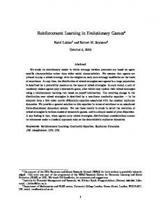
Figure 1: Penalty Game Results

Z

straightforward definition of the following terms: Pr(a−i |b)

=

Pr(t|a, b) = Pr(r|b) =

Z Z

σ−i

m

m

Pr(a−i |σ−i )PS (σ−i )

(5)

Pr(t|s, a, m)PM (m)

(6)

Pr(r|s, m)PM (m)

(7)

We note that the evaluation of Eqs. 6 and 7 is trivial using the decomposed Dirichlet priors mentioned above. This formulation determines the optimal policy as a function of the BA’s belief state. This policy incorporates the tradeoffs between exploration and exploitation, both with respect to the underlying (dynamics and reward) model, and with respect to the behavior of other agents. As with Bayesian RL and Bayesian learning in games, no explicit exploration actions are required. Of course, it is important to realize that this model may not converge to an optimal policy for the true underlying stochastic game. Priors that fail to reflect the true model, or unfortunate samples early on, can easily mislead an agent. But it is precisely this behavior that allows an agent to learn how to behave well without drastic penalty.

3.2 Computational Approximations Solving the belief state MDP above will generally be computationally infeasible. In specific MARL problems, the generality of such a solution—defining as it does a value for every possible belief state—is not needed anyway. Most belief states are not reachable given that an agent has a specific initial belief state. A more directed search-based solution technique can be used to solve this MDP for the agent’s current belief state b. We consider a form of myopic EVOI in which only immediate successor belief states are considered, and their optimal values are estimated without using VOI or lookahead. Formally, myopic action selection is defined as follows. Given belief state b, we define the myopic Q-function for each ai ∈ Ai as: Qm (ai , b) =

X

X

Pr(a−i |b)

a−i

Pr(t|ai ◦ a−i , b)

t

Pr(r|ai ◦ a−i , b)[r + γVm (b(hs, a, r, ti))]

r

Vm (b) = max ai

X

Z Z m

σ−i

(8)

Q(ai , s|m, σ−i )PM (m)PS (σ−i ) (9)

The action performed is that with maximum myopic Q-value. Eq. 8 differs from Eq. 3 in the use of the myopic value function Vm , which

is defined as the expected value of the optimal action at the current state, assuming a fixed distribution over models and strategies.8 Intuitively, this myopic approximation performs one step-lookahead in belief space, then evaluates these successor states by determining the expected value to BA w.r.t. a fixed distribution over models, and a fixed distribution over successor states. This computation involves the evaluation of a finite number of successor belief states—A · R · S such states, where A is the number of joint actions, R is the number of rewards, and S is the size of the state space (unless b restricts the number of reachable states, plausible strategies, etc.). It is important to note that more accurate results can be realized by doing multistage lookahead, with the requisite increase in computational cost. Conversely, the myopically optimal action can be approximated by sampling successor belief states (using the induced distributions defined in Eqs. 5, 6, 7) if the branching factor A · R · S is problematic. The final bottleneck involves the evaluation of the myopic value function Vm (b) over successor belief states. Note that the terms Q(ai , s|m, σ−i ) are Q-values for standard MDPs, and can be evaluated using standard methods, but direct evaluation of the integral over all models is generally impossible. However, sampling techniques can be used [5]. Specifically, some number of models can be sampled, the corresponding MDPs solved, and the expected Qvalues estimated by averaging over the sampled results. Various techniques for making this process more efficient can be used as well, including importance sampling (allowing results from one MDP to be used multiple times by reweighting) and “repair” of the solution for one MDP when solving a related MDP [5]. Furthermore, for certain classes of problems, such as repeated games, this evaluation can be performed directly. For instance, suppose a repeated game is being learned, and the BA’s strategy model consists of fictitious play beliefs. The immediate expected reward of any action ai taken by the BA (w.r.t. a specific successor belief state b0 ) is given by its expectation with respect to its estimated reward distribution and fictitious play beliefs. The maximizing action a∗i with highest immediate reward will be the best action at all subsequent stages of the repeated game—and has a fixed immediate reward r(a∗i ) under the myopic (value) assumption that beliefs are fixed by b0 . Thus the long-term value at b0 is given by r(a∗i )/(1−γ). The approaches above are motivated by approximating the direct myopic solution to the “exploration POMDP.” A different approach to this approximation is proposed in [5]. That algorithm does not We note that Vm (b) only provides a crude measure of the value of belief state b under this fixed uncertainty. Other measures could include the expected value of V (s|m, σ−i ). 8


a a; 0 s1

a a; 0

b b; 2

a a; 0 s3

s2 b b; 2

a a; 0

b b; 2

s4

s5

140


a a; 10


3.5

3

2.5

2

1.5

1

Bayesian Exploration WoLF

0.5

120

100

80


60

40

20

b b; 2 0

0 0

(a) Chain World Domain

5

10

15


35

40

(b) γ = 0.75

45

50

0

20

40

60


120

140

160

(c) γ = 0.99

Figure 2: Chain World Results

do one-step lookahead in belief space, but rather estimates the (myopic) value of obtaining perfect information about Q(a, s). Suppose that, given an agent’s current belief state, the expected value of action a is given by Q(a, s). Let a1 be the action with highest expected Q-value and state s and a2 be the second-highest. We define the gain associated with learning that the true value of Q(a, s) (for any a) is in fact q as follows:

method (BOL) and the naive sampling method for estimating VPI (BVPI) described in Section 3. In all cases, the Bayesian agents use a simple fictitious play model to represent their uncertainty over the other agent’s strategy. Thus at each iteration, a BA believes its opponent to play an action with the empirical probability observed in the past (for multistate games, these beliefs are independent at each state). BOL is used only for repeated games, since these allow the imQ(a2 , s) − q, if a = a1 and q < Q(a2 , s) mediate computation of expected values over the infinite horizon at gain s,a (q) = q − Q(a1 , s), if a 6= a1 and q > Q(a1 , s) the successor belief states: expected reward for each joint action can 0, otherwise readily be combined with the BA’s fictitious play beliefs to compute the expected value of an action (over the infinite horizon) since the Intuitively, the gain reflects the effect on decision quality of learning only model uncertainty is in the reward. BVPI is used for both rethe true Q-value of a specific action at state s. In the first two cases, peated and multi-state games. In all cases, five models are sampled what is learned causes us to change our decision (in the first case, to estimate the VPI of the agent’s actions. The strategy priors for the estimated optimal action is learned to be worse than predicted, the BAs are given by Dirichlet parameters (“prior counts”) of 0.1 or and in the second, some other action is learned to be better than pre1 for each opponent action. The model priors are similarly uninfordicted). In the third case, no change in decision at s induced, so the mative, with each state-action pair given the same prior distribution information has no impact on decision quality. Adapted to our setting, a computational approximation to this approach—over reward and transition distributions (except for one experiment as noted). called naive sampling in [5]—involves the following steps: We first compare our method to several different algorithms on a (a) a finite set of k models is sampled from the density PM ; stochastic version of the penalty game described above. The game is altered so that joint actions provide a stochastic reward, whose (b) each sampled MDP j is solved (w.r.t. the density PS over stratemean is the value shown in the game matrix.9 We compare the Bayesian j gies), giving optimal Q-values Q (ai , s) for each ai in that MDP, approach to the following algorithms. KK refers to the algorithm of and average Q-value Q(ai , s) (over all k MDPs); Kapetanakis and Kudenko [12] that biases exploration to encourage (c) for each ai , compute the gain w.r.t. each Qj (ai , s); define EVPI(ai , s) convergence to optimal equilibria in exactly these types of games. Two related heuristic algorithms that also bias exploration optimistito be the average (over the k MDPs) of gain s,ai (Qj (ai , s)); cally are the Optimistic Boltzmann (OB) and Combined OB (CB) [4] are also evaluated. Unlike KK, these algorithms observe and (d) define the value of ai to be Q(ai , s) + EVPI(ai , s) and execute make predictions about the other agent’s play. Finally, we test the the action with highest value. more general algorithm WoLF-PHC [3], which works with arbitrary, This approach can benefit from the use of importance sampling and general-sum stochastic games (and has no special heuristics for equirepair (with minor modifications). A key advantage of this approach librium selection). In each case the game is played by two learning is that it can be more computationally effective than one-step lookaagents of the same type. The parameters of all algorithms were emhead (which requires sampling and solving MDPs from multiple bepirically tuned to give good performance. lief states). The price paid is approximation inherent in the perfect The first set of experiments tested these agents on the stochastic information assumption: the execution of joint action a does not penalty game with k set to −20 and discount factors of 0.95 and come close to providing perfect information about Q(a, s). 0.75. Both BOL and BVPI agents use uninformative priors over the set of reward values.10 Results appear in in Figures 1(a) and (b) 4. EXPERIMENTAL RESULTS showing the total discounted reward accumulated by the learning agents, averaged over 30 trials. Discounted accumulated reward proWe have conducted a number of experiments with both repeated games and stochastic games to evaluate the Bayesian approach. We 9 focus on two-player identical interest games largely to compare to Each joint action gives rise to X distinct rewards. 10 existing methods for “encouraging” convergence to optimal equiSpecifically, any possible reward (for any joint action) is given libria. The Bayesian methods examined are the one-step lookahead equal (expected) probability in the agent’s Dirichlet priors.

8< :


6

200

**

+10

a,a; b,b s2 a,b; b,a a*

s5

**

-10

s1 b* **

s3

s6


s4


180 5

4

3

2


1

(a) The Opt In or Out Domain

140 120 100


80 60 40 20 0

+6 0

**

160

-20 0

5

10

15


35

40

45

50

(b) γ = 0.75

0

20

40

60


120

140

160

(c) γ = 0.99

Figure 3: “Opt In or Out” Results: Low Noise

vides a suitable way to measure both the cost being paid in the attempt to coordinate as well as the benefits of coordination (or lack thereof). The results show that both Bayesian methods perform significantly better in this regard than the methods designed to force convergence to an optimal equilibrium. Indeed, OB, CB and KK converge to an optimal equilibrium in virtually all of their 30 runs, but clearly pay a high price for this.11 By comparison, when γ = 0.95, the ratio of convergence to an optimal equilibrium, the nonoptimal equilibrium, or a nonequilibrium is, for BVPI 25/1/4 and for BOL 14/16/0. Surprisingly, WoLF-PHC does better than OB, CB and KK in both tests. In fact, this method outperforms the BVPI agent in the case of γ = 0.75 (this is due largely to the fact that the BVPI converges on a nonequilibrium 5 times and the suboptimal equilibrium 4 times). WoLF-PHC does converge in each instance to an optimal equilibrium. We repeated this comparison on a more “difficult” problem with a mean penalty of -100 (and increasing the variance of the reward for each action). To test one of the benefits of the Bayesian perspective we included a version of BOL and BVPI with informative priors (giving it strong information about the value of the rewards). Results are shown in Figure 1(c) (averaged over 30 runs). WolfPHC and CB converge to the optimal equilibrium each time, while the increased reward stochasticity made it impossible for KK and OB to converge at all. All four methods perform poorly w.r.t. discounted reward. The Bayesian methods perform much better. Not surprisingly, the agents BOL and BVPI with informative priors do better than their “uninformed” counterparts; however, because of the high penalty (despite the high discount factor), they converge to the suboptimal equilibrium most of the time (22 and 23 times, respectively). We also applied the Bayesian approach to two identical-interest, multi-state, stochastic games. The first is a version of Chain World [5] modified for multiagent coordination, and is illustrated in Figure 2(a). The optimal joint policy is for the agents to do action a at each state, though these actions have no payoff until state s5 is reached. Coordinating on b leads to an immediate, but smaller, payoff at each state, and resets the process.12 Unmatched actions ha, bi and hb, ai result in zero-reward self-transitions (omitted from the diagram for clarity). Transitions are noisy, with a 10% chance that an agent’s action has the “effect” of the opposite action. The original Chain World is difficult for standard RL algorithms, and is made 11

All penalty game experiments were run to 500 games, though only the interesting initial segments of the graphs are shown. 12 As above, rewards are stochastic with means shown in the figure.

especially difficult here by the requirement of coordination to make progress. We compared BVPI to WoLF-PHC on this domain using two different discount factors, plotting the total discounted reward received (averaged over 30 runs) in Figure 2(b) and (c). These graphs show the initial segments only, though the results project smoothly to 50000 iterations. We see that BVPI compares favorably to Wolf-PHC in terms of online performance. The Bayesian agents converged to the optimal policy in 7 (of 30) runs with γ = 0.99 and in 3 runs with γ = 0.75, intuitively reflecting the increased risk aversion due to increased discounting. WoLF-PHC rarely even managed to reach state s5 , though in 2 (of 30) runs with γ = 0.75 it stumbled across s5 early enough to converge to the optimal policy. The Bayesian approach in this case manages to encourage intelligent exploration of action space in a way that trades off risks and predicted rewards; and we see increased exploration with the higher discount factor, as expected. The second multi-state game is “Opt in or Out” game shown in Figure 3(a). The transitions are stochastic, with the action selected by an agent having the “effect” of the opposite action with some probability. Two versions of the problem were tested, one with low “noise” (probability 0.05 of an action effect being reversed), and one with “medium” noise level (probability roughly 0.11). With low noise, the optimal policy is as if the domain were deterministic (the first agent opts in at s1 and both play a coordinated choice at s2 ), while with medium noise, the “opt in” policy and the “opt out” policy (where the safe play of moving to s6 is adopted) have roughly equal value. BVPI is compared to WoLF-PHC under two different discount rates, with low noise results shown in Figure 3(b) and (c), and high noise results in Figure 4(a) and (b). Again in terms of discounted reward, the Bayesian agents compare favorably to WoLFPHC. In the low noise problem, BVPI converged to the optimal policy in 18 (of 30) runs with γ = 0.99 and 15 runs with γ = 0.75. The WoLF agents converged in the optimal policy only once with γ = 0.99, but 17 times with γ = 0.75. With medium noise, BVPI chose the “opt in” policy in 10 (0.99) and 13 (0.75) runs, but did manage to learn to coordinate at s2 even in the “opt out” cases. Interestingly, WoLF-PHC always converged on the “opt out” policy (recall both policies are optimal with medium noise).

5. CONCLUDING REMARKS We have described a Bayesian approach to the modeling of MARL problems that allows agents to explicitly reason about their uncertainty regarding the underlying domain and the strategies of their counterparts. We’ve provided a formulation of optimal exploration


4.5


4 3.5 3


2.5 2 1.5 1 0.5 0 -0.5 0

5

10

15


35

40

45

50

(a) γ = 0.75 Discounted Average Accumulated Reward (over 30 runs)

160

140

120

100


80

60

40

20

0

-20 0

20

40

60


120

140

160

(b) γ = 0.99 Figure 4: “Opt In or Out” Results: Medium Noise

under this model and developed several computational approximations for Bayesian exploration in MARL. The experimental results presented here demonstrate quite effectively that Bayesian exploration enables agents to make the tradeoffs described. Our results show that this can enhance online performance (measured as reward accumulated while learning) of MARL agents in coordination problems, when compared to heuristic exploration techniques that explicitly try to induce convergence to optimal equilibria. This implies that BAs run the risk of converging on a suboptimal policy; but this risk is taken “willingly” through due consideration of the learning process given the agent’s current beliefs about the domain. Still we see that BAs often find optimal strategies in any case. Key to this is a BA’s willingness to exploit what it knows before it is very confident in this knowledge—it simply needs to be confident enough to be willing to sacrifice certain alternatives. While the framework is general, our experiments were confined to identical interest games and the use of fictitious play-style beliefs as (admittedly simple) opponent models. These results are encouraging but need to be extended in several ways. Empirically, the application of this framework to more general problems is of critical importance to verify its utility. More work on computational approximations to estimating VPI or solving the belief state MDP is also needed. Finally, the development of computationally tractable means of representing and reasoning with distributions over strategy models is required.

6.

REFERENCES

[1] C. Boutilier. Sequential optimality and coordination in multiagent systems. In Proceedings of the Sixteenth International Joint Conference on Artificial Intelligence, pages 478–485, Stockholm, 1999.

[2] M. Bowling. Convergence problems of general-sum multiagent reinforcement learning. In Proceedings of the Seventeenth International Conference on Machine Learning, pages 89–94, Stanford, CA, 2000. [3] M. Bowling and M. Veloso. Rational and convergent learning in stochastic games. In Proceedings of the Seventeenth International Joint Conference on Artificial Intelligence, pages 1021–1026, Seattle, 2001. [4] C. Claus and C. Boutilier. The dynamics of reinforcement learning in cooperative multiagent systems. In Proceedings of the Fifteenth National Conference on Artificial Intelligence, pages 746–752, Madison, WI, 1998. [5] R. Dearden, N. Friedman, and D. Andre. Model-based bayesian exploration. In Proceedings of the Fifteenth Conference on Uncertainty in Artificial Intelligence, pages 150–159, Stockholm, 1999. [6] J. A. Filar and K. Vrieze. Competitive Markov Decision Processes. Springer Verlag, New York, 1996. [7] Drew Fudenberg and David K. Levine. The Theory of Learning in Games. MIT Press, Cambridge, MA, 1998. [8] J. C. Harsanyi and R. Selten. A General Theory of Equilibrium Selection in Games. MIT Press, Cambridge, 1988. [9] J. Hu and M. P. Wellman. Multiagent reinforcement learning: Theoretical framework and an algorithm. In Proceedings of the Fifteenth International Conference on Machine Learning, pages 242–250, Madison, WI, 1998. [10] P. Jehiel and D. Samet. Learning to play games in extensive form by valuation. NAJ Economics, Peer Reviews of Economics Publications, 3, 2001. [11] E. Kalai and E. Lehrer. Rational learning leads to Nash equilibrium. Econometrica, 61(5):1019–1045, 1993. [12] S. Kapetanakis and D. Kudenko. Reinforcement learning of coordination in cooperative multi-agent systems. In Proceedings of the Eighteenth National Conference on Artificial Intelligence, pages 326–331, Edmonton, 2002. [13] M. Lauer and M. Riedmiller. An algorithm for distributed reinforcement learning in cooperative multi-agent systems. In Proceedings of the Seventeenth International Conference on Machine Learning, pages 535–542, Stanford, CA, 2000. [14] M. L. Littman. Markov games as a framework for multi-agent reinforcement learning. In Proceedings of the Eleventh International Conference on Machine Learning, pages 157–163, New Brunswick, NJ, 1994. [15] M. L. Littman and C. Szepesv´ari. A generalized reinforcement-learning model: Convergence and applications. In Proceedings of the Thirteenth International Conference on Machine Learning, pages 310–318, Bari, Italy, 1996. [16] J. Robinson. An iterative method of solving a game. Annals of Mathematics, 54:296–301, 1951. [17] L. S. Shapley. Stochastic games. Proceedings of the National Academy of Sciences, 39:327–332, 1953. [18] M. Tan. Multi-agent reinforcement learning: Independent vs. cooperative agents. In Proceedings of the Tenth International Conference on Machine Learning, pages 330–337, Amherst, MA, 1993. [19] X. Wang and T. Sandholm. Reinforcement learning to play an optimal nash equilibrium in team markov games. In Advances in Neural Information Processing Systems 15 (NIPS-2002), Vancouver, 2002. to appear.