Correct Small-Truncated Excited State Wave functions Obtained via Minimization Principle for Excited States compared / opposed to Hylleraas-Undheim and McDonald higher “roots” Z. Xiong1,2, b), J. Zang1, H.J. Liu1, D. Karaoulanis3, Q. Zhou2 and N.C. Bacalis4, a) 1
Space Science and Technology Research Institute, Southeast University, Nanjing, 21006, Peoples Republic of China 2 School of Economics and Management, Southeast University, Nanjing 210096, Peoples Republic of China 3 Korai 21, Halandri, GR-15233, Greece. 4 Theoretical and Physical Chemistry Institute, National Hellenic Research Foundation, Athens, GR-11635, Greece a)
Corresponding author:
[email protected] b)
[email protected]
Abstract. We demonstrate that, if a truncated expansion of a wave function is large, then the standard excited states computational method, of optimizing one “root” of a secular equation, according to the theorem of Hylleraas, Undheim and McDonald (HUM), tends to the correct excited wave function, comparable to that obtained via our proposed minimization principle for excited states [J. Comput. Meth. Sci. Eng. 8, 277 (2008)] (independent of orthogonality to lower lying approximants). However, if a truncated expansion of a wave function is small - that would be desirable for large systems - then the HUM-based methods may lead to an incorrect wave function - despite the correct energy (: according to the HUM theorem) whereas our method leads to correct, reliable, albeit small truncated wave functions. The demonstration is done in He excited states, using truncated series “small” expansions both in Hylleraas coordinates, and via standard configuration-interaction truncated “small” expansions, in comparison with corresponding “large” expansions. Beyond that, we give some examples of linear combinations of Hamiltonian eigenfunctions that have the energy of the 1st excited state, albeit they are orthogonal to it, demonstrating that the correct energy is not a criterion of correctness of the wave function.
Introduction In ab-initio computations of the properties of any system the wave functions are necessarily truncated. Large wave function expansions in truncated - but as complete as possible - Hilbert spaces, are generally safe, but if the system is large, the large wave functions are rather impracticable. Thus, small and handy, but reliable, expansions are much preferable, provided that they curry the main properties of the system, leaving the improvement of the energy to any correlation-corrections (by describing the “splitting” of the wave function in areas of accumulated electrons). For the ground state, such a “useful” wave function is relatively easily obtained by minimizing the energy, but for excited states, minimization of the energy can only be achieved if the wave function is orthogonal to all lower states. However, this requires accurate large expansions; otherwise, orthogonality to inaccurate approximations of lower states must lead to an energy lying below the exact (without collapsing to lower states) [1]. On the other hand, if the calculation of the ground state and excited states are optimized by variation respectively, such as the State-Specific Theory [2], based on approximated orthogonality, the energy of the ground state and the excited states can be obtained with good accuracy, but the orthogonality between the whole ground and excited state wave functions will be destroyed, and thus can not guarantee the
accuracy of the approximate wave function. Particularly, this would render the calculation of properties between different states (e.g., optical transitions, the oscillator strength, etc.) unable to guarantee its reliability. This is why the spectral line positions of atoms and ions, obtained by many experiments and astronomical observations can be accurately theoretically explained, but their intensity distribution is difficult to be obtained with satisfactory theoretical description. Here we compute both “large” and “small” wave functions of ground and excited states of He (the smallest non-trivial system) using two methods, the standard method based on the theorem of Hylleraas, Undheim and McDonald (HUM) [3] of optimizing desired “roots” of a secular equation, and our method, based on our proposed minimization principle for excited states (VPES, “F”) [1], which - it is important to mention - does not use any orthogonality to lower-lying approximate wave functions. This allows approaching the exact Hamiltonian eigenfunction, even in small truncated spaces. For demonstration purposes we use two kinds of wave function expansions, i.e. (i) series expansions in Hylleraas coordinates [3] (the most accurate for He atom) and (ii) configuration interaction (CI) expansions in standard spatial coordinates [1]. First we demonstrate that if the expansion is large enough, then - as expected for large expansions - the standard methods based on HUM, and our method, “F”, give practically identical wave functions, confirming that our method is valid and reliable. Further, considering the traditional standard method of orthogonalizing to all truncated wave functions lying lower than the desired excited one, we demonstrate that if the functions are “small” - i.e., if, in optimizing the desired root of the (small) secular equation, the optimized small excited function is orthogonal to the lower roots that are small functions then, in spite of the fact that the energy may converge from above to the correct value according to the theorem of Hylleraas, Undheim and McDonald (HUM) [3], the imposed orthogonality (i.e. to truncated approximants) may lead to disastrously incorrect main orbitals which are unable to describe the main properties, and indispensably need correlation orbitals that try to “improve” the total wave function (not the main orbitals), thus prohibiting a correct identification of the main orbitals, e.g. as to a correct “HOMO” or “LUMO”. On the contrary, minimization of our proposed functional F [1], leads to a correct (small) wave function, which curries the same main properties as the “large” function (obtained comparable, and safely, by either HUM or F). As an example, in He 3S 1s3s, HUM “small” leads to 1s2s+correlation corrections (instead of 1s3s), whereas our “F” “small” leads to the correct 1s3s. It is important to note that F has a local minimum at the excited state, therefore, it does not need any orthogonalization to lower lying wave functions, it just insures solution of the Schrödinger equation; orthogonality to exact lower states should be an outcome. The demonstration is done in He excited states, using truncated series expansions in Hylleraas coordinates, as well as standard configuration-interaction (CI) truncated expansions in comparison with corresponding “large” expansions. In the following, after a brief discussion about the saddleness of the excited state energy, we present: (1) Our tools and approximations; (2) Our methods; (3) We demonstrate: (i) The validity and reliability of our method by showing the equivalence of “large” expansions obtained either via HUM or via F, i.e. by displaying the main orbitals, as well as average values of r n , n=-1,0,1,2; And: (ii) That “small” expansions obtained via F are correct (with main orbitals comparable to those of “large” functions) whereas those obtained via HUM may give misleadingly incorrect
main orbitals, with concomitant incorrect practical conclusions as to which HUM orbitals are HOMO/LUMO, or as to which HUM orbitals contribute to charge transfer. (4) Then, since the excited states are saddle points [cf. below], and around a saddle point some actual computation, like minimizing “F”, may stop, to within a convergence criterion, at the side with energy of either E+∆Ε or E–∆Ε, we state three reliability criteria in case that the minimization converges at the side of energy just below the saddle point energy of the correct excited state, i.e. at E–∆Ε - a subject which is never encountered by any standard method based on HUM because HUM always converges from above (to a function [cf. function “ΦHUM” in Fig. 1] which is necessarily veered away from the exact eigenfunction [cf. function “ψ1” in Fig. 1]). (5) Finally we give some examples of truncated wave functions that have exactly the energy of an excited state, but are orthogonal to it(!), demonstrating that the correct energy is not a safe criterion of the correctness of the wave function. The saddleness of the excited state energy En Expand the approximant φn around the exact state n (assumed real, non-degenerate, and normalized) in terms of the exact Hamiltonian eigenfunctions i , i=0,1,...n,..., with energies E0 < E1 < E2 "
φn =
∑
in
(1)
i i φn
The energy is written as φn H φn = E = − L + En + U where, in terms of the coefficients, the lower terms, L, and the higher terms, U, (saddle) are: down - paraboloids and up - paraboloids : E = −L = −
∑
in
( Ei − En )
i φn
2
(2)
If L is absent, i.e. if n=0 (Eckart theorem [4]), or if φn is orthogonal to all lower ψ = i (which can be approximated by φi satisfactorily only if φi are “large” expansions), then minimizing E=En+U is sufficient. But if φi are “small” expansions (not accidentally orthogonal to φn), then L is present, and E has a saddle point at n . Then, minimizing E=L+En+U “orthogonally to all lower approximants φi”, must lead to E below En; because (consider e.g. the 1st excited state): If φ0 is such an (inaccurate) approximant of ψ0, i.e. if φ0 is not orthogonal to ψ1, then in the subspace orthogonal to φ0, there is a function φ1+, which is: “closest to ψ1 (while orthogonal to φ0)”. Closest to ψ1 means it has no other components out of the plane of {φ0, ψ1}. It is easily seen that this function, φ1+, lies below E1 (therefore, the minimum lies even lower): i
φ1 ≡ (ψ 1 − φ0 ψ 1 φ0 +
φ1 H φ1 +
+
)/
1 − ψ 1 φ0
2
⇒
= E ⎡⎣φ1 ⎤⎦ = E [ψ 1 ] − ( E [ψ 1 ] − E [φ0 ]) ψ 1 φ0 +
2
(
/ 1 − ψ 1 φ0
2
)⇒
(3)
E ⎡⎣φ1 ⎤⎦ < E [ψ 1 ] = E1 +
But the HUM theorem demands E[φn] > En while φn is orthogonal to all lower “roots” φi of the secular equation. Therefore, on the subspace orthogonal to the lowest root, the function which is closest to ψ1, while orthogonal to the lowest root, i.e. φ1+, is not accessible by HUM (and even more inaccessible is ψ1 itself). Even worse, note that in optimizing any HUM root (say 2
φ1), all other roots (φ0,φ2, ...) get deteriorated since we may have 1 φ1 → 1, at will , but :
0 φ0
2
+ 0 φ1
2
+ 0 φ2
2
This means that, if 1 φ1
+ " + 0 φN 2
2
≤ 1 ⇒ 0 φ0
2
< 1 − 0 φ1
2
(: accuracy upper bound )
(4)
2
approaches → 1, at will , then 0 φ0 cannot approach → 1, at will ,
φ0 having to be deteriorated (of worse quality than φ1), especially if it is “small” because then, 2 2 1 φ1 < 1, 0 φ1 < 1 .
Fig. 1. Schematic representation of states. All states are assumed normalized: ψ0, ψ1, ψ2, ... with energies E0< E1< E2< ... are the unknown exact eigenstates; φ0 is a known approximant of ψ0 (not orthogonal to ψ1). The subspace orthogonal to φ0, is S = {Φ, φ1+} (oblique circle orthogonal to the vertical circle of {φ0, ψ1} and orthogonal to φ0), and if φ0 is not (accidentally) orthogonal to the unknown ψ1, then S = {Φ, φ1+} does not contain ψ1. In the subspace S = {Φ, φ1+}, the closest approximant to ψ1 is φ1+ (the intersection of the oblique circle and the vertical circle of { φ0, ψ1}), and, as explained in the text, φ1+ lies below ψ1: E[φ1+] < E1. In going, in S, orthogonally to φ0, from φ1+ toward a state near ψ2 (the diameter of the oblique circle near ψ2), i.e. in going, in S, from E[φ1+] < E1 toward E ≈ E2 > E1, one passes from E1, i.e. from states, φ1, of S, orthogonal to φ0, but having energy E[φ1] = E1. If, in optimizing φ1 by HUM theorem, φ0 is the lowest (deteriorated, as explained in the text) root of the secular equation, then the 2nd “root”, φ1 = ΦHUM, is one of these states, “φ1”, with lowest possible (allowed by HUM theorem) energy E[φ1] = E[ΦHUM] = E1 (cf. left “minimum” in the figure on the oblique circle S). But, evidently, φ1 = ΦHUM is not ψ1. It might be desirable to continue optimization in S toward, at least, φ1+, the closest, in S, to ψ1. But HUM theorem prohibits such a continuation, since the 2nd root must always be higher than E1. In an attempt to approach, as much as possible, ψ1, one might try, by other means, i.e. by direct minimization, to minimize the energy, in S, orthogonally to φ0, toward φ1+. But φ1+ is not a critical point, and the minimum in S, orthogonal to φ0, lies even lower: E[ΦMin] E1 > E[φ1+]) is orthogonal to a deteriorated 1st root φ0, which, consequently, has a deteriorated φ1+ (the “closest to ψ1 while orthogonal to the deteriorated φ0”) (cf. Fig. 1); i.e. φ1, moving in space orthogonal to deteriorated φ0s, just stops at E1 and cannot approach a deteriorated φ1+, thus, the optimized HUM 2nd root φ1 is much more veered away from the exact ψ1. This is clearly demonstrated below for He. (If the optimized wave functions, as HUM roots, are misleading even for the smallest atom, He, then there is no guarantee for the correctness of HUM roots in larger systems!)
Tools and approximations First we need very accurate (truncated) functions Ψn to resemble> eigenfunctions ψn as well as truncated approximants Φn to check the closeness to ψn i.e. to Ψn. As truncated functions we use: 1. For He 1S (1s2 and
1s2s):
G G s = r1 + r2 , t = r1 − r2 , u = r1 − r2 .
Series
expansion
in
Hylleraas
variables
The two-electron wave function Φ(r1,r2) consist of one Slater determinant of variational Laguerre–type orbitals (VLTOs), 1s, 2s χ ( n, r ; z n ,{an , k }) =
4 π
( n − 1)! n ! n
2
n −1
3/ 2
zn
k
∑ k =0
an , k ( −2 rz n / n ) e
− rz n / n
k !( k + 1)!( n − k − 1)!
(5)
(where r1 = ( s + t ) / 2, r2 = ( s − t ) / 2 and an , k , zn are free variational parameters), and where the determinant is multiplied by a truncated power series of s,t,u: Φ(r1,r2) = Det χ1 , χ 2 ×
ns , nt , nu
∑
is ,it ,iu = 0
cis ,it ,iu s is t 2it u iu ,
(6)
where c’s are linear variational parameters, comprising the eigenvectors of the 1st or 2nd root of a secular equation. For the “exact” Ψn we take terms up to (ns,nt,nu) = (2,2,2): 27 terms, E0 ≈ -2.90371 a.u., E1 ≈ -2.14584 a.u., compared to Pekeris’ 95 terms: E0= -2.90372, E1= -2.14597 a.u. [5]. For the “truncated” trial “small” functions Φn we take terms up to (ns,nt,nu) = (1,1,1): 8 terms. 2. For He 1S (1s2, 1s2s and 1s3s) and for He 3S (1s2s and 1s3s) we use Configuration Interaction (CI) in standard spherical coordinates (r,θ,φ). In this approximation the two-electron wave function Φ(r1,r2) is a linear combination of configurations composed of Slater determinants (SD) of atomic variationally optimized Laguerre-type (VLTO) spin-orbitals, which have been proven [6] to provide conciseness, clear physical interpretation and near equivalent accuracy with numerical multi-configuration self-consistent field (MCHF) - which is one of the most accurate numerical methods for atomic CI calculations. The VLTO atomic orbitals are orthogonalized by appropriate g kn ,A factors: r r n − A −1 − zn , A − q n , A zn , A ⎞ n ,A ,m ⎛ n ,A n ,A ( A + k ) n ,A n n +b e A e δ A ,0 ⎟ Y A ,m (θ , φ ) (7) ⎜ ∑ ck g k r ⎝ k =0 ⎠ where, variational parameters are: the quantities zn,ℓ, bn,ℓ, qn,ℓ, along with the linear CI coefficients as eigenvectors of the roots of the secular equation. As “exact” Ψn we use a “large” expansion in 1s, 2s, 3s, 4s, 5s, 2p, 3p, 4p, 5p, 3d, 4d, 5d, 4f, 5f. For 1S: E0 ≈ -2.90324 a.u., E1 ≈ -2.14594 a.u., E2 ≈ -2.06125 a.u. (exact: -2.06127 a.u. [5]), for 3S: E0 ≈ -2.17521 a.u., E1 ≈ -2.06869 a.u. (exact: -2.17536, -2.06881 a.u. [5]). (The ground state is slightly harder to converge: it needs more configurations near the nucleus.) As “truncated” trial functions Φn we use a “small” expansion in 1s, 2s, 3s. The two methods used In both of the above approximations we shall use two methods: 1. Minimimizing (optimizing) directly the nth HUM root, which, as aforementioned, must be veered away from the exact eigenfunction ψn (because, according to the HUM theorem it tends to the exact energy from above, i.e. it cannot go to lower energies, required
in order to approach closer the exact ψn, due to orthogonality to lower roots which are deteriorated). 2. Minimimizing the functional Fn that has minimum at the exact ψn [1] Fn ⎣⎡φ0 , φ1 ,...; φn ⎦⎤ ≡ E[φn ] + 2
∑ i