Mar 6, 2008 - In particular, we consider Calderbank-Shor-Steane codes and observe a better .... where the âmap operatorsâ {Fα} are v à u matrices and the.
Correlated errors can lead to better performance of quantum codes A. Shabani1 1
Department of Electrical Engineering, University of Southern California, Los Angeles, California 90089, USA A formulation for evaluating the performance of quantum error correcting codes for a general error model is presented. In this formulation, the correlation between errors is quantified by a Hamiltonian description of the noise process. We classify correlated errors using the system-bath interaction: local versus nonlocal and two-body versus many-body interactions. In particular, we consider Calderbank-Shor-Steane codes and observe a better performance in the presence of correlated errors depending on the timing of the error recovery. We also find this timing to be an important factor in the design of a coding system for achieving higher fidelities.
arXiv:quant-ph/0703142v2 6 Mar 2008
PACS numbers: 03.67.Pp, 03.67.Hk, 03.67.Lx
I. INTRODUCTION
The theory of fault-tolerant quantum computation (FTQC) has been developed as a realistic extension of the ideal theory of quantum computation. In an ideal prototype, all computational components are functioning with no deficiency, while in the real world deviations from the ideal design is inevitable. This can be due to imperfections in the components or interactions imposed by the environment. In FTQC, schemes of error correction are combined with computational elements in a special design to prevent the spread of errors through a circuit. Applying error correction steps in a multi-layer circuit is a well established procedure for FTQC [1, 2, 3, 4, 5, 6, 7]. Inspired by classical coding theory, a fault-tolerant form of quantum error correction codes (QECCs) can be achieved by concatenating single units of encoding. The performance of fault-tolerant codes has been studied for various noise models. The classical model of a Markovian-independent noise has been thoroughly investigated in the literature [1, 2, 3, 4]. In this picture, each individual component of the circuit is only coupled to a single designated bath, with no cross talk between the baths. In addition, each bath is assumed to be large enough to constitute a local Markovian decoherence channel. Other possible defects coming from imperfections in computational gates are also assumed to have local and instantaneous effects. All these give rise to a probabilistic description of the noise process. Upper bounding the error probability guarantees an arbitrary small likelihood of computational failure. However, an analysis of quantum computer proposals reveals the inaccuracy of the above noise model. For example, ion qubits in an ion trap setup are collectively coupled to their vibrational modes [9]. In a quantum dot design, different qubits are coupled to the same lattice, thus interacting with a common phonon bath [10]. The exchange interaction is the main candidate for implementing two-qubit gates in solidstate proposals. Recently, it has been shown that many-body exchange interactions can be strong enough to act as a major source of noise [11]. Equally important, collective control of the qubits may also give rise to errors due to the inaccuracy of the control field [12]. These examples invalidate the assumption of error independence (locality in space). In addition, the non-Markovian nature of noise has been observed in various
systems [13]. Therefore, the assumptions of exact locality in time and space should be relaxed to attain a more realistic model [14]. First attempts to introduce correlations into noise models were in a classical manner: multilocation joint probabilities that are stronger than the independent model [1, 3]. Recently a physical approach to the problem was taken by introducing a Hamiltonian description of the noise process[6, 7]. However, because of the discrete nature of error correction, the noise Hamiltonian was perturbatively treated to achieve a faulty paths description of the noisy computation. In another recent paper [8],the authors explicitly show the importance of a non-perturbative calculation of the FTQC threshold. In this paper, we study the performance of quantum codes in a single block of error correction towards a comprehensive analysis of the FTQC problem with a realistic model. Our aim is to compare spatial correlations in noise without any limiting assumptions on time. Focusing on well-defined CalderbankShor-Steane (CSS) codes [15], we first formulate a measure for the code performance and then apply it to different decoherence scenarios. Our main finding is that a coding system can function better in the presence of error correlations. This is mainly due to the entangling power of a common bath which can help in the preservation of the code-state coherence designated for recovery [16]. This is in contrast to results from previous studies [17, 18, 19, 20]. II. CORRELATED ERRORS
First we define the notion of correlation in errors. From the physical point of view, the primary probabilistic description of the noise originates from two main assumptions on the system-bath interaction: each qubit is coupled to its own bath, and the resulting decoherence is described by a completely positive (CP) map. A CP-map modeling of the noise process allows a probabilistic interpretation of the errors which may be otherwise impossible [21]. Based on this classical randomness picture, correlations could be defined by some joint probability distribution for the multi-qubit error operators. However, a microscopic description is lacking in such a model, motivating a more physical formulation. We remark that the source of error is either a second system with a large Hilbert
2 space or an imperfect driving field of a quantum gate. In general there are three possible scenarios as depicted in Fig. 1: (i) errors with no correlation, which corresponds to model of separated baths, each coupled only to a single qubit; (ii) short-range correlations in which all the qubits are only coupled to a common bath; and (iii) The most general case with long-range correlations where qubits are interacting with each other while sharing a common environment. In the following, we locate the qubits of a code in the above scenarios and compare their performance as a function of decoherence time τd . This is when we enter the recovery phase. The choice of CSS code is made to obtain an analytical solution to the problem. A [n, k, d] CSS code is an n−qubit code, encoding k bits of information, capable of correcting errors acting on at most t = [ d−1 2 ] different qubits. Consider an nqubit quantum code in a single step of error correction. The n qubits are sent through a noise channelP N expressed as a † completely positive (CP) map: N (ρS ) = α Eα ρS Eα . We 1 expand this map in the basis {Σα1 ,...,αn = σα1 ⊗ ... ⊗ σαnn }, N (ρS ) =
X
e{p},{q} Σ{p} ρS Σ{q}
�
(pi + qi ) has w nonzero elements, otherwise. (2) The noise map N (ρS ) can be decomposed as a sum of submaps Nw N (ρS ) =
e{p},{q} 0
X w
Nw (ρS ) =
X
ew {p},{q} Σ{p} ρS Σ{q}
w,{p},{q}
Qubit Coupling
(b)
(c)
Figure 1: A sketch of (a) an uncorrelated error model, (b) a shortrange correlation, and (c) a long-range correlation.
Theorem 1 Consider a CP noise map ΦCP (ρ) = P † F ρF and a code space P . A recovery CP map α C α α R correcting P the map ΦCP (ρ) can also correct a Hermitian map Φ(ρ) = α cα Fα ρFα† . Proof. This is a straightforward application of theorem 1 in Ref. [24]. It is obvious that the correctable sum noise map Nc is a Hermitian linear map by definition. Therefore one can find a recovery map R(ρ) inverting Nc , which belongs to the correctibility domain of a [n, k, d] code,; i.e. there exists a real number pN such that R ◦ N c = pN I.
(5)
where I is the identity superoperator.
(3)
We can separate the correctable (by means of a [n, k, d] CSS code) and uncorrectable parts of the P map by splitting the noise map into submaps N (ρ ) = c S w6t Nw (ρS ) and P Nic (ρS ) = td {p},{p} or e{p}6={q} which are of the order of 2 have verified this fact for a general noise model, justifying the bipartitioning of the noise map in Eq. (4). As a consequence, the fidelity average converges to a simple form of pN = Fave (|CihC|, R(N (|CihC|))) =
Different Size Baths Same Size Baths
0.2
ρS + (error).
By � of the performance measure, pN indp is equal P definition to tc=0 nc (1 − p)(1−c) pc . This value can be interpreted in the language of probability as the likelihood of having fewer than t individual errors [22]. In the above definition we discarded R ◦ N ic as the error. Actually this term vanishes in an averaging procedure introduced in Ref. [17]. Consider a code word ρS = |ΨihΨ| experiencing the noise N (ρS ) and being corrected by a CSS code recovery map R(ρ) =
0.4
N=196 Fidelity Difference
=
t X
N=7 Fidelity Difference
errors in up to t different locations in the code; then we have
X
en{p},{p} . (9)
n6t,{p}
Such a code-independent measure equips us with a quantitative tool to compare different noise models. Suppose system and bath start from an initial product state ρSB (0) P = ρS (0) ⊗ ρB (0), with the bath density matrix ρB (0) = i λi |bi ihbi |. For a system-bath propagator Uτd (τd is decoherence time before recovery operation), the√dynamical Kraus operators {Ei,j } can be written as Ei,j = λi hbj |Uτd |bi i. Now we can
pN (τd ) =
1 X Tr[TrS (Uτ†d Σ{υ} )TrS (Σ{υ} Uτd )ρB (0)]. 22n |υ|≤t
(10) In the following we apply this measure on different systembath interaction configurations.
IV. LOCAL vs NONLOCAL ENVIRONMENTS
Here we compare system-bath configurations (a) and (b) in Fig. 1: Each qubit is coupled to its own bath versus all qubits coupled to the same bath. We consider a spin star model which consists of a central spin- 21 particle representing a qubit, surrounded by N localized spin- 21 particles acting as a spin bath for the qubit [23]. In the local model the central spin σ is coupled to the bath spins σi , (i = 1, ..., N ) via a dephasing interaction of the form Hhf =
N X
gi σz Zi ,
(11)
i=1
where σz and Zi are the z components of σ and σi respectively. This is the effective Hamiltonian of dephasing in NMR due to spin-spin interactions [25]. Also this hyperfine contact type of interaction is a source of electron spin decoherence in quantum dots due to the interaction with nuclei [26]. In the presence of a strong magnetic field along the z direction, the
4
V. TWO-BODY vs MANY-BODY INTERACTIONS
We now introduce many-body interactions as a counterpart to multivariate joint probability in classical descriptions of correlations. In a recent study [7], the fault-tolerant quantum computation in the presence of many body interactions has been investigated. Following their formulation, we include additional terms Hij which act simultaneously on qubit pairs < ij > and on the bath. As an example consider the noise Hamiltonian
Hthree−body = g
N n X X j=1 i=1
σzj Zi + g ′
n X N X
σzj σzk Zi , (12)
j,k=1 i=1
in which g and g ′ determines the strength of two-body and three-body interactions. The ratio g ′ /g, in some specific configurations of spin- 21 particles, can rise up to 16% [11]. We compare two cases of two-body only interactions, with g ′ = 0, and three-body interactions with g ′ = 0.1g. As shown in
1.2 2−body 3−body
1
p3−body−p2−body 0.8
Fidelity
dephasing interaction is the dominant term in the hyperfine interaction [27]. Two different configurations of local and nonlocal decoherence for anP n-qubit PN code marem modn and eled as Hlocal = i=1 gim σz Zi m=1 Pn PN m Hnonlocal = As an example m=1 i=1 gim σz Zi . we consider a [7, 1, 3] code surrounded by N = {7, 196} bath spins [23]. The bath state, ρB in Eq.(10), is a thermal state of the spin bath at temperature PN T = 1mK with an internal Hamiltonian HB = i=1 ΩZi . In addition, for simplicity we assume a symmetric coupling gim = g. The difference of the performance of local and nonlocal models plocal (gτd ) − pnonlocal (gτd ) is plotted in Fig. 2. We observe N N that the performance strongly depends on the decoherence time τd . Consequently, choosing the correct time for recovery can improve the functioning of the code in the presence of correlations. This is in contrast to a classical system in which a common source of error acts simultaneously on different parts, and therefore leads to a higher risk of computational failure, while in the quantum case, indirect coupling of the qubits through a shared common bath or direct coupling by means of many-body interactions imposes additional dynamics on the code coherence that changes the performance of the code. Furthermore, these results reveal that engineering the qubits of a code block in the same location (non-local bath) may have an advantage over spatially separating them (local bath), as suggested in [7]. Another interesting comparison can be made between local and nonlocal baths of the same size, with the correspondPn PN/n m m ing Hamiltonians Hlocal = m=1 i=1 gim σz Zi and Pn PN m Hnonlocal = m=1 i=1 gim σz Zi . The simulation results are plotted in Fig. 2 which demonstrates the time-dependent, alternative behavior of the code performance difference.
0.6 0.4 0.2 0 −0.2 0
0.2
0.4
0.6
0.8
1
gτ
1.2
1.4
1.6
1.8
2
d
Figure 3: A [7,1,3] code performance in the presence of twobody and three-body interactions. The performance difference two−body pN (τd )−pthree−body (τd ) determines how the effect of threeN body interaction varies by decoherence time τd (N = 7).
Fig. 3, for short recovery times they behave similarly, while at longer times an alternative performance of two cases emerges. VI. FAULTY GATE
A faulty gate is another main source of errors in computation. In many proposals for quantum computers, a magnetic field or laser pulse is an ingredient of the control field which can act locally [22] or globally (nonlocally) [12]. Obviously an inaccuracy in manipulating the control field causes inaccuracy in the computation. Here we compare the fault tolerability of an n-qubit code driven P by an imperfect magn netic field acting locally (H = g ml i=1 Bi Zi ) or globPn ally (Hmg = gB0 i=1 Zi ). Because of the classical nature of the error, we assume a random process for the control error, i.e. Bi = Bideal + Wi , where the random variable Wi has a probability distribution pWi (w) = p(w). For a time τr the total rotation generated by this field is Pn Uml (w, τr ) = exp[−iτr g i=1 Bi (w)Z Pi ]nfor local control, and Umg (w, τr ) = exp[−iτr gB0 (w) i=1 Zi ] for global control. The distance of two unitary operations U and V , acting on a Hilbert space H, can be measured by the average fidelity Ave|ψi∈H hψ|V † U |ψi = d12 |T r(V † U )|2 , with d = dim(H). To quantitatively compare a noisy gate with the ideal one, we use this distance averaged over the random variable Wi . For local control this value becomes Z ∞ cos(τr gω)p(ω)dω)n , (13) (τ g) = ( F local r −∞
while for the global one it is Z ∞ (cos(τr gω))n p(ω)dω. F global (τr g) =
(14)
−∞
Applying the Hölder inequality [28], we find that F local (τr g)
≤ F global (τr g).
(15)
5 This indicates the higher fidelity of global control in comparison to the local one. VII. CONCLUSION
In summary, we have studied quantum error correction in the presence of correlated errors. A microscopic description of the noise process enables us to classify correlations based on their physical relevance in quantum computer designs. Roughly speaking, we find that it is not necessarily true that correlations in errors imply additional flaws in computation, but on the contrary, these correlations may positively affect the performance. Furthermore, the results presented in this paper emphasize that, besides choosing a proper code, the pre-recovery decoherence time is a main factor to achieving higher fidelity, since the code performance can drastically vary with the timing of the recovery operation.
ACKNOWLEDGMENTS
The author acknowledges helpful discussions with K. Khodjasteh, D. A. Lidar, and J. Geraci.
[1] D. Aharonov and M. Ben-Or., Proceedings of 29th STOC, 176 (1997); D. Aharonov and M. Ben-Or., e-print quant-ph/9906129. [2] A. Y. Kitaev, Russian Math. Surveys 52, 1191 (1997). [3] E. Knill, R. Laflamme, and W. H. Zurek, Science, 279, 342 (1998). [4] R. Alicki, D. A. Lidar, and P. Zanardi, Phys. Rev. A 73, 052311 (2006). [5] B. M. Terhal and G. Burkard, Phys. Rev. A 71, 012336 (2005). [6] P. Aliferis, D. Gottesman, and J. Preskill, Quantum Inf. Comp. 6, 97 (2006). [7] D. Aharonov, A. Kitaev, and J. Preskill, Phys. Rev. Lett. 96, 050504 (2006).
[8] G. Gilbert, M. Hamrick, Y. S. Weinstein, V. Aggarwal, A. R. Calderbank, e-print quant-ph/0709.0128. [9] A. Garg, Phys. Rev. Lett. 77, 964 (1996). [10] D. Loss and D. P. DiVincenzo, Phys. Rev. A 57, 120 (1998). [11] A. Mizel and D. A. Lidar, Phys. Rev. B 70, 115310 (2004). [12] L. A. Wu, D. A. Lidar, and M. Friesen, Phys. Rev. Lett. 93, 030501 (2004); A. Kay and J. K. Pachos, New J. Phys. 6, 126 (2004). [13] H. P. Breuer and F. Petruccione, The Theory of Open Quantum Systems (Universit Press, Oxford, 2002). [14] D. Gottesman,e-print quant-ph/0701112. [15] A. R. Calderbank and P. W. Shor, Phys. Rev. A 54, 1098 (1996); A. M. Steane, Phys. Rev. Lett. 77, 793 (1996). [16] F. Benatti, R. Floreanini, and M. Piani, Phys. Rev. Lett. 91,070402 (2003); F. Benatti and R. Floreanini, Int. J. Quant. Inf. 4, 395 (2006); G. D. Chiara1, R. Fazio1, C. Macchiavello and G.M. Palma, Europhys. Lett. 67, 714 (2004). [17] R. Klesse and S. Frank, Phys. Rev. Lett. 95, 230503 (2005). [18] E. Novais and H. U. Baranger, Phys. Rev. Lett. 97, 040501 (2006); E. Novais, E. R. Mucciolo and H. U. Baranger,e-print arXiv:0710.1624. [19] L. M. Duan and G. C. Guo, Phys. Rev. A 59, 4058 (1999). [20] J. P. Clemens, S. Siddiqui, and J. G. Banacloche Phys. Rev. A 69, 062313 (2004) [21] A. Shabani and D. A. Lidar, Phys. Rev. A 71, 020101(R) (2005). [22] M. A. Nielsen and I. Chuang, Quantum Computation and Quantum Information (Universit Press, Cambridge, 2000). [23] H. P. Breuer, D. Burgarth, and F. Petruccione, Phys. Rev. B 70, 045323 (2004); N.V. Prokof’ev and P.C.E. Stamp Reg. Prog. Phys.63, 669 (2000). [24] A. Shabani, D. A. Lidar, e-print quant-ph:0708.1953v1. [25] R. R. Ernst, G. Bodenhausen, A. Wokaun, Principles of Nuclear Magnetic Resonance in One and Two Dimensions (Clarendon Press, Oxford, 1987). [26] A. V. Khaetskii, D. Loss, and L. Glazman, Phys. Rev. Lett. 88, 186802 (2002); S. Saykin, D. Mozyrsky, and V. Privman, Nano Lett. 2,651 (2002). [27] R. D. Sousa and S. D. Sarma, Phys. Rev. B 68, 115322 (2003). [28] L.P. Kuptsov, in Holder Inequality, SpringerLink Encyclopaedia of Mathematics (Springer-Verlag, Berlin, 2001).