Correlated Multi-Label Feature Selection Quanquan Gu
Zhenhui Li
Jiawei Han
Dept. of Computer Science University of Illinois at Urbana-Champaign IL, 61801, USA
Dept. of Computer Science University of Illinois at Urbana-Champaign IL, 61801, USA
Dept. of Computer Science University of Illinois at Urbana-Champaign IL, 61801, USA
[email protected]
[email protected]
ABSTRACT Multi-label learning studies the problem where each instance is associated with a set of labels. There are two challenges in multi-label learning: (1) the labels are interdependent and correlated, and (2) the data are of high dimensionality. In this paper, we aim to tackle these challenges in one shot. In particular, we propose to learn the label correlation and do feature selection simultaneously. We introduce a matrix-variate Normal prior distribution on the weight vectors of the classifier to model the label correlation. Our goal is to find a subset of features, based on which the label correlation regularized loss of label ranking is minimized. The resulting multi-label feature selection problem is a mixed integer programming, which is reformulated as quadratically constrained linear programming (QCLP). It can be solved by cutting plane algorithm, in each iteration of which a minimax optimization problem is solved by dual coordinate descent and projected sub-gradient descent alternatively. Experiments on benchmark data sets illustrate that the proposed methods outperform single-label feature selection method and many other state-of-the-art multi-label learning methods.
retrieval. It studies the problem where each instance is associated with a set of labels. This is not uncommon in many important applications, such as protein function classification [7], text categorization [19], and semantic scene classification [1]. For example, one gene can be associated with several functions, one image may have several tags, and one document can cover several topics. 1 2
0.9
4
0.8
6
0.7
8
0.6
10
0.5
12
0.4
14
0.3
16
0.2
18
0.1
2
Categories and Subject Descriptors I.2.6 [Artificial Intelligence]: Learning; I.5.1 [Pattern Recognition]: Models
General Terms Algorithms, Experimentation
Keywords Feature Selection, Label Correlation, Multi-Label Learning, Dual Coordinate Descent, Cutting Plane
1. INTRODUCTION Multi-label learning [7, 30, 35, 39, 13, 27, 4, 11, 31, 36] is a very important topic in data mining and information
Permission to make digital or hard copies of all or part of this work for personal or classroom use is granted without fee provided that copies are not made or distributed for profit or commercial advantage and that copies bear this notice and the full citation on the first page. To copy otherwise, to republish, to post on servers or to redistribute to lists, requires prior specific permission and/or a fee. CIKM’11, October 24–28, 2011, Glasgow, Scotland, UK. Copyright 2011 ACM 978-1-4503-0717-8/11/10 ...$10.00.
[email protected]
4
6
8
10
12
14
16
18
0
Figure 1: The label correlation computed from the labels of all the data points in the Yahoo/Arts data set There are mainly two challenges in multi-label learning. First, different from traditional single-label learning where the classes are mutually exclusive, the classes in multi-label learning are typically interdependent and correlated, which poses more difficulties to predict all the relevant labels for a given instance. For example, in image annotation, “sea” and “ship” tend to appear in the same image, while “car” typically does not appear together with “ship”. Figure 1 illustrates the label correlation which is computed from the labels of all the data points in the Yahoo/Arts data set. The higher the value between two labels is (lighter color), the more correlated these two labels are. It can be seen that the 5th label is highly correlated with the 14th and 18th labels, while it is not correlated with the 12th label. On the other hand, the label correlation offers a possibility to infer the unknown label of an instance from the known label. In order to utilize the relation between labels, [7, 6] proposed to learn the ranks of labels for each instance, which is basically firstorder information. However, the correlation among labels is second-order information [36]. And we will show that it is essential for better performance in our experiments.
The second challenge is that multi-labeled data usually have thousands or even tens of thousands of features. This is especially true for documents and news articles. For example, the news articles in the Yahoo data set used in our experiments are of about 20K features. As we know, high dimensional data may cause the curse of dimensionality, which increases the computational burden and deteriorate the generalization ability of the classifier. To overcome this problem, many dimensionality reduction based multi-label learning approaches [35, 39, 13, 31] have been proposed. Although these methods perform good for high dimensional data, they still fail to explicitly model the label correlation, which is crucial for better performance. In this paper, based on the above motivation, we aim to solve the two challenges in one shot. We built up our model on the label rank support vector machine (LaRank SVM) [7]1 , which is among state-of-the-art multi-label learning methods [7, 13]. We introduce a matrix-variate Normal prior distribution [10] on the weight vectors of LaRank SVM. Since the column covariance matrix of matrix-variate Normal distribution characterizes the correlation among the weight vectors, each of which associates with one label, the label correlation is modeled explicitly. To avoid the curse of dimensionality, we incorporate feature selection into LaRank SVM. Our goal is to find a subset of features, based on which the label correlation regularized loss of label ranking [7] is minimized. The resulting multi-label feature selection is a mixed integer programming problem, which is difficult to solve. Fortunately, it can be reformulated as Quadratically Constrained Linear Programming (QCLP) [2]. It is solved by cutting plane algorithm [17], in each iteration of which a minimax optimization problem is solved by dual coordinate descent [12] and projected sub-gradient descent [22] alternatively. As a by-product, we also propose a correlated label rank support vector machine (CLaRank SVM), which is an extension of LaRank SVM [7]. It is worth noting that, the proposed approach is able to not only learn the label correlation automatically, but also reduce the dimensionality of the original data. Experiments on benchmark data sets indicate that the proposed methods outperform single-label feature selection and many other state-of-the-art methods. The remainder of this paper is organized as follows. In Section 2, we discuss several related works on multi-label learning. In Section 3 we present correlated multi-label feature selection. The experiments on real world data sets are demonstrated in Section 4. Finally, we draw a conclusion and point out the future work in Section 5.
1.1 Notation In multi-label learning with c labels, each data point xi ∈ Rd , i = 1, . . . , n can be associated with a set of labels, i.e., yi ⊆ {1, 2, . . . , c}. We denote the complementary set of yi by y¯i , and the cardinality of yi by |yi |. For example, suppose there are totally 6 labels, and xi is labeled by the 2nd and 3rd labels, then yi = {2, 3}, y¯i = {1, 4, 5, 6} and |yi | = 2. X = [x1 , x2 , . . . , xn ] ∈ Rd×n represents the data matrix. xj denotes the jth row of X. ei is a unit vector of all zeros 1 Note that in the original paper, the authors called this model as Rank SVM. To distinguish this model from another well-known Rank SVM proposed in [14] for information retrieval, we call this model as Label Rank SVM or simply LaRank SVM because it ranks the labels rather than data points.
except the ith element equal to 1. 1 is a vector of all ones. 0 is a vector of all zeros. Given a matrix R, we denote its −1 (k, l)th entry by Rkl , and its inverse matrix by R−1 . Rkl is the (k, l)th entry of R−1 .
2.
RELATED WORK
In this section, we give a brief review of multi-label classification methods which are related to ours. Existing multilabel learning methods can be cast into different families. The first family of multi-label learning method is to divide multi-label learning into a set of one-against-all binary classification problems [23]. However, since each label is treated independently, it fails to consider the correlation among different labels, which is essential in multi-label learning. It is desirable for a multi-label learning method to make use of label correlation for better performance. Moreover, this approach suffers from imbalanced data when constructing binary classifiers to distinguish each class from the remaining classes. This problem becomes more severe when the number of classes is large. The second category of multi-label learning approaches are based on Label Ranking [7, 6, 4], where ranking-based strategy is taken to learn a ranking function of labels from the labeled instances and apply it to obtain a real-valued score for each instance-label pair, then classify each instance by choosing all the labels whose scores are above the given threshold. They achieve state-of-the-art results and are scalable to large-scale data with the recent progress in support vector machine optimization [15, 25, 12, 16]. However, these methods do not explicitly exploit the label correlation, and are suffering from curse of dimensionality. This motivates us to propose a model built up on LaRank SVM [7], while it is able to overcome the limitations. Another family of multi-label learning methods are based on dimensionality reduction, which assume that all the labels share a common subspace. For example, [35] extended unsupervised latent sematic indexing to make use of multilabel information. [39] proposed Multi-label Dimensionality reduction via Dependence Maximization (MDDM) method to identify a lower-dimensional subspace by maximizing the dependence between the original features and associated class labels. [31] proposed Multi-Label Linear Discriminant Analysis (MLDA) which is an extension of linear discriminant analysis. [27] proposed to construct a hyper-graph on both the data points and labels, and find a subspace to preserve the information of the hyper-graph for classification. [13] proposed Multi-Label Least Square (MLLS) method to extract a common subspace shared among multiple labels. These methods have been proved very effective for multilabel learning. They are also able to deal with the curse of dimensionality. Subspace based methods utilize the correlation between data and labels. However, they do not consider the correlation among labels, which is not uncommon in multi-label data as shown before. In this paper, rather than subspace learning, we propose to do feature selection for multi-label learning, which can be integrated into LaRank SVM [7] coherently. We assume that all the labels share a common subset of features. Due to the close relationship between subspace learning and feature selection, feature selection plays a similar role as subspace learning. Moreover, to capture the correlation among labels, we propose to learn the label correlation at the same time as feature selection.
3. THE PROPOSED METHOD Since the proposed method is built upon LaRank SVM [7], we first briefly review the formulation of LaRank SVM. It borrowed the large margin idea to multi-label learning and modified SVM to a ranking system of labels. The basic idea is, for each instance, the ranking scores of the labels assigned to the instance should be higher than the ranking scores of the labels not assigned to it. The resulting maximum margin multi-label ranking system is minw,ξ
c n ∑ 1∑ 1 ||wk ||2 + C 2 |y yi | i ||¯ i=1 k=1
s.t.
∑
minw,D,ξ,p
c n ∑ 1 1∑ ||wk ||22 + C 2 |y ||¯ i yi | i=1 k=1
(1)
where C > 0 is a regularization parameter. Note that a bias term can be incorporated into the form by expanding the weight vector and input feature vector as wk ← [wkT , bk ]T and x ← [xT , 1]T . It has been shown that LaRank SVM performs better than SVM [7, 27]. LaRank SVM considers the ordinal relation among labels, which is first-order information. However, LaRank SVM does not consider the label correlation, which is a kind of second-order information among labels. Moreover, when the dimensionality of the data is very high, LaRank SVM does not perform as good as some dimensionality reduction based methods [27, 13]. This motivates us to consider the label correlation and do feature selection (dimensionality reduction) simultaneously in this paper.
µ log p(W|D), 2 T ⟨wk − wlT , p ◦ xi ⟩ ≥ 1 − ξikl , (k, l) ∈ yi × y¯i
s.t.
ξikl ≥ 0, i = 1, . . . , n,
minw,D,ξ,p
n c ∑ 1∑ 1 ||wk ||22 + C 2 |y ||¯ i yi | i=1 k=1
s.t.
D ≽ 0, tr(D) = 1,
=
Note that similar prior has been used for multi-task learning [37] and transfer distance metric learning [38]. Plug Eq.(3) into Eq.(2), it can be simplified as { } exp − 21 tr(WD−1 WT ) p(W|D) = . (4) (2π)dc/2 |D|d/2 Since the column covariance matrix D models the correlation between any two wk , it is able to capture the correlation of different labels.
3.2 Multi-Label Feature Selection As to feature selection, we introduce a binary variable pj ∈ {0, 1}, j = 1, . . . , d for each feature, such that if pj = 1, then the jth feature is selected. Otherwise, it is discarded. Our goal is to find a subset of features, such that the the label
ξikl
(k,l)∈yi ׯ yi
ξikl ≥ 0, i = 1, . . . , n,
To capture the correlation between labels, we place a matrix-variate Normal distribution prior [10] on the weight vectors of LaRank SVM, i.e., W = [w1 , . . . , wc ],
p(X|M, A, B) { } exp − 12 tr(A−1 (X − M)B−1 (X − M)T ) . (3) (2π)ab/2 |A|b/2 |B|a/2
∑
µ + tr(WD−1 WT ), 2 ⟨wkT − wlT , p ◦ xi ⟩ ≥ 1 − ξikl , (k, l) ∈ yi × y¯i p ∈ {0, 1}d , pT 1 = m,
where 0d×c denotes a d × c zero matrix, Id is a d × d identity matrix, and MN (X|M, A ⊗ B) denotes a matrix-variate normal distribution with mean M ∈ Ra×b , row covariance matrix A ∈ Ra×a , and column covariance matrix B ∈ Rb×b . The probability density function of the matrix-variate normal distribution is defined as
(5)
where p ◦ xi is element-wise Hadamard product which performs feature selection. Note that the first two terms in the objective function can be seen as the negative log likelihood of some kind of distribution on wk , and the third term is the negative logarithm of a prior on wk . Hence the whole objective function can be seen as a negative logarithm of the posterior on wk . This is in spirit the same as maximum a posterior principle. Unfortunately, the term − µ2 log p(W|D) ∝ 12 tr(WD−1 WT ) − d2 log |D| − dc log(2π) 2 is not easy to optimize since it is non-convex. In this paper, we turn to solve the following similar problem,
3.1 Incorporating Label Correlation
(2)
ξikl
(k,l)∈yi ׯ yi
p ∈ {0, 1}d , pT 1 = m,
(k,l)∈yi ׯ yi
p(W|D) = MN (0d×c , Id ⊗ D),
∑
−
ξikl
⟨wkT − wlT , xi ⟩ ≥ 1 − ξikl , (k, l) ∈ yi × y¯i ξikl ≥ 0, i = 1, . . . , n,
correlation regularized loss of the LaRank SVM in Eq.(1) is minimized,
(6)
We call Eq.(6) as Correlated Multi-Label Feature Selection (CMLFS). Both Eq. (5) and Eq.(6) are mixed integer programming [2]. Compared with Eq.(5), although Eq.(6) sacrifices the sound probabilistic interpretation to some extent, it has a more desirable optimization property, which is stated in the following theorems. Theorem 3.1 Given p, the optimization problem in Eq.(6) is jointly convex in wk and D. Proof. Please refer to [37]. It is worth noting that there are two special instances of the proposed model in Eq.(6). First, if we set µ = 0, then the model in Eq.(6) reduces to multi-label feature selection without learning the label correlation. In the rest of this paper, we refer to this special model as Multi-Label Feature Selection (MLFS). Second, if we fix p = 1, then the model in Eq.(6) can be seen as an extension of label rank SVM, which is not only learning to rank the labels, but also learning the correlation among labels. This special model is referred to as Correlated Label Rank SVM (CLaRank SVM). It is obvious that if we set µ = 0 and fix p = 1 simultaneously, then Eq.(6) exactly reduces to original label rank SVM in Eq.(1). In the sequel, we will present the optimization algorithm to solve Eq. (6).
3.3
The Dual Problem
Instead of directly optimizing the problem in Eq. (6), we choose to optimize its dual problem [2].
Theorem 3.2 The dual of the problem in Eq. (6) is n ∑
min max D,p
α
∑
αikl
i=1 (k,l)∈yi ׯ yi c n 1 ∑ −1 ∑ − βik βjl (p Rkl 2 i,j=1 k,l=1
s.t. 0 ≤ αikl ≤
◦ xi )T (p ◦ xj ),
Note that each pt ∈ P corresponds ( dto ) one constraint, so the above optimization problem has m constraints. The optimization problem in Eq.(15) is called Quadratically Constrained Linear Programming (QCLP) [2]. We introduce a set of Lagrange multipliers λt ≥ 0, each of which corresponds to an inequality constraint θ ≥ −f (α, D, pt ). Then the Lagrange function of Eq.(6) is given by
C |yi ||¯ yi |
L(θ) = −θ +
T
D ≽ 0, tr(D) = 1,
(7)
|P| ∑ ∂L λt = 0. = −1 + ∂θ t=1
max
(9)
= Rkl wl =
βik p ◦ xi .
(10)
i=1
l=1
For the sake of notional simplicity, we denote the objective function of Eq.(7) by f (α, D, p), and define D
=
P
=
A
=
{D ≽ 0, tr(D) = 1} , { } p ∈ {0, 1}d , pT 1 = m , } { C , k = 1, . . . , c . α|0 ≤ αikl ≤ |yi ||¯ yi |
(11)
Then the optimization problem in Eq.(7) can be rewritten as min
max f (α, D, p).
D∈D,p∈P α∈A
(12)
By interchanging the order of minD∈D,p∈P and maxαk ∈Ak in Eq. (12), we obtain max
min
α∈A D∈D,p∈P
f (α, D, p).
(13)
According to the minimax theorem [18], the optimal objective value of Eq.(7) is an upper bound of that of Eq.(13). The problem in Eq. (13) is indeed a convex-concave optimization problem, and therefore its optimal solution is a saddle point for the function f (α, D, p) subject to the constraints in Eq. (11). Let (α∗ , D∗ , p∗ ) be optimal to Eq. (13). For any feasible α and p, we have f (α, D∗ , p∗ ) ≤ f (α∗ , D∗ , p∗ ) ≤ f (α∗ , D, p).
max min max −θ α∈A D∈D
max
D∈D,λt ∈Λ α∈A
|P| ∑
λt f (α, D, pt ),
(18)
t=1
3.4
Alternating Optimization
Actually, Eq. (18) can be seen as a multiple kernel learning problem [22], where the base kernels and kernel weights are the same for all the labels. It is worth noting that [29] proposed a multiple kernel learning with multiple labels. Their method is different from ours. In their method, the kernel weights are different for each label. Moreover, they did not consider the label correlation. As a result, their algorithm cannot be adapted to our problem. Following the technique used in the state-of-the-art singlelabel multiple kernel learning [22], we optimize Eq. (18) in an alternative way. In particular, we alternatively solve one variable such as α given the other variables such as D and λ fixed.
3.4.1
Compute α when λ and D are fixed Fixing D and λ, the optimization problem in Eq.(18) reduces to min
g(α)
α
s.t. 0 ≤ αikl ≤
C , |yi ||¯ yi |
(19)
where g(α) is defined as g(α)
=
c n 1 ∑ −1 ∑ Rkl βik βjl (¯ p◦x ¯i )T (¯ p◦x ¯j ) 2 i,j=1 k,l=1
−
n ∑
∑
αikl ,
(20)
i=1 (k,l)∈yi ׯ yi
θ
s.t.θ ≥ −f (α, D, pt ), pt ∈ P.
min
λt f (α, D, pt )
t=1
∑ where Λ = {λt | |P| t=1 λt = 1, λt ≥ 0}. The equality holds due to the fact that the objective function is concave in α and convex in D and λ.
(14)
Borrowing the idea used in [5] [20] [28], we add an additional variable θ ∈ R, then the problem in Eq. (13) can be reformulated equivalently as follows
|P| ∑
min
α∈A D∈D,λt ∈Λ
Moreover, we have n ∑
(17)
Plugging Eq.(17) back into Eq.(15), we get the dual problem of the inner maximization problem in Eq(15), we obtain the following problem,
(p,q)∈yi ׯ yi
c ∑
(16)
Taking the partial derivative of L with respect θ and setting it to zero, we obtain
where R = I + µD−1 , R−1 is the inverse matrix of R, and −1 Rkl is the (k, l)th entry of R−1 , βik is defined as ∑ k βik = γipq αipq , (8) k and γipq is defined as, if p = k 1, k −1, if q = k = . γipq 0, if p ̸= k and q ̸= k
λt (θ + f (α, D, pt )).
t=1
p ∈ {0, 1} , p 1 = m d
|P| ∑
(15)
where p ¯ = [pT1 , . . . , pT|P| ]T and x ¯i = [λ1 xi , . . . , λ|P| xTi ]T .
The above optimization problem can be efficiently solved by dual coordinate descent method [12]. It updates one variable at a time by minimizing a single variable subproblem. In particular, it picks one variable αikl at a time and solves the following single variable subproblem while keeping all the other variables fixed, min
g(α + deikl ),
α
s.t. 0 ≤ αikl ≤
C , |yi ||¯ yi |
(21)
where eikl = (0, . . . , 0, 1, 0, . . . , 0)T . The objective function of Eq.(21) is a simple quadratic function of d, g(α + deikl )
= +
−1 Rkk
Skl (¯ p◦x ¯i )T (¯ p◦x ¯i )d2 2 ▽ikl g(α)d + const,
−1 Rll
where Skl = + is independent on d,
−1 − 2Rkl , const is and ▽ikl g(α) can be
a constant which computed as
=
▽ikl g(α) c n ∑ ∑ −1 −1 (Rkq − Rlq ) βjq (¯ p◦x ¯j )T (¯ p◦x ¯i ) − 1
=
c c ∑ ∑ −1 −1 (Rkq − Rlq )( Rql wl )T (¯ p◦x ¯i ) − 1
q=1
at least linear. In other words, there is 0 < τ < 1 and an iteration t0 , such that
j=1
q=1
=
(22)
g(αt+1 ) − g(α∗ ) ≤ τ (g(αt ) − g(α∗ )).
c ∑ −1 −1 (Rkq − Rlq )uTq (¯ p◦x ¯i ) − 1
= (wk − wl )T (¯ p◦x ¯i ) − 1, (23) ∑c where uk = l=1 Rkl wl . It can be easily seen that Eq.(21) has an optimum at d = 0 if and only if ▽P ikl g(α) = 0,
(24)
The linear convergence result is remarkable, that means Algorithm can achieves an ϵ-accurate solution α in O(log( 1ϵ )) iterations.
3.4.2
Compute D when α and λ are fixed Given α and λ, the optimization problem in Eq.(6) boils down to
∂g(α) ∂αikl
is the projected gradient ▽ikl g(α), if 0 < αikl < |yiC ||¯ yi | P min(0, ▽ikl g(α)), if αikl = 0 ▽ikl g(α) = . max(0, ▽ikl g(α)), if αikl = |yiC ||¯ yi | (25) If Eq.(25) holds, we do not need to update αikl and directly move to the next variable. Otherwise, the optimal solution of Eq.(21) is ▽P ikl g(α) Skl (¯ p◦x ¯i )T (¯ p
C ). |yi ||¯ yi | (26) This means the subproblem can be solved analytically that ensures the efficiency of the coordinate descent method. Here, we need to calculate (¯ p◦x ¯i )T (¯ p◦x ¯i ) and ▽P ikl g(α). First, (¯ p◦x ¯i )T (¯ p◦x ¯i ) can be pre-computed and stored in the memory. Second, to evaluate ▽P ikl g(α) using Eq.(23), we only need to maintain uk by α∗ikl = min(max(αikl −
◦x ¯i )
minD s.t.
tr(WD−1 WT ), D ≽ 0, tr(D) = 1,
=
uk + (α∗ikl − αikl )¯ p◦x ¯i
ul
=
∗ ul − (αikl − αikl )¯ p◦x ¯i .
Theorem 3.4 Let C = WT W, the optimal solution of Eq.(29) is 1
D=
1
,
(30) 1
and the optimal value equals to (tr(C 2 ))2 Proof. The proof is similar to Theorem 4.6 in [9]. Let D = Adiag(λ)AT where λ = [λ1 , . . . , λc ] ∈ Rd , then
(27)
Theorem 3.3 The α calculated by Algorithm 1 globally converges to an optimal solution α∗ . The convergence rate is
C2
tr(C 2 )
d ∑
The dual coordinate descent method for optimizing α is summarized in Algorithm 1.
(29)
which is a semi-definite programming (SDP) [2]. Fortunately, it can be solved by spectral method as stated in the following theorem.
, 0),
uk
(28)
Proof. Please refer to [12].
l=1
q=1
where
Algorithm 1 Dual Coordinate Descent for Optimizing α Input:C and m; Output:α; Initialize α = 0 and wk = 0, k = 1, . . . , c; repeat for i = 1, . . . , n and (k, l) ∈ yi × y¯i do −1 Calculate G = Rkl (u − ul )T xi − 1; k G, if 0 < αikl < |yiC ||¯ yi | min(0, G), if αikl = 0 Calculate P G = . max(0, G), if αikl = |yiC ||¯ yi | if |P G| ̸= 0 then ∗ αikl = min(max(αikl − S (¯p◦¯xP G ) , 0), |yiC T p◦¯ ||¯ yi | xi ) i ) (¯ kl ∗ Calculate uk = uk + (αikl − αikl )¯ p◦x ¯i Calculate ul = ul − (α∗ikl − αikl )¯ p◦x ¯i end if end for until converge
wj D−1 (wj )T = tr(WD−1 WT )
j=1
=
tr(WAdiag(λ)−1 AT WT )
=
tr(diag(λ)−1 AT WT WA) c c ∑ ∑ aTk WT Wak ≥( ||Wak ||2 )2 λk
=
k=1
k=1
∑ where sj = ck,l=1 Rkl β Tk (xj )T xj β l and β k = [β1k , . . . , βnk ]T . According to [28], its optimal solution can be obtained without any numeric optimization solver. Instead, it can be solved by first sorting sj and then setting the first m numbers corresponding to dj to 1 and the rests to 0. We summarize the algorithm to solve the problem in Eq. (18) in Algorithm 2. Note that the final selected features are the union set of the features corresponding to each constraint pt ∈ ΩT .
Next, we have ||Wak ||22 = aTk WT Wak aTk Cak = (aTk Cak )(aTk ak )
=
1
1
1
1
= tr(C 2 ak aTk C 2 )tr(ak aTk ) ≥
tr(C 2 ak aTk C 2 ak aTk ) 1
1
1
= tr(aTk C 2 ak aTk C 2 ak ) = (aTk C 2 ak )2 since tr(A)tr(B) ≥ tr(AB) if A and B are positive semi1 definite. The equality holds if and only if C 2 ak aTk = µak aTk 1 which implies that C 2 ak = µak , that is, ak is an eigenvector 1 1 of C 2 . The optimal µ is tr(C 2 ). Hence we obtain d ∑
wj D−1 (wj )T ≥ (
j=1
c ∑
1
aTk C 2 ak )2
k=1 1 2
T
1
2
= (tr(A C A)) = (tr(C 2 ))2 1
Consequently, the optimal D =
C2 1
. This completes the
tr(C 2 )
proof.
3.4.3 Compute λ when α and D are fixed
∑ Let h(λ) = t λt f (α, D, pt ), we denote the sub-gradient of h(λ) with respect to λt by ∇λt h(λ), which is calculated as ∇λt h(λ) = −
c n 1 ∑ −1 ∑ Rkl βik βjl (pt ◦xi )T (pt ◦xj ). (31) 2 i,j=1 k,l=1
Algorithm 2 Correlated Multi-Label Feature Selection Input:C and m; Output:α and Ω; Initialize α = 0 and t = 1; Find the most violated constraint p1 , and set Ω1 = {p1 }; repeat Initialize λ = 1t 1; repeat Solve for α using Algorithm 1; Solve for D using Eq.(30); Solve for λ using sub-gradient descent as in Eq. (31); until converge Find the most violated constraint pt+1 and set Ωt+1 = Ωt ∪ pt+1 ; t = t + 1; until converge
3.6
Convergence Analysis
We analyze the convergence property of Algorithm 2.
Following [22], we use projected gradient descent to update the kernel weights λt . Note that other techniques such as semi-infinite linear programming [26] and extended level method [32] can also be adopted.
Theorem 3.5 Let (α∗ , D∗ , θ∗ ) be the global optimal solution of Eq. (15), lt = max1≤j≤t minα∈A,D∈D, −f (α, D, pj ) and ut = min1≤j≤t maxp∈P −f (αj , Dj , p), then
3.5 Cutting Plane Acceleration
With the number of iteration t increasing, the sequence {lt } is monotonically increasing and the sequence {ut } is monotonically decreasing.
Up to now, we have presented the algorithm for optimizing Eq.(18). However, given (P,) the problem has optimization d variables (α, D, λ) with m constraints, which is impractical to solve. Fortunately, cutting plane technique [17] enables us to deal with this problem, which keeps a polynomial sized subset Ω of working constraints and computes the optimal solution to Eq. (18) subject to the constraints in Ω. In detail, the algorithm adds the most violated constraint in Eq. (15) into Ω in each iteration. In this way, a successively strengthening approximation of the original problem is solved. And the algorithm terminates when no constraints in Eq. (15) is violated. The remaining thing is how to find the most violated constraint in each iteration. Since the feasibility of a constraint is measured by the corresponding value of θ, the most violated constraint is the one which owns the largest θ. Hence, it could be calculated as follows arg max −f (α, D, p) p∈P
= arg max p∈P
= arg max p∈P
c ∑
Rkl
k,l=1 d ∑ j=1
sj pj ,
n ∑
βik βjl (p ◦ xi )T (p ◦ xj )
i,j=1
(32)
lt ≤ θ∗ ≤ ut .
(33)
Proof. Please refer to [28]. (d) Since the number of constraints in P is finite, i.e., m , based on Theorem 3.5, the algorithm will converge within finite number of iterations. Moreover, we can use the gap between lt and ut to trace the convergence of Algorithm 2. When the gap is smaller than a predefined tolerance ϵ, we stop the algorithm. Empirical study shows that the algorithm converges within 10 outer-iterations in our experiments.
3.7
Time Complexity Analysis
In each outer iteration of Algorithm 2, it needs to find the most violated p. It can be obtained exactly by finding the m largest ones from d coefficients sj , which takes only O(m log d) time. In the inner iteration of Algorithm 2, it solves a minimax problem by alternating optimization. Its complexity is proportional to the sum of the complexity of dual coordinate descent and the complexity of calculating D. The complexity of dual coordinate descent is O(c2 ns), where s is the average number of nonzero features among all the training samples. The complexity of calculating D is O(dc). Hence the total time complexity of the proposed method is O(T (c2 ns + dc + m log d)), where T is the number
of iterations needed to converge, Thus, the proposed method is computationally efficient for large-scale, high dimensional data.
AUC for each class, and then compute the averaged AUC over all the classes. For more details about the measures, please refer to [33].
3.8 Set Size Prediction
4.3 Parameter Settings
So far we have only developed a ranking system. To obtain the final labels of each instance, we need to design a label set size predictor s(x). Following [7], we turn to learn a threshold function t(x), which differentiates labels in the target set from others. Given the threshold function, the predictor of the set size is quite straightforward: s(x) = |{k|wkT x > t(x)}|. The remaining problem is how to learn t(x). We formulate it as a regression problem. In detail, given a training instance xi , its label ranking scores are w1T x, . . . , wcT x, we define the corresponding threshold ti = t(xi ) by
We compare the proposed methods with the related multilabel learning methods and a single-label feature selection method. We choose Fisher score [21] as the representative of single-label feature selection methods. The reason is that our empirical study [8] found that Fisher score is comparable to or even better than the other feature selection methods [34, 24] on the data sets used in our experiments. We will not report the results of MDDM [39] and MLDA [31] because they are not better than MLLS [13]. All the methods and their parameter settings are summarized as follows. By default, the regularization parameter C of SVM type models in all the methods is tune by 5-fold cross validation on the training set via searching the grid {10−3 , 10−2 , . . . , 103 }. SVM: linear SVM is used for one-against-all classification individually. LaRank SVM [7]: The threshold function is learned by linear regression as stated in Section 3.8. CCA+SVM: Canonical Correlation Analysis is used for dimensionality reduction before SVM. The dimensionality of the subspace is set to c − 1 where c is the number of classes. The regularization parameter for CCA is tuned by 5-fold cross validation on the training set via searching the grid {10−5 , 10−4 , . . . , 10−1 }. MLLS4 [13]: The dimensionality of the subspace is set to c − 1. The two regularization parameters for MLLS is tuned by 5-fold cross validation on the training set by searching the grid {10−5 , 10−4 , . . . , 10−1 }. FS+SVM [21]: Fisher score (FS) is used for each oneagainst-all binary classification individually, followed with linear SVM. The number of selected features m is tuned by n 5-fold cross validation via searching the grid {10, 20, . . . , ⌊ 10 ⌋× 10} on Scene and Yeast data sets, and via the grid {1000, 2000, n . . . ,⌊ 1000 ⌋×1000} on the Yahoo data sets. CLaRank SVM: The regularization parameter µ is tuned by 5-fold cross validation on the training set by searching the grid {10−2 , 10−1 , . . . , 102 }. MLFS: The m which controls the number of features is also tuned by 5-fold cross validation on the training set over the grid {10, 11, . . . , 20} on scene and yeast data sets, and over the grid {1000, 2000, . . . , 10000} on Yahoo data sets. CMLFS: The m is tuned the same as above. The regularization parameter µ is tuned the same as CLaRank SVM. Since learning with small number of labelled data is much more challenging than learning with large number of labelled data, we randomly sample 1000 data points from each data set for training, and the rest for testing. Note that each label is guaranteed to appear in at least one data point of the training set and in at least one data point of the testing set. The process was repeated 10 times and the mean along with standard deviation of measures are reported.
t(xi ) =
1 (min wkT xi + max wlT xi ) l∈¯ yi 2 k∈yi
(34)
Once we generate the thresholds {ti = t(xi )}n i=1 for the training set, we can estimate the threshold function t(x) by any regression model. In this paper, we simply use linear regression to estimate t(x).
4. EXPERIMENTS In this section, we empirically evaluate the effectiveness of the proposed methods. All experiments are performed on a PC with Intel Core i5 3.20G CPU and 4GB RAM and all algorithms in our experiments are implemented in Matlab and C++.
4.1 Data Sets We carry our experiments on various sets of data, including data sets from LibSVM website2 and Yahoo3 . In LibSVM data sets, we choose scene data set [1] and yeast data set [7]. For Yahoo data set [30], we use four categories: Arts, Business, Education, and Health as four data sets. In each category, the sub-categories are the labels for each document. We pre-processed the data sets by removing subcategories with less than 100 documents and documents with no sub-category. Table 1 summarizes the characteristics of these data sets. Table 1: Description of the data sets Datasets #training #features #classes Scene 2407 294 6 Yeast 2417 103 14 Arts 7441 17973 19 Business 9968 16621 17 Education 11817 20782 14 Health 9109 18430 14
4.2 Evaluation Metrics To evaluate the performance of different algorithms for multi-label learning, we use three measures: the Area Under the Receiver Operating Characteristic (ROC) Curve (AUC), Micro F1 and Macro F1. For AUC, we first compute the 2 http://www.csie.ntu.edu.tw/∼cjlin/libsvmtools/datasets /multilabel.html 3 http://www.kecl.ntt.co.jp/as/members/ueda/yahoo.tar.gz
4.4
Classification Results
The classification results of all the methods are shown in Table 2. CMLFS, MLFS and CLaRank SVM are the three methods proposed by us. As is pointed out before, MLFS and CLaRank SVM are two special instances of CMLFS. 4
http://www.public.asu.edu/˜sji03/multilabel/
Compared with other methods, these three methods show the best performance. Specifically, CLaRank SVM achieves better results because it considers label correlation. And the good performance of MLFS takes advantage of feature selection. Among these three, CMLFS performs the best. This demonstrates that it is very necessary to combine label correlation and feature selection into classification model simultaneously. Two state-of-the-art methods, LaRank SVM and MLLS, perform worse than our methods but still are better than the others. LaRank SVM classifies (ranks) all the labels simultaneously. It considers the ordinal (first-order) information between labels, which is beneficial for multi-label learning. MLLS is based on subspace learning, it is able to learn a discriminative subspace for multi-label classification. That is why MLLS generally shows better results than LaRank SVM on Yahoo data sets, which are of high dimensionality. Let us take a closer look at LaRank SVM in comparison with the proposed methods. CLaRank SVM improves LaRank SVM consistently on all the data sets. The improvement is a result of using the correlation (second-order) information among labels. As we mentioned above, LaRank SVM only considers the first-order information. On the other hand, MLFS performs better than LaRank SVM. The reason is that the feature selection in MLFS helps it avoid the curse of dimensionality. Comparing MLLS with MLFS, the major problem of MLLS is that it fails to consider the label correlation. Though both MLLS and MLFS involve dimensionality reduction, MLFS is superior to MLLS at most cases because it considers the label rank (first-order information). CCA+SVM and FS+SVM fail to perform well because both of them are in the fashion of two-stage approach. For CCA+SVM, it first carries out subspace learning and then learns a classification model. FS+SVM does feature selection followed by learning the classifier. Both methods try to deal with high dimensional data but fail to integrate dimensionality reduction and classifier learning into a unified framework. Besides, Fisher score is used in each one-againstall binary classification independently, so the selected features are generally different from each other for each binary classification problem.
4.5 AUC v.s. Number of Features In this subsection, we study the performance of multi-label learning with respect to the number of selected features. We compare CMLFS and MLFS with the single-label feature selection method, i.e., Fisher score. Since the number of selected features for the CMLFS and MLFS is determined implicitly by m, we increase m gradually and obtain a increasing number of features. Figure 2 depicts the AUC with respect to the increasing number of selected features. We can see that with a very small number of features, MLFS and CMLFS can achieve very good performance. In contrast, the performance of Fisher score is pretty bad. In fact, the satisfying classification results of Fisher score shown in Table 2 are achieved by selecting almost all the features. This again strengthens the superiorness of the proposed multilabel feature selection methods over single-label feature selection method.
5. CONCLUSION AND FUTURE WORK In this paper, we present a multi-label feature selection
method based on LaRank SVM. It is formulated as quadratically constrained linear programming and solved by cutting plane algorithm, in each iteration of which a minimax optimization problem is solved by dual coordinate descent and stochastic sub-gradient descent alternatively. Its training time is linear in the number of training samples, which enables it applicable to large scale multi-label data. In our future work, we will study how to solve the feature selection problem in the primal [15, 25]. Moreover, we also plan to study semi-supervised multi-label learning [3].
Acknowledgements The work was supported in part by NSF IIS-09-05215, U.S. Air Force Office of Scientific Research MURI award FA955008-1-0265, and the U.S. Army Research Laboratory under Cooperative Agreement Number W911NF-09-2-0053 (NSCTA). The views and conclusions contained in this document are those of the authors and should not be interpreted as representing the official policies, either expressed or implied, of the Army Research Laboratory or the U.S. Government. The U.S. Government is authorized to reproduce and distribute reprints for Government purposes notwithstanding any copyright notation here on. We thank the anonymous reviewers for their helpful comments.
6.
REFERENCES
[1] M. R. Boutell, J. Luo, X. Shen, and C. M. Brown. Learning multi-label scene classification. Pattern Recognition, 37(9):1757–1771, 2004. [2] S. Boyd and L. Vandenberghe. Convex optimization. Cambridge University Press, Cambridge, 2004. [3] G. Chen, Y. Song, F. Wang, and C. Zhang. Semi-supervised multi-label learning by solving a sylvester equation. In SDM, pages 410–419, 2008. [4] G. Chen, J. Zhang, F. Wang, C. Zhang, and Y. Gao. Efficient multi-label classification with hypergraph regularization. In CVPR, pages 1658–1665, 2009. [5] J. Chen and J. Ye. Training svm with indefinite kernels. In ICML, pages 136–143, 2008. [6] O. Dekel, C. D. Manning, and Y. Singer. Log-linear models for label ranking. In NIPS, 2003. [7] A. Elisseeff and J. Weston. A kernel method for multi-labelled classification. In NIPS, pages 681–687, 2001. [8] Q. Gu, Z. Li, and J. Han. Generalized fisher score for feature selection. In Proceedings of the International Conference on Uncertainty in Artificial Intelligence, 2011. [9] Q. Gu and J. Zhou. Subspace maximum margin clustering. In CIKM, pages 1337–1346, 2009. [10] A. K. Gupta and D. K. Nagar. Matrix Variate Distributions, volume 104 of Monographs and Surveys in Pure and Applied Mathematics. Chapman Hall/CRC, Florida, 2000. [11] B. Hariharan, L. Zelnik-Manor, S. V. N. Vishwanathan, and M. Varma. Large scale max-margin multi-label classification with priors. In ICML, pages 423–430, 2010. [12] C.-J. Hsieh, K.-W. Chang, C.-J. Lin, S. S. Keerthi, and S. Sundararajan. A dual coordinate descent method for large-scale linear svm. In ICML, pages 408–415, 2008.
Table 2: The classification results (AUC, Micro F1 and Macro F1) on the six measures are, the better the performance is. Method Measure Scene Yeast Arts Business AUC 91.60±0.20 65.63±0.89 73.31±0.38 81.31±1.12 SVM Micro F1 68.45±0.84 60.52±0.52 45.47±0.90 76.62±0.46 Macro F1 69.78±0.91 46.32±0.64 33.64±0.90 40.37±2.74 AUC 91.85±0.47 66.35±0.58 75.94±0.47 81.38±0.94 LaRank SVM Micro F1 68.67±1.00 61.55±0.71 46.61±1.28 76.76±1.67 Macro F1 69.04±0.87 47.14±0.44 33.67±0.85 40.45±2.29 AUC 85.41±0.49 64.40±1.04 72.18±0.27 80.46±0.98 CCA+SVM Micro F1 58.06±0.69 59.80±0.98 40.01±1.86 70.77±5.58 Macro F1 60.24±0.82 45.28±0.84 28.72±0.95 35.92±2.70 AUC 91.67±0.23 67.82±0.63 77.15±0.39 83.53±0.69 MLLS Micro F1 68.93±0.97 62.60±0.26 46.70±0.71 76.52±0.59 Macro F1 70.09±0.90 46.60±0.68 34.61±0.91 41.09±2.12 AUC 91.59±0.20 65.92±0.75 73.45±0.45 81.31±1.12 FS+SVM Micro F1 68.48±1.07 60.50±0.75 43.70±1.10 76.62±0.46 Macro F1 69.72±1.07 46.41±0.72 31.25±0.92 40.37±2.74 AUC 92.06±0.20 67.39±0.62 76.16±0.47 82.39±0.71 CLaRank SVM Micro F1 69.10±0.50 61.52±0.73 46.89±1.32 76.84±1.12 Macro F1 71.51±0.58 47.27±0.36 34.50±0.40 40.50±2.09 AUC 91.80±0.24 67.25±0.94 78.69±0.24 84.70±0.64 MLFS Micro F1 68.39±1.80 60.14±1.11 47.24±0.95 77.54±1.27 Macro F1 69.91±0.85 47.21±0.71 34.64±0.72 40.94±1.81 AUC 93.11±0.41 68.68±1.07 79.88±0.23 85.81±0.64 CMLFS Micro F1 69.80±1.82 62.55±0.88 47.83±1.25 77.04±1.17 Macro F1 70.43±0.57 47.30±0.77 35.42±0.67 41.65±1.61
[13] S. Ji, L. Tang, S. Yu, and J. Ye. Extracting shared subspace for multi-label classification. In KDD, pages 381–389, 2008. [14] T. Joachims. Optimizing search engines using clickthrough data. In KDD, pages 133–142, 2002. [15] T. Joachims. Training linear svms in linear time. In KDD, pages 217–226, 2006. [16] T. Joachims, T. Finley, and C.-N. J. Yu. Cutting-plane training of structural svms. Machine Learning, 77(1):27–59, 2009. [17] J. E. Kelley. The cutting plane method for solving convex programs. Journal of the SIAM, 8:703–712, 1960. [18] S.-J. Kim and S. Boyd. A minimax theorem with applications to machine learning, signal processing, and finance. SIAM J. on Optimization, 19:1344–1367, November 2008. [19] D. D. Lewis, Y. Yang, T. G. Rose, and F. Li. Rcv1: A new benchmark collection for text categorization research. Journal of Machine Learning Research, 5:361–397, 2004. [20] Y. Li, I. Tsang, J. Kwok, and Z. Zhou. Tighter and convex maximum margin clusteringe. In AISTATS, 2009. [21] P. E. H. R. O. Duda and D. G. Stork. Pattern Classification. Wiley-Interscience Publication, 2001. [22] A. Rakotomamonjy, F. Bach, S. Canu, and Y. Grandvalet. More efficiency in multiple kernel learning. In ICML, pages 775–782, 2007. [23] R. M. Rifkin and A. Klautau. In defense of one-vs-all classification. Journal of Machine Learning Research, 5:101–141, 2004.
data sets. The higher the Education 75.15±0.63 48.32±1.11 38.47±0.92 77.37±0.72 49.68±1.53 38.50±2.11 73.61±0.65 42.74±3.17 34.10±1.62 78.09±0.61 49.42±0.78 39.39±1.50 75.15±0.63 48.32±1.11 38.47±0.92 78.52±0.73 49.37±1.16 39.75±1.17 76.44±0.50 48.76±1.31 38.43±1.06 80.52±0.52 50.04±1.62 40.85±0.96
Health 82.97±0.33 64.89±0.64 51.31±1.21 85.25±0.33 67.33±1.23 59.51±1.36 83.02±0.48 62.76±1.39 53.52±2.07 86.37±0.29 68.53±0.48 60.07±0.98 84.57±0.45 67.49±0.72 58.99±1.01 86.43±0.49 67.79±1.34 60.93±2.17 88.20±0.33 69.34±1.26 61.16±1.87 89.28±0.33 69.39±1.49 62.10±1.47
[24] M. Rogati and Y. Yang. High-performing feature selection for text classification. In CIKM, pages 659–661, 2002. [25] S. Shalev-Shwartz, Y. Singer, and N. Srebro. Pegasos: Primal estimated sub-gradient solver for svm. In ICML, pages 807–814, 2007. [26] S. Sonnenburg, G. R¨ atsch, C. Sch¨ afer, and B. Sch¨ olkopf. Large scale multiple kernel learning. Journal of Machine Learning Research, 7:1531–1565, 2006. [27] L. Sun, S. Ji, and J. Ye. Hypergraph spectral learning for multi-label classification. In KDD, pages 668–676, 2008. [28] M. Tan, L. Wang, and I. W. Tsang. Learning sparse svm for feature selection on very high dimensional datasets. In ICML, pages 1047–1054, 2010. [29] L. Tang, J. Chen, and J. Ye. On multiple kernel learning with multiple labels. In IJCAI, pages 1255–1260, 2009. [30] N. Ueda and K. Saito. Parametric mixture models for multi-labeled text. In NIPS, pages 721–728, 2002. [31] H. Wang, C. H. Q. Ding, and H. Huang. Multi-label linear discriminant analysis. In ECCV (6), pages 126–139, 2010. [32] Z. Xu, R. Jin, I. King, and M. R. Lyu. An extended level method for efficient multiple kernel learning. In NIPS, pages 1825–1832, 2008. [33] Y. Yang. An evaluation of statistical approaches to text categorization. Inf. Retr., 1(1-2):69–90, 1999. [34] Y. Yang and J. O. Pedersen. A comparative study on feature selection in text categorization. In ICML, pages 412–420, 1997.
70
95
68 90
66 85
AUC
AUC
64
62 80
60 75 FS+SVM MLFS CMLFS
56 25
70 30
35
40
45 50 55 number of features
60
65
70
FS+SVM MLFS CMLFS
58
75
30
(a) Scene
35 40 number of features
45
50
(b) Yeast
85
88 86
80
84 82
75 AUC
AUC
80 78
70 76 74 65 FS+SVM MLFS CMLFS 60 1000
2000
3000
4000
5000 6000 7000 number of features
8000
9000
72
FS+SVM MLFS CMLFS
70
10000
2000
3000
( c ) Arts
4000
5000 6000 7000 number of features
8000
9000
10000
(d) Business
85
95
90 80
85
AUC
AUC
75 80
70 75
65 FS+SVM MLFS CMLFS 60
70
FS+SVM MLFS CMLFS
65 2000
3000
4000
5000 6000 7000 number of features
8000
9000
10000
( e ) Education
2000
3000
4000
5000 6000 7000 number of features
8000
9000
10000
(f) Health
Figure 2: AUC of FS+SVM, MLFS and CMLFS with respect to the number of features on the six data sets [35] K. Yu, S. Yu, and V. Tresp. Multi-label informed latent semantic indexing. In SIGIR, pages 258–265, 2005. [36] M.-L. Zhang and K. Zhang. Multi-label learning by exploiting label dependency. In KDD, pages 999–1008, 2010. [37] Y. Zhang and D. yan Yeung. A convex formulation for learning task relationships in multi-task learning. In
Proceedings of the Twenty-Sixth Conference on Uncertainty in Artificial Intelligence (UAI), 2010. [38] Y. Zhang and D.-Y. Yeung. Transfer metric learning by learning task relationships. In KDD, pages 1199–1208, 2010. [39] Y. Zhang and Z.-H. Zhou. Multi-label dimensionality reduction via dependence maximization. In AAAI, pages 1503–1505, 2008.