Correlation dynamics during a slow interaction quench in a one ...

Correlation dynamics during a slow interaction quench in a one-dimensional Bose gas Jean-S´ebastien Bernier,1 Roberta Citro,2 Corinna Kollath,3 and Edmond Orignac4

arXiv:1308.4699v1 [cond-mat.quant-gas] 21 Aug 2013

2

1 Department of Physics and Astronomy, University of British Columbia, Vancouver V6T 1Z1, Canada. CNR-SPIN and Dipartimento di Fisica “E. R. Caianiello”, Universita’ degli Studi di Salerno, Via Giovanni Paolo II, I-84084 Fisciano, Italy. 3 HISKP, University of Bonn, Nussallee 14-16, D-53115 Bonn, Germany. 4 ´ Laboratoire de Physique de l’Ecole Normale Sup´erieure de Lyon, CNRS UMR5672, 46 All´ee d’Italie, F-69364 Lyon Cedex 7, France. (Dated: August 23, 2013)

We investigate the response of a one-dimensional Bose gas to a slow increase of its interaction strength. We focus on the rich dynamics of equal-time single-particle correlations treating the Lieb-Liniger model within a bosonization approach and the Bose-Hubbard model using the time-dependent density-matrix renormalization group method. For short distances, correlations follow a power-law with distance with an exponent given by the adiabatic approximation. In contrast, for long distances, correlations decay algebraically with an exponent understood within the sudden quench approximation. This long distance regime is separated from an intermediate distance one by a generalized Lieb-Robinson criterion. At long times, in this intermediate regime, bosonization predicts that single-particle correlations decay following a stretched exponential. This latter regime is unconventional as, for one-dimensional interacting systems, the decay of single-particle correlations is usually algebraic within the Luttinger liquid picture. Our results may serve as a benchmark for future experimental studies of breakdowns of conventional many-body dynamics in one-dimensional systems. PACS numbers: 67.85.-d, 03.75.Kk, 03.75.Lm, 67.25.D-

Introduction: Recent advances in the development of fast probing and control techniques applicable to correlated systems have opened up the possibility to dynamically prepare complex quantum many-body states. For example, effective phase transitions have been induced through the application of external driving fields [1–3] and states, such as a Bell state of ions or a Tonks-like state in a quantum gas, have been realized using tailored environments [4, 5]. In fact, the dynamical preparation of states promises to have an important impact in fields as diverse as condensed matter physics, quantum information, quantum optics and ultracold atomic physics. On the theoretical side, despite tremendous progress in recent years, many of the basic concepts behind the dynamical generation of states still remain to be understood. Generally, the evolution of correlated systems involves intricate highly excited states and couplings to various dissipative channels. In this article, we focus on the preparation of unconventional states in isolated systems using slow parameter changes. Considerable experimental efforts have been devoted to understand slow quench dynamics. For example, the evolution of interacting Bose atoms under a slow variation of the depth of the confining optical lattice has been the topic of various experimental studies [6–10]. In these works, as well as in many theoretical ones (see Ref. 11 and references therein), the emphasis has been put on understanding how energy is absorbed and defects produced during a slow quench. In recent years, the focus has partially shifted towards the study of longer range correlation dynamics during a slow parameter quench [12–22]. Understanding the evolution of such correlations is paramount as the nature of many-body quantum states are typically characterized by longer range correlators. Interestingly, light-cone-like spreading [23, 24] of parity correlations, both in space and time, has even been observed experimentally in an interacting one-dimensional bosonic gas after a sudden quench of the optical lattice depth [25]. For

slow quenches, a similar linear light-cone-like evolution of correlations has been predicted for density correlations in bosonic systems [20] and for single-particle correlations in fermionic systems [19]. In these studies, the functional form of the correlation decay was found to consist of different algebraic regimes, each one being characterized by a different exponent [16, 19, 20]. We analyze here the correlation dynamics during a slow linear increase of the interaction strength in two paradigmatic one-dimensional interacting models: the Lieb-Liniger and Bose-Hubbard models. We show that a generalized LiebRobinson bound describes the evolution of single-particle correlations. Outside the bound, these correlations decay algebraically with an exponent determined by the initial Luttinger parameter. In contrast, inside the bound, the correlations present much more interesting dynamics. For short distances, the algebraic decay depends on the ramp time [16, 19]. While for larger distances and quench times, the correlations, within the Lieb-Liniger model, decay following a stretched exponential. This particular decay form is unexpected as, even for instantaneous quenches, an algebraic decay persists at all distances and times [26]. A similar stretched exponential behavior was found in Ref. 16. In the rest of the article, we analyze in detail the evolution of single-particle correlations, and highlight the different regimes both in position and momentum space. Model: Bosonic atoms in a one-dimensional wave guide can be described by the Lieb-Liniger (LL) model H =

Z

  g(t) ~2 † ψ (x)∂x2 ψ(x) + ρ(x)2 dx − 2m 2

(1)

with ψ(x) the boson annihilation operator and ρ = ψ(x)† ψ(x) the density. The interaction strength g is related to the s-wave scattering length as of the atoms and to the

2 transverse trapping frequency ω⊥ by g ≈ 2π~ω⊥ as . We assume that the gas is initially prepared at a certain interaction strength g(t) = gi and that for t > 0 a linear variation of the interaction strength of the form g(t) = gi + (gf − gi ) ttf is performed. Experimentally this variation can be achieved, for example, by using a Feshbach resonance or by varying the intensity of the transverse trapping [27]. A similar interaction quench can be done by confining bosonic atoms to an optical lattice potential along the onedimensional direction. The theoretical model describing this situation is the Bose-Hubbard model given by  U (t) X X † n ˆ l (ˆ nl − 1) H = −J bl+1 bl + h.c. + 2 l

l

with b†l the operator creating a boson at site l and n ˆ l = b†l bl the local density operator. The first term of the Hamiltonian corresponds to the kinetic energy of atoms with hopping amplitude J while the second term is the potential energy with onsite interaction of strength U . Taking the continuum limit of the Bose-Hubbard model in the superfluid phase, this model can be mapped onto the LL Hamiltonian [28]. In this case, the linear interaction quench g(t) translates into a linear change of the interaction amplitude U (t). For both models, in the superfluid phase, the low energy physics is well described by the Tomonaga-Luttinger liquid (TLL) Hamiltonian [29, 30]  X q2  u(t) H= u(t)K(t)θ(q)θ(−q) + φ(q)φ(−q) (2) 2π K(t) q P where φ(x) = √1L q φ(q)eiqx e−|q|α/2 and θ(x) = P iqx −|q|α/2 √1 e are conjugate fields satisfying the q θ(q)e L canonical commutation relation [φ(x), ∇θ(x′ )] = iπδ(x − x′ ). We have set here ~ = 1 and α is a short distance cutoff. The sound velocity u and the Luttinger parameter K are related to the parameters of the original Hamiltonians. These parameters can, for example, be extracted from the Bethe Ansatz solution of Eq. (1) [31] or through numerical approaches for the Bose-Hubbard Hamiltonian [28, 32]. In the LL model, the Galilean invariance ensures that the product u(t)K(t) remains unchanged upon varying the interaction parameters [33] and thus u(t)K(t) = u0 K0 . For small linear changes of these parameters, this translates, to first oru(t) u0 der in the variation, to a time-dependent ratio K(t) ≈K (1 + 0 t t0 )

πu t

f and a typical lengthscale l0 = u0 t0 . with t0 = K0 (gf0−g 0) This result is then used to obtain expressions for the timeq dependent sound velocity u(t) ≈ u0 1 + tt0 and for the q time-dependent Luttinger parameter K(t) ≈ K0 / 1 + tt0 . These expressions are still valid for small parameter variations in the Bose-Hubbard model given the relation U0/f a = g0/f where a is the lattice constant. A major distinctive feature of the TTL model is that its low energy excitations are collective modes (density fluctuations)

instead of individual quasiparticles. Hence, only quasi-long range order persists even down to zero temperature. This situation is exemplified by the anomalous (non-integer) powerlaw dependence of its correlation functions [29]. Moreover, the time-dependence does not introduce couplings between the different momentum modes of the TTL Hamiltonian. This leads to momentum decoupled equations of motion for the Fourier components of the fields of the form [16, 19, 20] d u(t) d φ(q) = u0 K0 q θ(q) and θ(q) = − q φ(q). (3) dt dt K(t) The solutions for these equations of motion can be written using bosonic quasiparticles with creation and annihilation operators a† and a which diagonalize the Hamiltonian at t = 0: h i p φ(q, t) = 2 πK0 |q| aq F ∗ + a†−q F , (4) s   d d πK0 1 aq F ∗ + a†−q F (5) θ(q, t) = u(t)K(t)q 2|q| dt dt where F (q, t) is the solution of the equation   1 d2 u(t) 2 F (q, t) =− q F (q, t) 2 u0 K0 dt K(t) d with initial conditions F (q, 0) = 1, dt F (q, t)|t=0 = iu0 |q|. This solution can be expressed in terms of Bessel functions (see Eq. (9.1.51) of Ref. 34): 3 3 3 sτ 2 h F (q, t)= √ J 23 (s) J 31 (sτ 2 ) + J− 32 (s) J− 13 (sτ 2 ) (6) 3  i 3 3 +i J− 31 (s) J 31 (sτ 2 ) − J 31 (s) J− 13 (sτ 2 )

where s(q, t0 ) = 32 l0 |q| and τ (t, t0 ) = 1 + tt0 are the dimensionless momentum and time, respectively [35]. Evolution of the single-particle correlation function: In the following, we survey the rich behavior of the equal-time single-particle correlation function G(x, t) = 1 † 2 hψ(x, t)ψ (0, t) + h.c.i during a slow interaction quench. In the bosonization representation, the equal-time singleparticle correlation function takes the form G(x, t)q≃0 = A20 heiθ(x,t) e−iθ(0,t) i 1

˜ = A20 e− 2 I(ξ,τ,α)

(7)

where A0 is a non-universal constant which depends on the underlying microscopic model. We introduced for conve3x nience the dimensionless length ξ = 2l and, correspond0 3α ingly, the dimensionless short distance cut-off α ˜ = 2l . The 0 function I(ξ, τ, α) ˜ of Eq. (7) is then given by Z π2 τ 2 ∞ ˜ I(ξ, τ, α ˜) = ds s e−αs (1 − cos sξ) (8) 3K0 0  2 3 3 × J 23 (s)J− 32 (sτ 2 ) − J− 32 (s)J 23 (sτ 2 ) + 2   3 3 2 2 1 2 2 1 . J− 3 (s)J− 3 (sτ ) + J 3 (s)J 3 (sτ )

3 From the equation above it immediately follows that Eq. (7) only depends on the dimensionless variables τ , ξ, α ˜ and not separately on t, t0 , x and α. This implies that, for a given final value of the interaction strength, increasing the ramp velocity, t10 , mainly enters the expressions through an increased rescaled length ξ.

J ¯h t f

(a) J t = 40 ¯h f

τ = 1. 5 1 0 −. 1

1 0 −. 1

(b)

= 14

τ =3

1

G(ξ , τ )

∝ ( 1ξ ) 2 K 0

3

2(τ 2 − 1)

1 0 −. 2

τ =2

ξa 1 0 −. 2

J ¯h t f

= 40 J t ¯h f

τ = 2. 5

= 26

1 0 −. 3

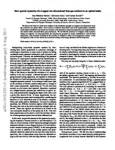
with distance as G(ξ) = A20 (1 + (ξ/α ˜ )2 )−1/(4K0 ) . This behavior is typical of a Luttinger liquid. Then, as the interaction strength is slowly ramped up, the form of the correlation function evolves. For small ξ and sufficiently short τ , changes are minimal as the correlation function still decays algebraically, but the exponent is now determined √ by the timedependent Luttinger parameter K(t) = K0 / τ showing up in the exponent [36]. This result implies that for short dimensionless distances, ξa := τ −1/4 ≫ ξ, the correlations react instantaneously to the slow interaction change and adjust to the ground state decay corresponding to the current interaction value (see panel (a) of Fig. 1). The main contribution to this mechanism comes from quasiparticles with large momenta q ≫ l10 . This adiabatic regime spatially decreases with time and disappears completely when ξa (t) ≈ α ˜ , where α ˜ is the dimensionless short distance cut-off.

1 0 −. 3

∝ (1 + ( αξ˜ ) 2 )

−

√ τ 4K 0

ξB J t ¯h f

τ =3

= 60

1 0 −. 4

1 0 −. 4 1

ξ

10

1

ξ

10

FIG. 1: Decay of single-particle correlations with increasing distance for different τ and tf . Comparison between results obtained using bosonization Eq. (7) with Luttinger liquid parameters K0 = 4.1561 and u0 = 1.3323 (solid lines) and using timedependent density-matrix renormalization group (t-DMRG) for the Bose-Hubbard model (circles) for a quench from U0 = J (lattice length: L = 100, filling: n = 1, maximum number of bosons per site: 6). (a) Time evolution for different values of τ and for a fixed value of tf = 40 J~ . The two dashed lines intersecting all τ data sets are the bounds: (left) ξa = τ −1/4 and (right) ξB = 2(τ 3/2 − 1). The colored dashed lines on the left of ξB are proportional to the function (1 + ( αξ˜ )2 )−1/(4K(τ )) ; while the dashed lines on the right of ξB are proportional to the function ξ −1/(2K0 ) . (b) Comparison between different ramp times tf for a fixed value of τ = 3. The vertical dashed line is the bound ξB = 2(τ 3/2 − 1).

Asymptotic expansion of the single-particle correlation function: The time evolution of single-particle correlations described by Eqs. (7) and (8) is extremely rich. Typical time evolutions of these correlations with distance are shown in panel (a) of Fig. 1 for both the Bose-Hubbard model and the bosonization approach. For the chosen parameters, we found very good agreement between the two evolutions at longer distances, as long as an additional time-dependent prefactor is multiplied to the expression obtained using bosonization. This prefactor corrects for the short distance behavior which is not properly taken into account by the low energy theory. As expected, the bosonization description works best for slow and small parameter changes. In particular, deviations are observed when the Mott-insulating phase of the Bose-Hubbard model is approached or when too many excitations are created. Initially, before the slow quench begins (at τ = 1 within our formalism), the correlation function decays algebraically

For larger distances, the correlations deviate much more from their standard initial form and a dip appears. The formation of this dip is a clear signal of the non-equilibrium nature of the physics at play. For distances beyond this dip, the initial algebraic decay, ξ −1/(2K0 ) , reappears as one can see in panel (a) of Fig. 1. The position of the dip coincides approximately with the correlation evolution front. The time-dependent position of this front can be understood by considering the propagation of quasiparticles. At any given time t, the system Hamiltonian P is diagonal in its instantaneous quasiparticles as H(t′ ) = q u(t′ )|q|a†q (t′ )aq (t′ ) + 21 . Assuming discrete time steps, this means that the action of the Hamiltonian at time t − δt, diagonal in its own quasiparticles, has created (and annihilated) entangled quasiparticle pairs a†q (t)a†−q (t). These entangled quasiparticles, forming a pair, propagate with velocity u(t) in opposite direction and thereby carry correlations over a distance 2 u(t) dt within a time interval dt. Hence, for points separated by a distance Rt ξ larger than ξB = l30 0 dt′ u(t′ ), the single-particle correlation decay is unaffected by the change in the interaction aside fromqan overall prefactor. For the system under study, u(t) = u0 1 + tt0 and we find that ξB = 2 (τ 3/2 − 1). Thus, the evolution front beyond which correlations still follow the initial algebraic decay is given by ξB as evidenced in Fig. 1. In particular, the position of the bound does not depend on the ramp velocity and time separately as can be seen in panel (b) of Fig 1. One clearly sees from there that, for a given τ , the position ξ of the dip (measured in units of l0 ) is the same for different ramp times. The existence of such a propagation front is reminiscent of the light-cone-like evolution of correlations recently investigated in the context of instantaneous quenches [24, 25, 37–40].

For larger dimensionless times, as illustrated in Fig. 2, an additional decay regime takes place at intermediate distances before the bound ξB . This interesting behavior shows up in

4 1 3

ξ B = 2(τ 2 − 1)

10 − 5

τ K 02

G(ξ , τ )

10

= 20

−10

10 − 1 5

τ K 02

= 40

10 − 2 0

10

τ K 02

= 60

τ K 02

= 100

fi rst term on l y

−25

10 − 3 0 0

100

200

ξ

300

400

500

FIG. 2: Behavior of single-particle correlations with increasing distance for large values of τ /K02 . Exact evaluation of the bosonization expression, Eq. (8) – solid lines, is compared to the full approximate expression, Eq. (9) – dashed lines. For τ /K02 = 100, we also compare the exact expression to the first exponential term of Eq. (9). In the large τ limit, if one adjusts the prefactor correctly, the stretched exponential provides a good description of the correlation decay before ξB . The black dashed line indicates the position of the evolution front ξB = 2 (τ 3/2 − 1). Used parameters: smin = 10−5 , smax = 60 (the lower and upper cut-offs in Eq. (8)) and α ˜ = 0.1.

the bosonization approach and takes the form ˜ )× G(ξ, τ )q≃0 ≃ C(τ 1 3

exp −

1 2

1 2 π2 τ ξ3 K0 Γ( 31 )3

!

3 2

exp

1 2

π τ Γ( 61 ) 1 1 6K0 Γ( 31 )Γ( 23 )2 ξ 3

(9) !

˜ ) a prefactor independent of ξ. For intermediate τ , with C(τ both exponential terms are required to adequately reproduce the behavior of Eq. (8) as shown in Fig. 2. However, for values of τ whose corresponding bound ξB is located at sufficient large ξ, only the first exponential term is important. In this case single-particle correlations decay with distance as a stretched exponential, a similar decay was found in Ref. 16. Such a functional form is unconventional for Luttinger liquids as, typically, correlations decay algebraically in these systems. Even for sudden interaction quenches in both bosonic and fermionic systems [26, 41] and for slow quenches in fermionic systems [19], only algebraic decay of correlations have been uncovered. The presence of such an unusual functional form is mainly due to the contribution of quasiparticles with momenta around 1 3 2ξB l0 < q ≤ l0 [36]. Moreover, as the appearance of the stretched exponential decay is limited to large values of τ , this regime only occurs for relatively large parameter changes t ≫ t0 . It is still an open question, whether this stretched exponential decay regime arises within the Bose-Hubbard model. As this regime only occurs for large parameter changes, the TLL model might not describe properly the dynamics of the BoseHubbard model and relaxation mechanisms not present in the

TLL model might dominate the evolution. A careful analysis of this last point would be extremely valuable but is left to further studies. Experimental implementation and detection: Onedimensional interacting bosonic gases have been realized experimentally using a few different setups [42–44]. The best scheme to implement time variations of the interaction strength depends on the actual experiment setup. One method relies on the use of a Feshbach resonance by which the scattering length, and thereby the interaction strength, is directly varied. A second technique is based on the application of a weak optical lattice suppressing the tunneling amplitude in order to change the ratio of the interaction strength to the kinetic energy. Finally, in one-dimensional wave guides, geometric confinement can be employed to tailor the interaction strength. The detection of the single-particle correlation function can also be carried out experimentally. Using radio-frequency pulses, atoms can be outcoupled from the one-dimensional Bose gas at two spatially separated positions and their interference is then observed after a free fall. This technique was successfully employed to measure the build-up of equaltime single-particle correlations in a Bose-Einstein condensate after a sudden decrease of its temperature and the critical correlations at the phase transition [45, 46]. Another possible detection scheme relies on time-of-flight (TOF) measurements which provide, in the far-field limit, access to the moR mentum distribution n(q) = dx eiqx G(x). The very long distance behavior of the single-particle correlation is dominated by the Luttinger liquid power-law; however, at a critical wavevector, qc , determined by the ballistic expansion condition, a crossover occurs and n(q) is dominated by the Fourier transform of the stretched exponential. Therefore, at qc ∼ mB ξB l0 /t (with mB the atom mass) a crossover should be visible in the TOF measurements. We foresee that one of the main challenges towards the observation of the evolution of correlations will be the realization of a relatively homogeneous gas as inhomogeneities can cause mass transport and mask the internal evolution [22, 47]. Conclusion: We carefully studied the dynamics of singleparticle correlations arising during the slow interaction quench of a one-dimensional Bose gas using both a bosonization approach and numerical simulations for the BoseHubbard model. We uncovered various regimes: for short distances, we found single-particle correlations to decay algebraically with an exponent which depends on the ramp time; while for intermediate distances but at long times, the decay of correlations follows a stretched exponential. This unconventional regime is bounded by an evolution front, reminiscent of a Lieb-Robinson bound, whose dynamics is dictated by the counter-propagation of entangled quasiparticle pairs. The existence of this regime within the Bose-Hubbard model remains an open question. Deviations between the BoseHubbard and Luttinger models were in fact found for fast as well as for very long ramps. Finally, beyond this evolution front, correlations decay algebraically with an exponent given

5 by the sudden approximation. These results may serve as a basis for comparison with future experimental studies of unconventional time evolutions in many-body one-dimensional systems. We are grateful to T. Giamarchi for helpful discussions and to G. Roux for his insights on related works. We acknowledge support from ANR (FAMOUS), SNFS under MaNEP and Divison II, NSERC of Canada and CIFAR.

[1] H. Lignier, C. Sias, D. Ciampini, Y. Singh, A. Zenesini, O. Morsch, and E. Arimondo, Phys. Rev. Lett. 99, 220403 (2007). [2] D. N. Basov, R. D. Averitt, D. van der Marel, M. Dressel, and K. Haule, Rev. Mod. Phys. 83, 471 (2011). [3] J. Struck, C. lschlger, R. Le Targat, P. Soltan-Panahi, A. Eckardt, M. Lewenstein, P. Windpassinger, and K. Sengstock, Science 333, 996 (2011). [4] J. T. Barreiro, M. Mller, P. Schindler, D. Nigg, T. Monz, M. Chwalla, M. Hennrich, C. F. Roos, P. Zoller, and R. Blatt, Nature 470, 486 (2010). [5] N. Syassen, D. M. Bauer, M. Lettner, T. Volz, D. Dietze, J. J. Garcia-Ripoll, J. I. Cirac, G. Rempe, and S. D¨urr, Science 320, 1329 (2008). [6] M. Greiner, O. Mandel, T. W. H¨ansch, and I. Bloch, Nature (London) 419, 51 (2002). [7] C.-L. Hung, X. Zhang, N. Gemelke, and C. Chin, Phys. Rev. Lett. 104, 160403 (2010). [8] J. F. Sherson, C. Weitenberg, M. Endres, M. Cheneau, I. Bloch, and S. Kuhr, Nature (London) 467, 68 (2010). [9] W. S. Bakr, A. Peng, M. E. Tai, R. Ma, J. Simon, J. I. Gillen, S. F¨olling, L. Pollet, and M. Greiner, Science 329, 547 (2010). [10] D. Chen, M. White, C. Borries, and B. DeMarco, Phys. Rev. Lett. 106, 235304 (2011). [11] A. Polkovnikov, K. Sengupta, A. Silva, and M. Vengalattore, Rev. Mod. Phys. 83, 863 (2011). [12] R. Sch¨utzhold, M. Uhlmann, Y. Xu, and U. R. Fischer, Phys. Rev. Lett. 97, 200601 (2006). [13] F. M. Cucchietti, B. Damski, J. Dziarmaga, and W. H. Zurek, Phys. Rev. A 75, 023603 (2007). [14] L. Cincio, J. Dziarmaga, M. M. Rams, and W. H. Zurek, Phys. Rev. A 75, 052321 (2007). [15] R. W. Cherng and L. S. Levitov, Phys. Rev. A 73, 043614 (2006). [16] A. Polkovnikov and V. Gritsev, Nature Physics 4, 477 (2008). [17] M. Eckstein and M. Kollar, New Journal of Physics 12, 055012 (2010). [18] M. Moeckel and S. Kehrein, New Journal of Physics 12, 055016 (2010). [19] B. D´ora, M. Haque, and G. Zar´and, Phys. Rev. Lett. 106, 156406 (2011). [20] J. Dziarmaga and M. Tylutki, Phys. Rev. B 84, 214522 (2011). [21] D. Poletti and C. Kollath, Phys. Rev. A 84, 013615 (2011). [22] J.-S. Bernier, D. Poletti, P. Barmettler, G. Roux, and C. Kollath, Phys. Rev. A 85, 033641 (2012). [23] E. H. Lieb and D. W. Robinson, Communications in Mathematical Physics 28, 251 (1972). [24] P. Calabrese and J. Cardy, Phys. Rev. Lett. 96, 136801 (2006). [25] M. Cheneau, P. Barmettler, D. Poletti, M. Endres, P. Schauß, T. Fukuhara, C. Gross, I. Bloch, C. Kollath, and S. Kuhr, Nature

481, 484 (2012). [26] M. A. Cazalilla, Phys. Rev. Lett. 97, 156403 (2006). [27] I. Bloch, J. Dalibard, and W. Zwerger, Rev. Mod. Phys. 80, 885 (2008). [28] C. Kollath, U. Schollw¨ock, J. von Delft, and W. Zwerger, Phys. Rev. A 69, 031601 (2004). [29] T. Giamarchi, Quantum Physics in One Dimension (Oxford University Press, Oxford, 2004). [30] M. A. Cazalilla, R. Citro, T. Giamarchi, E. Orignac, and M. Rigol, Rev. Mod. Phys. 83, 1405 (2011). [31] E. H. Lieb and W. Liniger, Phys. Rev. 130, 1605 (1963). [32] T. D. K¨uhner and H. Monien, Phys. Rev. B 58, R14741 (1998). [33] F. D. M. Haldane, Phys. Rev. Lett. 47, 1840 (1981). [34] M. Abramowitz and I. Stegun, eds., Handbook of mathematical functions (Dover, New York, 1972). [35] Equivalently, the solution can be expressed using Airy functions, but the Bessel function representation leads to a more straightforward derivation of asymptotics. [36] J.-S. Bernier, R. Citro, C. Kollath, and E. Orignac, Supplementary material for Correlation dynamics during a slow interaction quench in a one-dimensional Bose gas, attached to this manuscript (2013). [37] E. H. Lieb and D. W. Robinson, Commun . Math. Phys. 28, 251 (1972). [38] S. Bravyi, M. B. Hastings, and F. Verstraete, Phys. Rev. Lett. 97, 050401 (2006). [39] A. M. L¨auchli and C. Kollath, J. Stat. Mech.: Theor. Exp. 5, 18 (2008). [40] E. H. Lieb and A. Vershynina, arXiv:1306.0546 (2013). [41] C. Karrasch, J. Rentrop, D. Schuricht, and V. Meden, Phys. Rev. Lett. 109, 126406 (2012). [42] T. St¨oferle, H. Moritz, C. Schori, M. K¨ohl, and T. Esslinger, Phys. Rev. Lett. 92, 130403 (2004). [43] B. Paredes, A. Widera, V. Murg, O. Mandel, S. F¨olling, I. Cirac, G. V. Shlyapnikov, T. W. H¨ansch, and I. Bloch, Nature 429, 277 (2004). [44] T. Kinoshita, T. Wenger, and D. S. Weiss, Science 305, 1125 (2004). ¨ [45] S. Ritter, A. Ottl, T. Donner, T. Bourdel, M. K¨ohl, and T. Esslinger, Phys. Rev. Lett. 98, 090402 (2007). ¨ [46] T. Donner, S. Ritter, T. Bourdel, A. Ottl, M. K¨ohl, and T. Esslinger, Science 315, 1556 (2007). [47] S. S. Natu, K. R. A. Hazzard, and E. J. Mueller, Phys. Rev. Lett. 106, 125301 (2011).

1

Supplementary material DERIVATION OF EQ. (8) OF THE MAIN TEXT

Within the bosonization formalism the equal-time single-particle correlation function is G(x, t)q≃0 = A20 heiθ(x,t) e−iθ(0,t) i 1

2

= A20 e− 2 h(θ(x,t)−θ(0,t)) i .

(S1)

The correlator appearing above is obtained from Eqs. (4) and (5) of the main text and is given by 2 Z +∞ 1 dq −α|q| d 2 e F (q, t) [1 − cos(qx)] h(θ(x, t) − θ(0, t) i = 2 3 2K0 u0 −∞ |q| dt

(S2)

where the derivative of Eq. (6) of the main text is √ h  i d 3 u0 3 3 3 3 πτ s2 J 32 (s) J− 23 (sτ 2 ) − J− 32 (s) J 32 (sτ 2 ) + i J− 31 (s)J− 23 (sτ 2 ) + J 31 (s) J 23 (sτ 2 ) F (q, t) = dt 2 l0

with Jn (y) the Bessel function of the first kind. Recall that l0 = u0 t0 is the typical lengthscale, s(q, t0 ) = 23 l0 |q| the dimensionless momentum, and τ (t, t0 ) = 1 + tt0 the dimensionless time. ASYMPTOTIC EXPANSIONS 1

˜ In order to obtain analytical approximations for the single-particle function G(x, t)q≃0 = A20 e− 2 I(ξ,τ,α) , we need to approx2 2 − 32 2 − 32 ≪ s ≪ 3 and s ≫ 23 (note that τ ≥ 1 imate the integral I(ξ, τ, α). ˜ We identify three important regimes: s ≪ 3 τ , 3 τ and that we separate the regimes in s at 23 instead of 1 as this corresponds to a splitting at 1l 0 in momentum space). These three regimes determine the size of the arguments of the Bessel functions entering the integral I(ξ, τ, α ˜ ). Therefore, we split this inte3 3 gral into three parts I(ξ, τ, α) ˜ = G (ξ, τ )+H (ξ, τ )+Q(ξ, τ ) with G(ξ, τ ) = I(ξ, τ, α ˜ , 0, 23 τ − 2 ), H(ξ, τ ) = I(ξ, τ, α ˜ , 32 τ − 2 , 32 ), 2 and Q(ξ, τ ) = I(ξ, τ, α, ˜ 3 , ∞) using Z π 2 τ 2 c2 ˜ I(ξ, τ, α, ˜ c1 , c2 ) = ds s e−αs [1 − cos(sξ)] × (S3) 3K0 c1  2  2  3 3 3 3 . J 32 (s)J− 32 (sτ 2 ) − J− 23 (s)J 23 (sτ 2 ) + J− 13 (s)J− 23 (sτ 2 ) + J 31 (s)J 23 (sτ 2 )

The Bessel functions of the first kind can take simpler approximated forms (using expressions taken from Ref. 1) in the two following regimes:  s ν 2 1 for s ≪ , Jν (s) ∼ , (S4) 3 2 Γ(ν + 1) r h i 2 2 π for s ≫ , Jν (s) ∼ cos s − (2ν + 1) . (S5) 3 πs 4 Large momentum contribution

For the function Q(ξ, τ ) which covers the regime s ≫ 23 , we get         Z +∞ 2 2 2 1 1 ds 1 −sα ˜ E1 E1 [1 − cos(sξ)]e = α ˜ − (˜ α + iξ) + E1 (˜ α − iξ) , (S6) Q(ξ, τ ) ≃ K(τ ) 2/3 s K(τ ) 3 2 3 3 where K(τ ) =

K0 √ τ

and E1 is the exponential integral function [1]. For ξ ≪ 1, we find   1 ξ2 Q(ξ, τ ) ≃ ln 1 + 2 , 2K(τ ) α ˜

(S7)

2 while for ξ ≫ 1, Q(ξ, τ ) ≃

  −γE   e 1 1 −2 ln sin (ξ) + O(ξ ) + 2 K(τ ) ξ ˜ 3α

(S8)

where γE is Euler’s constant. Small momentum contribution

For the small momentum contribution, given by G(ξ, τ ), we obtain the following expression −3 Z 2ξ 2 3 τ 1 du G (ξ, τ ) ≃ [1 − cos u] K0 0 u   2ξ 1 1 Cin ≃ . K0 3 τ 32

(S9)

Intermediate momentum contribution

The most interesting contribution is the intermediate momentum one which is due to H(ξ, τ ). This expression simplifies to √ √ 5 7 3 3 23 π τ 23 π τ 2 2 (S10) H (ξ, τ ) ≃ 1 2 Φ1 (ξ, τ ) + 2 2 Φ2 (ξ, τ ) 3K0 (Γ( 3 )) 3K0 (Γ( 3 )) where 3 2

Φ1 (ξ, τ ) = 3

Φ2 (ξ, τ 2 ) =

Z Z

2 3 3 2 −2 3τ 2 3 3 2 −2 3τ

ds s

4 3

ds s

2 3

3

[1 − cos(sξ)] sin2 (sτ 2 − 3

[1 − cos(sξ)] cos2 (sτ 2 +

π ), 12

(S11)

π ). 12

(S12)

In the limit where τ ≫ 1 and ξ ≫ 1, this expression can be further simplified and we find !  1 ! 1 1 1 2 4 Γ( 13 ) 3 3 π 2 Γ( 61 ) 1 1 1 2 2 3 πτ 2 2 3 π2 τ 2 ξ3 − 23 33 − 2 1 1 , + H (ξ, τ ) ≃ π 2 K0 Γ( 31 )3 3 K0 Γ( 32 )2 2 3 Γ( 3 ) ξ 3 whereas in the limit where τ ≫ 1 and ξ ≪ 1, we find √ τ H (ξ, τ ) ≃ 4π K0

1 5

5 3 3 Γ( 13 )2

+

1 7

7 3 3 Γ( 32 )2

!

ξ2.

(S13)

(S14)

Approximation for the full single-particle correlation function 1

The full single-particle correlation function is given by G(x, t)q≃0 = A20 e− 2 (G(ξ,τ )+H(ξ,τ )+Q(ξ,τ )) . We now use the expressions derived above to find approximations for the entire function. 3

(i) Let us first discuss the limit of large distances such that ξ ≫ τ 2 (which necessarily implies that ξ ≫ 1). In this limit, the large and intermediate momentum contributions become, to first order, independent of ξ while the low momentum   2ξ − 23 1 1 contribution G(ξ, τ ) ≃ K0 Cin 3 τ ≃ K0 (γE + ln(ξ)) dominates. Thus the single-particle correlation behaves as G(ξ, τ )q≃0 ≃ A(τ )

  2K1 0 1 ξ

(S15)

where A(τ ) is a function which depends on τ . We see that the Luttinger liquid behavior is recovered for long distances and that the exponent is the one expected in equilibrium before the ramp.

3 1

(ii) Let us now discuss the case of small distances ξ ≪ τ − 4 . In this limit, one obtains that the large momentum contribution, Q(ξ, τ ), dominates since the intermediate and small momentum contribution vanish algebraically. Thus the correlation is well described by the expression 

2

G(ξ, τ )q≃0 ≃ B(τ ) 1 +

ξ α ˜2

√

− 4Kτ

0

(S16)

with B(τ ) a function depending on τ . (iii) For intermediate distances, finding an asymptotic expression for the single-particle correlation is a more subtle task. 3 However, for 1 ≪ ξ ≪ τ 2 , one obtains "   1 !# 1 1 Γ( 31 ) 3 3 1 2 3 π2 τ 2 3 G(ξ, τ )q≃0 ≃ C(τ ) exp − ξ − (S17) π 2 K0 Γ( 13 )3 " !# 1 1 π 2 Γ( 16 ) 1 2 πτ 2 1 × exp − 1 23 33 − 2 1 1 . 3 2 3 K0 Γ( 32 )2 2 3 Γ( 3 ) ξ 3 where C(τ ) a function that depends on τ . This expression is due to the contribution H(ξ, τ ) at intermediate momentum, and for sufficiently large ξ the first exponential is dominant. FOURIER TRANSFORM OF A STRETCHED EXPONENTIAL β

The Fourier transform of a stretched exponential function of the form f (x) = e−x with β < 1 is given by the expression ∞

∞ Z X

∞

∞

∞

∞

X (−1)n Γ(βn + 1) π uβn eiu = ei 2 (βn+1) βn+1 βn+1 q Γ(n + 1) q 0 0 0 0 0 (S18) Γ( n 1 3 +1) which is a convergent sum. When β = 3 , the sum can be further evaluated by using properties of the Γ functions, Γ(n+1) = Q(q) =

n 1 Γ( 3 ) 3 Γ(n) ,

Z

β

dxe−x eiqx =

(−xβ )n iqx X (−1)n e = n! n! 0

Z

du

and definitions of the Hypergeometric functions [1], this exercise yields the result   −i π sign(q)  π π πe−i 6 sign(q) e−i 2 sign(q) −e 6 1− Q(q) = Hi 1 1 |q| (3|q|) 3 (3|q|) 3

where Hi is the Scorer function [1–3].

[1] M. Abramowitz and I. Stegun, eds., Handbook of mathematical functions (Dover, New York, 1972). [2] A. Gil, J. Segura, and N. M. Temme, Math. Comp. 70, 1183 (2001). [3] A. I. Nikishov and V. I. Ritus, math-ph/0501062 (2005).

(S19)