Correlation Exploitation in Error Ranking - Stanford University

Correlation Exploitation in Error Ranking Ted Kremenek, Ken Ashcraft, Junfeng Yang and Dawson Engler Computer Systems Laboratory Stanford University Stanford, CA 94305, U.S.A.

ABSTRACT

1. INTRODUCTION

Static program checking tools can find many serious bugs in software, but due to analysis limitations they also frequently emit false error reports. Such false positives can easily render the error checker useless by hiding real errors amidst the false. Effective error report ranking schemes mitigate the problem of false positives by suppressing them during the report inspection process [17, 19, 20]. In this way, ranking techniques provide a complementary method to increasing the precision of the analysis results of a checking tool. A weakness of previous ranking schemes, however, is that they produce static rankings that do not adapt as reports are inspected, ignoring useful correlations amongst reports. This paper addresses this weakness with two main contributions. First, we observe that both bugs and false positives frequently cluster by code locality. We analyze clustering behavior in historical bug data from two large systems and show how clustering can be exploited to greatly improve error report ranking. Second, we present a general probabilistic technique for error ranking that (1) exploits correlation behavior amongst reports and (2) incorporates user feedback into the ranking process. In our results we observe a factor of 2-8 improvement over randomized ranking for error reports emitted by both intra-procedural and inter-procedural analysis tools.

Recently there has been a surge of interest in using static checking to find program errors [1, 3, 5, 9, 11–15, 23, 24]. A practical problem with these tools is that in flagging true errors they also flag false ones. These false reports (“false positives”) can quickly render tools useless by hiding real errors amidst the false, potentially causing the tool to be discarded as irrelevant. Empirically, tools that effectively find errors have false positive rates that can exceed 30% [10, 13, 15, 24]. Typically, such tools are used as follows: (1) the tool is run and emits error reports, (2) these reports are ordered using some sort of ranking scheme [17, 19, 20] and (3) the programmer inspects the error reports, eliminating false ones. Ideally, all the reports the user inspects are true errors. In practice, industrial-strength tools aim to minimize the impact of false positives by sorting reports so that the end-user inspects as many bugs (and as few false positives) as possible. In this way the initial inspections have a high number of bugs; users can inspect errors until the false positive rate becomes “too high” and then stop. A major weakness of all current ranking schemes is that they are “static” in that they do a one-time sorting of error reports that are then presented for user consumption. Unfortunately, they squander the useful feedback given by the user during inspection when they manually classify reports as false or valid. By exploiting strong correlations among reports, feedback allows reports to be dynamically reordered after each inspection, potentially dramatically improving ranking quality. Moreover, as a codebase evolves and a checking tool is continually applied, the tool will emit new reports, many of which will correlate with reports inspected during a previous application of the tool. If previously inspected reports correlate strongly with newly emitted ones, the feedback from prior inspections can also improve the initial sorting of the newly emitted reports. Our main source of leverage is that error reports are highly correlated by code locality, and they can be logically grouped into sets of (possibly overlapping) highly correlated populations. Populations are groups of related reports, and together they serve to partition the set of all reports emitted by a tool. An example of a population is the set of error reports that indicate the occurrence of bugs in a specific function, while another population may be all of the error reports for code that had a high degree of recent developer activity. Because reports are correlated within a population, inspecting one message from a given population yields

Categories and Subject Descriptors D.2.4 [Software/Program Verification]: Statistical methods—error ranking; G.3 [Probability and Statistics]: Correlation and regression analysis

General Terms Verification, Measurement

Keywords program checking, static analysis, error ranking

Permission to make digital or hard copies of all or part of this work for personal or classroom use is granted without fee provided that copies are not made or distributed for profit or commercial advantage and that copies bear this notice and the full citation on the first page. To copy otherwise, to republish, to post on servers or to redistribute to lists, requires prior specific permission and/or a fee. SIGSOFT’04/FSE-12, Oct. 31–Nov. 6, 2004, Newport Beach, CA, USA. Copyright 2004 ACM 1-58113-855-5/04/0010 ...$5.00.

information about the others. For example, if the messages in a population are perfectly correlated, then classifying one effectively classifies them all. If the message was a false positive, so are the others and they should be skipped. If it it was a true error, so are the others and the user should fix them. Properly exploited, even less perfect correlations can dramatically amplify the information gained from a single inspection. In practice, messages cluster at a variety of levels. For example, we expect both messages within the same file and within the same function to be correlated. Programmers that make a mistake once may well do so repeatedly either because they are poor programmers or simply unaware of a checked rule. Similarly, a static analysis mistake may repeat because surrounding code will contain the same construct that caused the problem. This paper makes two contributions. First, it experimentally demonstrates that true and false error reports are highly correlated by code locality. We gather correlation data using a variety of program checkers on two large systems: Linux, an open-source operating system, and “System X,” a commercial, closed-source system. The checkers differ both in the class of properties they check and in the degree of analysis sophistication they use, ranging from intraprocedural flow-sensitive checkers to inter-procedural path sensitive ones. The high correlation of messages holds across all these views. Its second contribution is that we present a probabilistic ranking technique called Feedback-Rank that effectively exploits the correlation among reports and reduces the number of false positives a user encounters during inspection (on average by a factor of 2-8 over randomized ranking, with close to optimal ranking in some cases). The technique is probabilistic because correlations are frequently noisy; reports are often highly—but not perfectly—correlated, and we require a technique that allows us to soundly reason about multiple sources of uncertainty. It employs a flexible probabilistic model called a Bayesian Network [8]. We use it to model correlation among reports based on population groupings, but it can easily be expanded to model other sources of correlation as well. As presented in this paper, ranking expands to three stages: (1) grouping error reports into sets of correlated populations, (2) choosing an initial order for reports (similar to current ranking schemes), and (3) selecting which report to inspect next given the information gained from the previous inspections. This inspection strategy has several nice features. First, it does not depend on the internals of the checking system but can simply work with the tool’s output. Thus, it is immediately portable to other program checkers where the same correlation assumptions hold (as we expect them to from ample anecdotal evidence). Second, it makes even tools that generate an exceptional number of false reports usable as long as these reports are correlated in some way. For example, an infinite population of perfectly correlated false reports is inconsequential since you can suppress all of them after the first inspection. Currently, tools must generate a low number of false positives to be useful, which is a much stronger requirement. Thus, the strategy makes it so that the number of false error reports does not necessarily matter, the important features are (1) the number of different populations (since each must be observed at least once) and (2) the strength of the correlation between messages in these populations. In practice,

the correlation tends to be high enough that the main thing that matters is the number of populations rather than the number of false positives. Third, the strategy works well initially, yet improves with use. As users spend more time inspecting more errors, it is able to customize itself post facto to the observed data, thereby improving its ability to classify future data from the same system. This paper is organized as follows. In Section 2 we present a statistical analysis of correlations among error reports based on code locality. In Section 3 we discuss our ranking strategy Feedback-Rank and in Section 4 we describe the probabilistic model in detail that is used for the ranking process. Section 5 provides our experimental results. We discuss related work in Section 6 and conclude in Section 7.

2. DATA ANALYSIS This section analyzes two large databases of error reports to demonstrate that true errors and false positives frequently cluster by code locality. Along with an intuition as to why clustering would happen, we provide a graphical representation and a statistical analysis of the clustering in these error reports.

2.1 Correlation Intuition Intuitively, we expect bugs to cluster because programmers that make one mistake are relatively likely to make more. In addition, if programmers do not know a rule, they will repeatedly violate it given the chance. The most egregious example we have encountered is in the Linux kernel, which has the rule “do not call a blocking function with interrupts disabled.” Programmers unaware of the rule, or that a given function blocks, violate it enthusiastically — we have observed routines that have 17, 23, and 28 errors of this type. These types of clustering are also common with security rules, of which programmers are often unaware. Like bugs, false positives also cluster, though here the culprit is the analysis rather than the programmer. False positive correlation comes from three sources. First, analysis mistakes often generate a cascade of false reports rather than just one. In an extreme case in Linux 2.4.1, our lock checker analysis that checks if a lock can be double acquired could not handle a recursive lock in drivers/usb/uhci.c, resulting in 14 false positives in that file. In related work, z-ranking, a static error report ranking scheme, uses statistical heuristics to identify such “explosions” of false positives [20]. More commonly, however, analysis mistakes lead to two or three false positives. Thus, knowing that one error report is false allows the user to ignore the others. The second source is that analysis mistakes often happen because of unanticipated or “rare” coding idioms (anticipated, common ones can be tuned for) — in this case, if a programmer uses a problematic idiom once, it is likely that they will do so again, causing more problems. The third source is that checked rules may not always be 100% correct; certain special contexts may violate them safely, but will be flagged repeatedly by the checker. For example, memory allocators may not need to be checked for failure in boot-up initialization code. More generally, the false positives stem from either an incomplete specification (where the rule is only approximate) or the tool is not precise enough to capture all the reasoning to correctly verify the specification. The former often occurs in practice as the many “edge-cases” and

Class

Check

Function Pairs

Lock Alock A-B

System

Bugs

FPs

L X L X

16 3 11 2

50 34 37 11

Rule Checked Release acquired locks; do not double-acquire locks.

14 17 14

6 27 3

Do not use freed memory.

161

20

To avoid deadlock, do not call blocking functions with interrupts disabled or a spinlock held. Restore disabled interrupts.

Same as Lock, but checks an analytically inferred set of locking functions. Pair function A with a call to B.

Memory

Free Inverse

L X X

Interrupts

Block

L

Intr

L

27

49

Null

122 210 31 25

48 15 25 23

Check potentially NULL pointers returned from routines.

Internal-null Rev-inull

L X X X

User Values

Param Range

L L

7 54

14 4

Do not dereference user pointers. Always check bounds of array indices and loop bounds derived from user data.

System Specific

Exc-none Format

X X

2 28

72 98

Proprietary Use constant format strings.

Null Pointers

Roll back changes on error paths.

Do not dereference null pointers. Do not dereference a pointer and then check it for NULL.

Table 1: Checkers used in our analysis organized by class of errors and system (“L” for Linux 2.4.1, “X” for System X). The number of true bugs and false positives (FPs) are listed for each checker. exceptions to a rule in a system are often not fully documented or understood by the writer of the checking tool.

2.2 The Data We use the error reports from two systems, Linux 2.4.1 and a large anonymous commercial system, System X. System X is a large (≈ 800K lines of code), complex system that contains elaborate locking patterns, strict memory management, and validation of all input from untrusted sources. The data is the manually classified error reports from the checkers in Table 1. The data comes from previous work on the xgcc compiler [10]. We gathered the reports over many months of continuous checking of these systems. Each report includes the file, function name and line number. We use this information to measure clustering and to group reports.

2.3 The Checkers This section characterizes some of the checkers from Table 1 to show how their bugs and false positives cluster. The “Function Pairs” class of checkers enforced rules like “calls to locking functions must be followed by calls to unlocking functions.” While these checkers were able to find over 30 bugs total, they were often confused by false paths in the code. For example, the following data-dependency idiom is common and causes the immature versions of these checkers used for this study to believe that there are actually four paths through the function instead of just two: if (do lock) lock(); // Do some work if (do lock) unlock(); Mature, more path-sensitive versions of these checkers can now handle this case. Because this troublesome idiom was so common, these analysis mistakes were highly correlated. The checkers in the Memory class, on the other hand, were much more likely to find clusters of bugs than false positives. For example, the Inverse checker looks for places where the developer makes one or more resource allocations and then forgets to free those resources along an error path. If the developer forgets to free along one error path, he commonly will forget it along the other error paths in the function. The types of rules checked in this study are very similar

to those checked by related work [1, 3, 5, 11–13, 15, 23, 24]. We expect that those analyses will find clusters of bugs because we have found clusters of the same types of bugs that they find. We expect that those analyses will find clusters of false positives because those analyses do make mistakes, and some of them [11,12,15,23, 24] went so far as to classify the false positives into several groups. Therefore, those analyses could leverage clustering in the error report inspection process.

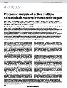
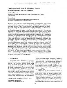
2.4 Observed Clustering With an intuition as to why clustering would occur, we can now examine how to actually cluster reports. There are many ways we can cluster reports together. This includes version control data, code churn, and other sources. In this paper, we have chosen to focus on clustering by code locality. We felt the data we possessed was accurate enough to study such clustering, and such clustering is easily exploitable for ranking on any codebase. This subsection graphically represents the clustering by code locality present in the two datasets. We split the data into populations based on code locality using three (arguably coarse) partitions: (1) function, (2) file, and (3) leaf-directory. The “function” partition groups all reports together that indicate there is an error in a specific function. The definition is analogous for the other two groupings, where a “leaf-directory” is the directory that contains a file and function where a flagged error occurred. Each report is therefore part of three populations, one of each type. Figures 1 and 2 show the number of populations across all checkers with a given number of bugs and false positives for Linux and System X respectively. Each subgraph represents the different types of populations (function, file, leaf directory), while each circle represents the number of populations that contained a given number of bugs and false positives. For example, Figure 1(a) shows that there were 42 functions in Linux that contained 2 bugs and 0 false positives. It is important to note the “L” shape formed by the data in Figures 1(a) and 2(a). The “L” means that there are very few populations that contain a mix of bugs and false posi-





























































(a) Linux - Grouped by Function

(a) System X - Grouped by Function

(b) Linux - Grouped by File

(b) System X - Grouped by File

(c) Linux - Grouped by Leaf Directory

(c) System X - Grouped by Leaf Directory

Figure 1: Linux 2.4.1 population counts

tives. Most function populations contain few total reports, but usually they are either all bugs or all false positives. We expect that error reports in the same function are likely caused by similar reasons and therefore are either all bugs or all false positives. Note also that the “L” is less visible in the file and directory graphs because our population grouping is more coarse, decreasing the correlations amongst error reports. As our population grouping becomes more coarse, however, we see fewer singleton populations (one error report). Singletons are bad for online ranking because inspecting the lone report tells us nothing about other reports. We now quantify our observations.

2.4.1 Applicability Applicability is defined as the percentage of error reports that are not singletons. To define applicability, there are four key regions we identify in the plots in Figures 1-2: • Region I: Singleton populations (populations consisting of only one error report)

Figure 2: System X population counts • Region II: Non-singleton populations with only false positives • Region III: Non-singleton populations with only bugs • Region IV: Non-singleton populations with both bugs and false positives The set of non-singletons are represented by regions II, III, and IV (keep in mind that the circle size in the plots represent a count of populations and not a count of error reports). Therefore, applicability is Applicability =

II + III + IV I + II + III + IV

(1)

While the plots in Figures 1-2 aggregate the data for the checkers, the corresponding graphs for the individual checkers follow the same trend: moderate applicability at the function level, more applicability at the file level, and even more at the directory level. Table 2(a) gives the exact applicabilities for the two systems and shows this trend. Notice that when grouping error reports in System X by leaf directory, only 2% are singletons whereas 65% of the reports are

Code Locality / Grouping System Linux System X

P r(report = bug)

Function

File

Directory

0.35 0.35

0.70 0.82

0.97 0.98

System

P r(report = FP )

Prior

1 bug

2 bugs

1 FP

2 FPs

0.65 —

0.91 < 10−6

0.99 < 10−6

0.78 < 10−6

0.60 0.0061

0.52 —

0.94 < 10−6

0.97 < 10−6

0.72 < 10−6

0.97 < 10−6

Linux Observed probability: Statistical p-value:

(a) Applicability - The percentage of error reports that are not singletons.

System X Observed probability: Statistical p-value:

Code Locality / Grouping System

Function

File

Directory

0.85 0.41 0.91 0.32

0.62 0.27 0.42 0.13

0.15 0.04 0.11 0.02

Linux (Observed) Linux (Random) System X (Observed) System X (Random)

(b) Skew - The percentage of error reports that appear in homogeneous populations. There is significantly more skew in the real datasets than in their random permutations. Table 2: Applicability and Skew for the different population groupings. Applicability increases as the grouping criteria coarsens, while skew decreases as the grouping criteria coarsens. singletons when grouped by function. Section 2.4.2 shows that there is a tradeoff between applicability and the correlation among the error reports. If we simply group the error reports by directory, it is less likely that they are related.

2.4.2 Skew While applicability is necessary for online ranking, the distinct “L” in Figures 1(a) and 2(a) is also essential. Without the “L”, the populations are heterogeneous, and inspecting one member of a population tells us little about the other members. We define skew as the percentage of reports (in non-singleton populations) that appear in completely homogeneous populations: Skew =

II + III II + III + IV

(2)

Like applicability, the trend found in the aggregated graphs was also present in the graphs for the individual checkers: functions have the most skew and directories have the least. Table 2(b) shows that 85% of Linux error reports, when grouped by function, are in completely homogeneous populations. This means that inspecting one error report will likely tell us the validity of the other error reports in that function. Unfortunately, there is low applicability when grouping by function, meaning that we will be able to take advantage of this skew for only a small subset of the reports. Therefore, our online ranking system must account for this tradeoff between applicability and skew. To show that the skew present in our data is not just a “chance” occurrence, we compared it with a randomized distribution of the reports by taking the set of error reports and shuffling them among the populations. This affected the homo-/heterogeneity of the function, file, and leaf directory populations, but it preserved the populations’ sizes. We performed this experiment 1000 times and calculated the average skew for a randomized distribution of reports. Table 2(b) shows the skew we observe for the real distribution of reports is much higher than the random shuffling, indicating that clustering is present.

Table 3: Prior and conditional probabilities (for function populations) of a given error message being a bug or false positive. The “prior” probability is the (number of bugs) / (number of reports).

2.5 Statistical Quantification To more formally quantify the measurements observed in Section 2.4, we calculated the conditional probabilities of an error report being a bug given that we know at least (1) one other error report in the same function is a bug and (2) at least two are bugs. We also computed the same analogous probabilities for false positives. This represents what would happen in an online ranking scheme; as reports are inspected the probability of a report being a bug changes as new information becomes known. In this case, the user knows that there is already another bug or two in the function and now wants to know how likely it is that a report in that function is valid. Probabilities are shown in Table 3. Listed also is the prior probability for each dataset that a randomly chosen report is a bug (i.e., #bugs/#reports). We also employed a statistical test called a Permutation test to measure the statistical significance of the conditional probabilities compared to the prior probabilities [16]. For the test we fixed the number of reports per function, and randomized the distribution of error reports among the functions. We performed this 10 million times, and computed the number of randomized test cases that had the same or greater conditional probabilities. This proportion is the statistical p-value, and the p-values for each conditional probability are listed in Table 3. The p-values are only estimated to finite accuracy, but our estimates show that most of them have p-values less than 10−6 , very strongly supporting the claim that the distribution of reports is not random and that a high degree of clustering exists for both bugs and false positives.1

3. PROBABILISTIC RANKING In this section we present Feedback-Rank, an adaptive, probabilistic ranking scheme that exploits correlation behavior amongst reports. The algorithm is intended to be complementary to static ranking techniques that can be used to generate an initial good sorting of the reports. We now describe the ranking strategy here, and describe how to model the correlations observed in Section 2 in the next section. For each uninspected report we associate with it a probability that it is a bug. Ranking then reduces to sorting reports by their probabilities. More generally, we are sorting reports by a score value. In static rankings, the score value is computed once and then used to do a once-and1

Less formally: less than one in a million randomized distributions of the reports had higher conditional probabilities than observed in our empirical data.

for-all initial sorting before report inspection begins. In an adaptive ranking scheme, the score for each remaining report is recomputed after each inspection and the reports are resorted. We use probabilities because we can represent the correlations among reports in a probabilistic model. We employ the model to compute for each report the probability it is a bug. As the validity of error reports become known during inspection feedback, we compute updated probabilities for the remaining uninspected reports, which we then re-sort. This scheme allows us to exploit correlation amongst reports in two important ways. The first is exploiting feedback to re-rank the remaining reports. The second is to use the existing correlation behavior to also do a good initial sort of the reports. As a tool is re-applied to an evolving codebase, new reports will be emitted that should frequently correlate with previously inspected reports. To exploit this correlation, we place both the previously inspected reports and the new ones in the same probabilistic model, treat the old reports as being already inspected in the same run, and compute the respective probabilities for the new reports. Another interesting aspect of employing a probabilistic scheme is that we can use concepts from Information Theory to precisely quantify how useful an inspection is in terms of how much it tells us about the remaining uninspected reports. We will refer to this value as “information gain,” and we defer providing a formal definition until Section 4.4.1. The main idea is that an inspection that significantly influences the probabilities of a large number of reports is often more useful in the long run than inspecting a report that influences few other reports (e.g. a singleton report). We view this as the usual “explore-exploit” tradeoff between local optimization (i.e., exploiting what you know by grabbing the report most likely to be a bug) and global optimization (i.e., exploring the set of reports to gain as much information as possible to minimize the number of false positives inspected in the long run). In our ranking algorithm, we address this tradeoff by using information gain to pick what report to inspect next when the reports with the highest probabilities of being bugs are equal within some . In practice, we choose  = 0.01, mainly to reflect inaccuracies in floating-point computations, although other values may be chosen. This strategy is greedy. In theory one could compute (after each inspection) the set of inspections that finds the most expected number of bugs after N inspections. As there are many reports to choose from, this is computationally prohibitive for a realtime ranking scheme, and our greedy strategy is an approximation.

3.1 Feedback-Ranking We now precisely define the Feedback-Rank algorithm, which is depicted in Figure 3. The input to the algorithm is (1) a set of uninspected error reports U , (2) a set of previously inspected error reports H , (3) a model M that computes probabilities, and (4) the  value at which we consider two probabilities equivalent (used to determine ties). If there are no previously inspected reports, then H = ∅. The only requirement of the model M is that it accurately models the correlations among reports. The model we describe in the next section learns these correlations from previously inspected error reports. The algorithm consists of a small bit of initialization and

Feedback-Rank(U , H, M, ) 1 I ←H 2 while U 6= ∅ do 3 for each r in U do 4 r. prob ← UpdateProbability(r, I, M) 5 r. info ← InfoGain(r, U , I, M) 6 rbest ← Find-MAX-by-Prob-then-Info(U , ) 7 rbest . value ← User-Inspect-Report(rbest ) 8 I ← I ∪ {rbest } 9 U ← U − {rbest }

Figure 3: Feedback-Rank algorithm. a simple loop. It begins by initializing the set of inspected reports (denoted I) to any previous inspection data we have (line 1). Afterwards, the iterative process of inspecting error reports begins, continuing until their are no more reports to inspect or the user decides to terminate the inspection process (line 2). On each iteration, we use our model M to update the probabilities for each uninspected report (line 4) and compute its information gain if it were to be inspected (line 5). We then present the error report most likely to be a bug to the user (lines 6-7). When we encounter ties for probabilities (within our ), we prefer one error report over another based on information gain. Any remaining ties are broken randomly (the default behavior) or can be broken using any other heuristics. The newly inspected report is then added to our set of inspected reports (line 8) and removed from our set of uninspected reports (line 9). The algorithm then proceeds on to the next iteration.

4. BAYESIAN NETWORK MODEL The Feedback-Rank algorithm requires that for each report we can compute the probability it is a bug and its information gain value. We address this requirement by representing the correlations among reports in a probabilistic model called a Bayesian Network (BN) [8]. In this section we describe how to build a BN for a set of reports and how to train the BN to represent the correlations observed in real error report data. Finally, we discuss how to compute probabilities and information gain values needed for ranking.

4.1 Model Intuition: Regions In Section 2, the observed “L” shape in Figures 1-2 depicted a strong skew towards homogeneity within populations. We exploit this skew by dividing populations from a partitioning (e.g., all function populations) into two regions. Figure 4 shows the function populations for Linux divided into two regions: gB and gFP . These two regions (fitted by a learning algorithm) have distinct characteristics. Region gB consists of 62% of the populations and an average bug rate in a population of 97%. gFP consists of the remaining 38% of the populations, with an average false positive rate in a population of 74%. Conceptually, if we randomly draw a population from region gB and the subsequently sample a report from that population, we have a 97% chance of sampling a bug. We use this model to correlate reports for ranking. The issue here is that when we look at a population, we initially do not know what region it falls in. Instead, we have an initial belief (or prior distribution) of which region it came from (e.g., a 62% chance it was drawn from gB ). As we inspect

Figure 4: Linux “function” populations divided into regions gFP and gB (each with different bug densities).

Figure 5: Error BN with three error reports. reports in a population, we learn more about the bug rate of the population and we update our belief of what region the population was drawn. For example, if we encounter bug after bug within a population, we are more inclined to believe the population is in region gB . Transitively, the more we feel a population falls in region gB , the more we think the remaining reports in the population are bugs. To apply this model in practice, we need to pick the prior distribution of what region a population falls into and the conditional probabilities that a report is a bug once we know what region its population was drawn from (e.g., a report is 97% likely to be a bug if its population falls in region gB ). We can either come up with these numbers ourselves, our apply a statistical learning algorithm to derive them from previously inspected error reports. We take the second route, and we describe the precise methodology in Section 4.3. In general, reports belong to multiple populations, each drawn from different sets of regions. The probability a report is a bug depends on which set of regions its populations were drawn from. We now formalize this intuition in a model.

4.2 Model Structure In a probabilistic model we represent the facts we wish to reason about using random variables. A random variable is a variable that can take on some domain of values, and associated with the random variable is a probability distribution over the values it can take. For our problem, an error report is represented by a random variable Rj . Rj has two possible values, b and fp, representing whether the report was a real bug or a false positive. Our model encodes a probability distribution for Rj that represents our belief that a report is a bug. We call Rj a report variable, and the set of all report variables is denoted R. Each report belongs to one or more populations. A population in turn falls into one of two regions: gB and gFP . Each group of populations (e.g., file populations) has its own regions. For example, function populations have different regions than file populations. For a given population,

we represent which region it was drawn from with a random variable. For example, for file foo.c we have a random variable File hfooi . This random variable can take on the values gB and gFP . We call such random variables population variables. Associated with each population variable is the initial (or prior ) probability it was drawn from region gB or gF P . This distribution is represented by a table of 2 values: Pr(File hfooi = gB ) and Pr(File hfooi = gFP ), which together sum to 1. For each population of which a report is a member, there is an associated population variable. If Rj is the report variable for a given report, its associated population variables are PopRj . In our model, the probability that Rj has value b directly depends only on the values of PopRj . We elucidate with an example. Figure 5 depicts a graphical representation of three error reports, represented by the report variables R1 , R2 , and R3 and their relationships to five different populations. In this example, all the error reports occur in the same common leaf directory, while two (R2 and R3 ) occur in the same file and function. We have a population variable Dir for the directory population, F l{1} and F l{2,3} for the two file populations, and F n{1} and F n{2,3} for the two function populations. Directed-edges represent which random variables are directly correlated with each other. Influence flows both across and against an edge, where the former represents inductive reasoning (i.e., “cause to effect”) while the latter represents deductive reasoning (i.e., “effect to cause”). Note that each of the error reports influences the others. If we know the value of R1 , then that tells us more about Dir , which in turns tells us more about R2 and R3 . Formally, this type of model, called a Bayesian Network, is a graphical representation of a joint probability distribution over a set of random variables. Edges represent direct correlations between random variables, and encode a set of conditional independence relationships. In addition to the edges, for each node (or random variable) we have associated with it a conditional probability distribution (CPD) of the value of the random variable given its parents. For example. F l{1} has no parents, so its CPD is Pr(F l{1} ). This CPD is represented by a table of 2 values. R2 , however, has three parents, and its CPD is Pr(R2 | Dir , Fl {2,3} , Fn {2,3} ). This CPD is represented by a table of 2 × 23 = 16 values, one for each value of R2 and combination of values of its parents. We make the simplification that all report variables share the same CPD. For example, in Figure 5 variables R1 , R2 , and R3 have the same CPDs (e.g., Pr(R2 | Dir , Fl {2,3} , Fn {2,3} ) = Pr(R1 | Dir , Fl {1} , Fn {1} )) that describe the correlation between themselves and their parents. Moreover, all function population variables share the same CPD (e.g., Pr(Fn {1} ) = Pr(Fn {2,3} )) and the same goes for file and directory population variables. The CPDs only encode, however, direct relationships between variables and their parent variables. When a report is inspected, the value of its corresponding report variable Rj is considered observed. Once we observe the value of Rj , we can compute updated (or posterior ) probabilities for the other unobserved report variables with which it is indirectly correlated.

4.3 Learning from Inspected Error Reports To learn (or train) the values for our CPDs we construct a BN for a set of already inspected error reports. In this case all values for report variables are considered ob-

served, but the populations variables are left unobserved. We apply a standard learning algorithm called ExpectationMaximization (EM), an iterative algorithm that tries to maximize the likelihood2 of the values of the report variables by tuning the BN’s CPDs [8]. In the process of deriving the CPD values, the regions gB and gFP for the different population classes are derived automatically. EM, which takes as input an initial guess to the values of the CPDs, is only guaranteed to converge to a local maximum of the likelihood. We follow standard procedure and run EM multiple times (≈ 30) with randomly generated initial CPD values and pick the best model. We select the best model by using each one to rank the error reports it was trained on. If we let N be the total number of bugs in a set of reports, and FP j is the cumulative number of false positives to find the jth bug, our metric to evaluate a ranking R is: S(R) =

N X

FP j

(3)

j=1

Since in an optimal ranking all bugs are at the front, the quantity F Pj measures how much a bug was shifted in the inspection from its position in an optimal ranking. Clearly S(R) = 0 when R is optimal, and in general smaller scores are better. Unfortunately, because Feedback-Rank breaks some ties between error reports randomly, a given BN model can produce several different rankings for the same set of errors. In order to select the best model, for each model we rank the reports a few times (≈ 15-20) to estimate the model’s average ranking performance.

4.4 Inference: Computing Probabilities If a BN was a database, an inference algorithm would be its query engine. For our ranking and learning tasks we need to compute several probability values, and to do so we employ a standard inference algorithm called belief propagation [25]. If I is the set of error reports we have inspected (with inspected values i), then the inference algorithm allows us to compute Pr(Rj = b|i), which is the updated probability report Rj is a bug knowing the values of our inspected reports I. These are the probability values we use to re-rank reports after each inspection. Belief propagation is an approximate inference method, which means the probabilities it computes are not exact. The choice for using belief propagation stems from its simple algorithm, its propensity to yield fairly good estimates of probabilities in practice, and its speedy computation. For our datasets, computing the necessary probabilities to rerank reports takes at most a few seconds for a population of several hundred reports on a 800 Mhz G4 Apple Powerbook.

4.4.1 Computing Information Gain Once we can compute probabilities using the BN, we can compute the information gain of inspecting a report Rj . Information Theory defines the average number of bits to represent the probability distribution Pr(Rj ) as its entropy [7]. The mutual information between two reports MI (Rj ; Rk ) is the amount of information one report tells us about another. It measures the difference of entropy between the 2

This is a standard scoring metric in statistical learning for learning models. The likelihood is the probability the data was generated by the given model.

joint distribution Pr(Rj , Rk ) and the product distribution Pr(Rj )Pr(Rk ) (where Rj and Rk are treated as being independent variables). We can generalize by looking at the mutual information of a report and all the other reports: MI (R; Rj ). We omit the details of the derivation (see Cover [7]), but if I is the set of already inspected reports (with values i), then the mutual information between Rj and R is: X ˛˛ (4) Pr(rj |i) D (P ˛˛Q) MI (R; Rj ) = rj ∈{b,f p}

˛˛ Here P = Pr(R|rj , i) and Q = Pr(R|i). D (P ˛˛Q) is the relative entropy between distributions P and Q: 0 1 X X ˛˛ Pr(r |r , i) j k @ A Pr(rj |rk , i) log D (P ˛˛Q) = Pr(rj |i) R ∈R k

rk ∈{b,f p}

(5) Equation 4 is the information gain metric we use in the Feedback-Rank algorithm. When breaking ties, we choose the report variable Rj with the largest MI (R, Rj ) value. Equations 4 and 5 are not specific to our BN model, although they are straightforward to calculate with our BN model by using belief propagation. The MI value is computationally expensive to compute, although in practice this is not a problem as we only need to compute it in the presence of ranking ties.

5. EXPERIMENTAL VALIDATAION We now evaluate the performance of Feedback-Rank on real error report data. Our test bed consists of the error sets from Linux and System X described in Table 1. We compare Feedback-Rank against two other ranking strategies. The first is Optimal, where all bugs appear in the ranking before the false positives. The second is Random, where reports are ranked randomly. Random is a useful baseline because it has a probabilistic bounded time for an end-user to find a bug, and represents a reasonable strategy in the absence of any information with which to rank reports. Finally, because Feedback-Rank breaks some ties between reports randomly, we rank an error set 100 times and look at the mean ranking behavior. Feedback-Rank is intended to be a component of a larger ranking scheme, and our goal here is to evaluate the raw ranking improvement Feedback-Rank provides by exploiting error report correlations and inspection feedback. We do this by performing two experiments: 1. Zero-Knowledge: In this experiment Feedback-Rank is applied to a set of reports where none of the reports are considered previously inspected. In this case, besides exploiting information gain, the initial sorting of the reports is completely random. Any improvement over Random is achieved solely by exploiting feedback from the user. 2. Partial-Knowledge: In this experiment a random subset of the reports to be inspected are reserved and treated as being previously inspected. This experiment simulates either a gradual re-application of a checking tool to an evolving codebase, or the application of Feedback-Rank after a user has randomly inspected a subset of the reports before inspecting the remainder.3 3

From our own conversations with companies that use

(a) Ranking results for Linux

(b) Ranking results for System X

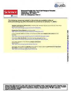
Figure 6: The performance ratio of Feedback-Rank versus Random (e.g., a of “2” value indicates that on average Feedback-Rank requires half of many false positives to be inspected to find the same number of bugs as Random). Results are for experiments when Feedback-Rank has none (Zero-Knowledge) and 25% (Partial-Knowledge) of the reports treated as being previously inspected.

5.1 Evaluating Ranking Performance We compare the performance of Feedback-Rank against Random by employing a scoring metric that summarizes ranking prowess over the entire inspection process. Recall that S(R) is the sum of the cumulative number of false positives inspected before each bug (see Equation 3 in Section 4.3). If we divide this quantity by N (the number of bugs), we get the average cumulative number of false positives inspected before each bug: Avg-FP = S(R)/N

(6)

This quantity measures the average inspection “delay” or “shift” per bug from Optimal. When we compare Feedback-Rank against Random, we simply take the ratio of Avg-FP for each ranking: Performance Ratio =

Avg-FP (Random) Avg-FP (Feedback-Rank)

(7)

This ratio is how many times more false positives on average we inspect before each bug using Random versus Feedback-Rank. For example if the ratio is 3 we inspect on average 3 times more false positives before each bug with Random than we do with Feedback-Rank.

5.2 What BN CPDs to Use? We require a BN model to apply Feedback-Rank to a set of reports. Construction of the BN structure follows the procedure outlined in Section 4.2, but to complete the model we need to specify the CPD values. The CPDs are learned from a set of inspected reports. For our experiments, we employ the following sets of CPDs: 1. Entire Codebase: We use CPDs trained on all the reports from a codebase. 2. Self-Trained: We use CPDs trained on the same set of reports that are being ranked 3. Reserved 90%: We reserve 90% of the reports from an error set, train the CPDs on that 90%, and rank the remaining reports using those CPDs. checking tools, they are quite willing to inspect a small set of the reports randomly if they can effectively use that labor to suppress the majority of the “problem spots” when inspecting the remaining reports.

We use the Entire Codebase CPDs when ranking reports from a different codebase. For example, when ranking reports from Linux we use the CPDs trained on System X. We can use the CPDs trained on a different codebase because we expect that the correlation trends based on code locality will generally hold across different checkers and codebases. For brevity, we will refer to this setup as Other Codebase. The first and second cases represent two practical extremes. The first case represents where we have no previous inspection data (or not enough) to tune the model to a specific checker/codebase. The second case represents what we can do with a fully tuned model (i.e., an “upper bound” on ranking performance). The third case is a realistic setup for using a tuned model, and we reserve it for our last experiment.

5.3 Results: Zero-Knowledge For the Zero-Knowledge experiment, we ranked the error sets in Table 1 using both Feedback-Rank and Random and compared the ranking results using Equation 7. Because the reports from a given checker are considered uninspected, we use the Other Codebase CPDs for our BN. In this experiment, we expected the largest improvement of Feedback-Rank over Random to come when there are (1) a fair number of reports and (2) strong clustering of false positives. For checkers with low false positive densities the improvement over Random should be marginal as both rankings are close to Optimal. The results, shown in the white bars in Figure 6, agree with our predictions. For most checkers we see at least a 50% improvement over Random, with checkers like Alock on Linux and Format on System X that have strong clustering of false positives having and improvement of 4x and 2x (respectively) over Random. The Free checker on Linux performs the same as Random because there are very few reports in total and little clustering, providing little correlation to exploit. On System X we observe for Rev-inull that Feedback-Rank performs marginally better than Random. This is because there is little clustering at the file and function level, and only occasional clustering at the directory level.

5.4 Results: Partial-Knowledge For the Partial-Knowledge experiment, we again individually ranked the reports from the checkers in Table 1, but this time randomly reserved 25% of the reports and treated them as being previously inspected. We then ranked the remaining reports using Feedback-Rank and Random.

Feedback-Rank vs. Random (Average # bugs found in N inspections)

Check

Bugs

FPs

Alock Block Free Intr Lock Null Param Range

7 122 10 20 12 92 8 53

29 13 5 37 37 35 10 2

5.4 10 6.9 7 5.9 8.2 6.1 10

N = 10

Exc-none Format Free Internal-null Inverse Lock Null Rev-inull

2 20 11 24 10 2 158 18

53 74 22 18 2 25 10 18

0.64 7.1 6.8 6.6 9.1 2 10 5.4

vs. vs. vs. vs. vs. vs. vs. vs. vs. vs. vs. vs. vs. vs. vs. vs.

1.9 8.9 6.7 3.4 2.3 7.2 4.5 9.6 0.44 2.1 3.4 5.7 8.3 0.78 9.5 4.9

N = 25 7 25

vs. vs.

4.8 23

N = 50 48

vs.

45

19

vs.

18

43

vs.

36

14 10 20

vs. vs.

8.7 6 18

25

vs.

24

48

vs.

48

2 9.7 10 17

vs.

1 5.3 8.7 14

2 17

vs. vs.

1.9 10

49

vs.

47

2 24 14

vs.

vs. vs. vs. vs. vs. vs.

1.8 24 12

Table 4: Average cumulative number of bugs found by Feedback-Rank and Random for the first 10, 25, and 50 inspections. Datasets are for the PartialKnowledge experiment (with Other Codebase BN model) with 25% of the reports previously inspected. Checkers from Linux are listed first.

reports (selected at random) from each checker. These are the reports generated by the checker tools on an “earlier” version of the codebase, while the remaining 10% are the “new” reports. Although we know there is cross-checker correlation between many of the checkers, we are still investigating how to best exploit it in our model. Instead of placing reports from all checkers within one BN, we compute probabilities by placing the reports from each checker in its own BN model, effectively treating reports from different checkers as independent. Reports from all checkers are then ranked together by their probabilities. For this experiment, we used the Reserved 90% CPDs for ranking. Figure 7 show our ranking results for System X. Depicted are the average cumulative number of bugs found after a given number of inspections for Optimal, Feedback-Rank, and Random. Both Feedback-Rank and Random are run 100 times, and error bars represent the region between the 5th and 95th percentile. For System X, Feedback-Rank is close to Optimal for the entire ranking, finding all 31 bugs after inspecting 3 (out of 28) false positives. For Linux (not shown), Feedback-Rank is always optimal for the first 14 inspections, and all 42 bugs are found after inspecting 9 (out of 21) false positives.

6. RELATED WORK

Figure 7: Ranking results for System X when reports from all checkers are ranked together (90% of reports reserved): 31 bugs, and 28 FPs

For Feedback-Rank we ranked the reports using both the Other Codebase CPDs and the Self-Trained CPDs. The performance ratios of Feedback-Rank versus Random for both CPD sets are shown in Figure 6. Table 4 also depicts the cumulative number of bugs found by both Feedback-Rank (using the Other Codebase CPDs) and Random for the first 10, 25, and 50 inspections. In many cases we see a dramatic improvement for Feedback-Rank over the results in the Zero-Knowledge experiment. From Figure 6 we see an average improvement of 2-3x over Random for the Other Codebase CPDs and an average improvement of 3-4x over Random for the Self-Trained CPDs. We see a factor of 6-8 improvement over Random for Alock (which finds 2.8 times as many bugs as Random for the first 10 inspections). Table 4 also shows that for Format Feedback-Rank finds 7 bugs in the first 10 inspections while Random finds only 2.

5.5 Results: Ranking Checkers Together Our final experiment estimates how useful Feedback-Rank would be as program checkers are continually applied to an evolving codebase. Because our error reports are from codebase snapshots, this is only a crude approximation. We simulate an evolving codebase by reserving 90% of the

There is significant interest in the program checking community in reducing false positive counts of tools. Both the PREfix and MC tools employ various rule-based ranking heuristics to identify the most reliable reports [4, 17]. Kremenek and Engler proposed z-ranking, a statistical ranking scheme that observes that error reports for code where an invariant often held and the tool flagged few errors in total are the most reliable [20]. Although these techniques are effective at suppressing false positives, they are static rankings that discard user feedback. Feedback-Rank is intended to complement these static ranking techniques to address this weakness. There has also been substantial effort on both dynamic and static techniques to better isolate defects. In the realm of dynamic tools, the problem is not with suppressing false positives, but identifying the source of a bug (which usually manifests as a program crash). In their system DIDUCE, Hangal and Lam track simple invariant properties and program values over the lifetime of an instrumented Java program [18]. They employ a ranking scheme to present to the user a list of tracked property values that were mostly consistent during the program’s execution but recently deviated before the crash. Liblit et al also dynamically track program state through statistical sampling to isolate crash causes. In a manner similar to ranking, for “non-deterministic” bugs where the exact cause cannot be easily isolated, they employ a logistic regression model to identify possible causes of crashes [21]. The coefficients of the model are used to identify the sampled program state values most correlated with the observance of the crash. For static tools, Ball et al looked at examining differences of paths traced by a modelchecker to isolate program points likely to be the root of a statically detected defect [2]. They looked primarily at isolating the cause of a bug, however, and are not addressing the issue of suppressing false positives. There has also been significant work at looking at empirical bug densities in systems and how bugs cluster. Chou

et al studied the lifetimes and densities of bugs found in open-source operating system code by the MC system, and Ostrand et al studied the densities of faults discovered by testing during the entire development lifetime of a large commercial software project [6, 22]. Chou observed that bugs frequently cluster by checked invariant and code locality; in device driver code error rates were up to 7 times larger than other sections of the code base. Ostrand observed a significant positive correlation between code that was fault prone in a previous release and the likelihood it was fault prone in a subsequent release of the project. Although he employs software testing data, we expect bugs found by static tools to similarly correlate, as it is a characteristic property of the code itself. Moreover, we expect false positives to correlate over a project’s lifetime. Unless the checking tool is fixed, “problem spots” that caused the tool to make analysis mistakes will remain in the code unless the code is significantly rewritten or the tool fixed.

7.

CONCLUSION

This paper presented Feedback-Rank, an on-line ranking algorithm for inspecting error reports emitted by static checking tools. It operates on the simple premise of associating with each report a probability that it is a true error and then sorts reports by their probabilities. After each inspection, the probabilities for the remaining reports are updated by using a probabilistic model. Our main source of leverage was that reports frequently correlate by code locality, but there are many potential sources of correlation to exploit. Another possible source of correlation is for code that implements a common interface (e.g., device drivers). If a checking tool reveals that a particularly implementation is buggy, other flagged errors for related implementations may also be real bugs because of similar idiomatic problems. Code versioning information may also be a potentially rich source of data for correlating reports, as code written by the same developer may have correlated bug densities and code written at the same time may also be highly correlated in the same manner. There are many other ways in which reports can be correlated, and potentially exploited for ranking. Feedback-Rank represents a complementary approach to static ranking schemes. Static schemes can be used to perform an initial sorting, while Feedback-Rank can be used to adaptively alter the ranking as feedback is introduced. In practice our ranking strategy works well, and without having any knowledge of the internals of the code checked or the analysis algorithms used. We observed a factor of 2-8 improvement over randomized ranking, and when some previous error report data was available it frequently performed close to optimal on the first several inspections.

8.

ACKNOWLEDGEMENTS

We thank Godmar Back, David Yu Chen, Chris Lattner, Ben Liblit, Andrew Ng, Paul Twohey, Chris Unkel, and the anonymous reviewers of this paper for their many insightful and valuable comments. This research was supported by DARPA grant F29601-01-2-0085.

9.

REFERENCES

[1] A. Aiken, M. Faehndrich, and Z. Su. Detecting races in relay ladder logic programs. In TACAS 1998, 1998.

[2] T. Ball, M. Naik, and S. K. Rajamani. From symptom to cause: localizing errors in counterexample traces. In POPL 2003, 2003. [3] T. Ball and S. Rajamani. Automatically validating temporal safety properties of interfaces. In SPIN 2001 Workshop on Model Checking of Software, May 2001. [4] W. Bush, J. Pincus, and D. Sielaff. A static analyzer for finding dynamic programming errors. Software: Practice and Experience, 30(7):775–802, 2000. [5] H. Chen and D. Wagner. MOPS: an infrastructure for examining security properties of software. In Proceedings of the 9th ACM conference on Computer and communications security, pages 235 – 244. ACM Press, 2002. [6] A. Chou, J. Yang, B. Chelf, S. Hallem, and D. Engler. An empirical study of operating systems errors. In SOSP 2001. [7] T. M. Cover and J. A. Thomas. Elements of Information Theory. Wiley Interscience, 1991. [8] R. G. Cowell, A. P. Dawid, S. L. Lauritzen, and D. J. Spiegelhalter. Probabilistic Networks and Expert Systems. Springer, 1999. [9] M. Das, S. Lerner, and M. Seigle. Path-sensitive program verification in polynomial time. In PLDI 2002, 2002. [10] D. Engler, B. Chelf, A. Chou, and S. Hallem. Checking system rules using system-specific, programmer-written compiler extensions. In OSDI 2000, 2000. [11] D. Evans, J. Guttag, J. Horning, and Y. Tan. LCLint: A tool for using specifications to check code. In FSE 1994, 1994. [12] D. Evans and D. Larochelle. Improving security using extensible lightweight static analysis. IEEE Software, 19(1):42–51, January/February 2002. [13] C. Flanagan and S. N. Freund. Type-based race detection for Java. In PLDI 2000, 2000. [14] C. Flanagan, K. Leino, M. Lillibridge, G. Nelson, J. Saxe, and R. Stata. Extended static checking for Java. In PLDI 2002, pages 234–245. ACM Press, 2002. [15] J. Foster, T. Terauchi, and A. Aiken. Flow-sensitive type qualifiers. In PLDI 2002, 2002. [16] P. Good. Permutation Tests: A Practical Guide to Resampling Methods for Testing Hypotheses. Springer, 2000. [17] S. Hallem, B. Chelf, Y. Xie, and D. Engler. A system and language for building system-specific, static analyses. In PLDI 2002, 2002. [18] S. Hangal and M. S. Lam. Tracking down software bugs using automatic anomaly detection. In International Conference on Software Engineering, May 2002. [19] Intrinsa. A technical introduction to PREfix/Enterprise. Technical report, Intrinsa Corporation, 1998. [20] T. Kremenek and D. Engler. Z-Ranking: Using statistical analysis to counter the impact of static analysis approximations. In SAS 2003, 2003. [21] B. Liblit, A. Aiken, A. X. Zheng, and M. I. Jordan. Bug isolation via remote program sampling. In PLDI 2003, 2003. [22] T. J. Ostrand, E. J. Weyuker, and R. M. Bell. Where the bugs are. In ISSTA 2004, 2004. [23] U. Shankar, K. Talwar, J. S. Foster, and D. Wagner. Detecting format string vulnerabilities with type qualifiers. In Proceedings of the 10th USENIX Security Symposium, 2001. [24] D. Wagner, J. Foster, E. Brewer, and A. Aiken. A first step towards automated detection of buffer overrun vulnerabilities. In 2000 NDSSC, Feb. 2000. [25] J. S. Yedidia, W. T. Freeman, and Y. Weiss. Understanding belief propagation and its generalizations. In Exploring Artificial Intelligence in the New Millennium, pages 239–269. Morgan Kaufmann Publishers Inc., 2003.