Sep 22, 2004 - arbitrary age, not only a first principle derivation is miss- ing, a condition ...... [17] P. Allegrini, P. Grigolini, L. Palatella, A. Rosa, B. J.. West, in ...
Correlation function and generalized master equation of arbitrary age Paolo Allegrini1 , Gerardo Aquino2 , Paolo Grigolini2,3,4, Luigi Palatella5 , Angelo Rosa6 and Bruce J. West7 1 INFM, unit` a di Como, Via Valleggio 11, 22100 Como, Italy Center for Nonlinear Science, University of North Texas, P.O. Box 311427, Denton, Texas 76203-1427 3 Dipartimento di Fisica dell’Universit` a di Pisa and INFM, Via Buonarroti 2, 56127 Pisa, Italy 4 Istituto dei Processi Chimico Fisici del CNR Area della Ricerca di Pisa, Via G. Moruzzi 1, 56124 Pisa, Italy 5 Istituto dei Sistemi Complessi del CNR, P.le A. Moro 2, 00185 Rome, Italy 6 Institut de Math´ematiques B, Facult´e des Sciences de Base, ´ Ecole Polytechique F´ed´erale de Lausanne, 1015 Lausanne, Switzerland and 7 Mathematics Division, Army Research Office, Research Triangle Park, NC 27709, USA
arXiv:cond-mat/0409600v1 [cond-mat.stat-mech] 22 Sep 2004
2
We study a two-state statistical process with a non-Poisson distribution of sojourn times. In accordance with earlier work, we find that this process is characterized by aging and we study three different ways to define the correlation function of arbitrary age of the corresponding dichotomous fluctuation. These three methods yields exact expressions, thus coinciding with the recent result by Godr`eche and Luck [J. Stat. Phys. 104, 489 (2001)]. The first method rests on the lines established in an earlier paper [Allegrini et al., Phys. Rev. E 68, 056123]. These authors built up an infinitely aged Generalized Master Equation (GME), compatible with the ordinary Onsager Principle. Herein we generate first a GME of arbitrary age, then we derive from it an expression for the corresponding correlation function, based on the Onsager principle extended to a condition of generic age. To derive the second exact expression of correlation function of arbitrary age, we use a Liouville-like approach, based on a model mimicking the environment responsible for the fluctuations of the dichotomous variable under study, and producing the same non-Poisson distribution of sojourn times as that considered in the earlier treatment. This exact expression refers to time t, while the earlier exact expression refers to the variable u, which is the Laplace conjugate of t. Finally, the third exact expression, again with respect to time, is derived from the direct observation of the dichotomous sequence generated by the two-state system fluctuations. The resulting expression is implicit, and we adopt a convenient approximation to obtain a simple analytical formula. This approximation rests on the renewal nature of the process, which resets to zero the memory of the system after the occurrence of any event, thereby suggesting that a Markovian approximation can be made. Actually, non-Poisson statistics yields infinite memory at the probability level, thereby breaking any form of Markovian approximation, including the one adopted herein. For this reason, we check the accuracy of the analytical formula by comparing it with the numerical treatment of the second of the three exact expressions. We find that, although not exact, the simple analytical expression for the correlation function of arbitrary age is very accurate. PACS numbers: 02.50.Ey, 05.40.Fb, 05.20.-y, 05.60.Cd
I.
INTRODUCTION
The phenomenon of aging has been known for a long time as a property of spin glasses and polymers [1]. Part of the reason for the more recent interest in this phenomenon has to do with the predicted breakdown of certain fundamental assumptions made in equilibrium statistical mechanics when applied to strongly disordered systems. For example, the Onsager Principle [2], being the relaxation of a perturbed system back to its equilibrium state as described by an unperturbed autocorrelation function, is violated in anomalous diffusion and anomalous relaxation. More recent papers on this phenomenon are devoted to studying aging in diffusion processes occuring in d-dimensional lattices [3], in low dimensional environments [4] and in the quantum dynamics of dissipative free particles [5]. Most recently [6, 7] there has been some interest in the manifestation of aging in processes described by means of the Continuous Time Random Walk (CTRW) formalism [8]. A natural way of formally expressing aging is through
the correlation function of the stochastic variable of interest, ξ, which is expressed as an ensemble average indicated by the brackets hξ(t1 )ξ(t2 )ita (t ) ≡ Φξ a (t1 − t2 ). hξ 2 i
(1)
The averaging brackets carry a subscript stressing that this is a ta -old property, rather than the traditional aged property, only depending on |t1 − t2 |. The time difference indicates the stationarity of the underlying process, but the ta -superscript denotes a dependence on the age of the process as well. In the case of a dichotomous variable obeying renewal theory, the exact expression for the Laplace transform of this age-dependent correlation function was found by Godr`eche and Luck [9]. Their exact result was recently recovered by Margolin and Barkai [10] as a special case of a more general expression, since the latter authors do not require the condition that the two states of the dichotomous variable ξ have the same waiting-time distribution. However, herein we make the same assumption as did Godr`eche and Luck [9], and de-
2 rive their result along the lines of the recent work of Ref. [7]. Allegrini et al. [7] noticed that in the non-Poisson case the well known Generalized Master Equation (GME) of Kenkre, Montroll and Shlesinger [11] becomes incompatible with the Onsager principle [2] and found a way to make the GME compatible with the aged condition. However, they [7] left unsolved the problem of deriving a GME of arbitrary age, which is equivalent to making the Onsager principle compatible with an incompletely aged system. Here we solve this problem and establish that this solution leads to the exact expression for the correlation function of arbitrary age found by Godr`eche and Luck [9]. The GME derived herein does not have the same origin as those widely discussed in the literature [12]. The Zwanzig GME, in fact, one of the most popular master equations, is derived from a first principles procedure, starting from the statistical Liouville equation of the whole universe. The Zwanzig GME is a projection of this universal Liouville equation onto the Hilbert space of the system of interest. The approach used to derive the GME herein is quite different from that of Zwanzig and is based on the experimental observation of non-Poisson dichotomous signals. Examples of such signals include those produced by an ionic channel [13] and by blinking quantum dots [14]. We build up a GME that is compatible with the experimentally determined non-Poisson nature of these processes, assuming the applicability of renewal theory. We leave open the question as to the source of randomness, but note in passing that the fluctuations in the system variable are generated by the environment. A simplified dynamical model has reproduced the essential statistical properties of the system of interest, in the case of infinitely aged GME [15]. In the case of arbitrary age, not only a first principle derivation is missing, a condition shared by the infinitely aged case: there is, to date, not even a heuristic derivation derivation of the corresponding GME. Herein we provide a heuristic derivation of a GME with arbitrary age, one based on an exact expression for the corresponding distribution of sojourn time, and we use this result to derive an exact expression for the correlation function. In conclusion, we point out that we rework the problem from a number of perspectives. We do this because each approach provides separate and distinct insights into the phenomenon described by a GME of arbitrary age. The first perspective adopted in this paper focuses on the derivation of a GME, based on the experimental observation of the time evolution of a trajectory, characterized by rare jumps from one state to another. The second perspective uses a Liouville-like approach to the time evolution of the variable of interest and its environment. No attempt is made to derive the former dynamic picture (trajectory) from the latter (probability density). The probability density perspective is characterized by infinite memory, yet, the statistical process under study is generated by random critical events, whose occurrence erases the memory of earlier events. Therefore, we think
it is prudent to examine, yet again, the same process from a third perspective, one based on the direct observation of the sequence of rare random events. We find that the use of three different perspectives is fruitful in shedding light on the recent observation made by Sokolov, Blumen and Klafter [16]. Their results, in our opinion, imply the breakdown of certain well-established notions of equilibrium statistical mechanics, such as linear response theory as a prescription for predicting the effect of externally perturbing a system out of equilibrium. The outline of the paper is as follows. In Section II we employ the reduced density perspective, namely, we build up the GME of arbitrary age. In Section III we study the time evolution of the total distribution density. In Section IV we use a third method, based on the probability of occurrence of the rare random events. Section V is devoted to concluding remarks.
II.
THE REDUCED DENSITY PERSPECTIVE
This section is devoted to the application of the reduced density perspective to the construction of the GME. In the literature of statistical physics this perspective implies a contraction on the total density onto a prescribed subspace. Consequently, constructing the equation of motion of the total density matrix should be the first step. The reason why we reverse the perspective, thereby confining the total density treatment to the next section is given by the fact that non-Poisson statistics has the effect of making the ordinary approach extremely difficult, if not impossible, as discussed in the companion papers [15, 17]. The derivation of the GME is made possible by expressing the higher-order correlation functions in terms of the second-order correlation function, via simple expressions that are violated by the Poisson statistics. This is the reason why we derive the GME from the Continuous Time Random Walk (CTRW) of Montroll and Weiss [8, 18], rather than from the equation of motion for the total distribution density.
A.
From the generalized master equation to the age-dependent correlation function
The reduced density matrix perspective is based on the adoption of the GME formally defined by d p(t) = − dt
Z
t
Φ(t − t′ )Kp(t′ )dt′ ,
(2)
0
where p (t) is the m-dimensional population vector of m sites, so that its ith component, pi (t), represents the probability of finding the walker at time t in the ith site. K is a transition matrix between the sites and Φ(t) is the memory kernel. We study the case where the fluctuating variable ξ leading to this GME is dichotomous. This
3 means that the GME has only two states and the matrix K reads
K=
�
1 −1 −1 1
�
.
(3)
The waiting-time distribution in either of the two states is denoted by ψ(t). We establish the connection of the GME with the CTRW [7, 8] by relating the Laplace transform ˆ of the memory kernel Φ(t), given by Φ(u), to the Laplace transform of the waiting-time distribution ψ(t), given by ˆ ψ(u), as follows ˆ uψ(u) ˆ . Φ(u) = ˆ 1 − ψ(u)
(4)
We consider two distinct processes, that of preparation and that of observation. The preparation process establishes the initial conditions of the set of trajectories under study. A trajectory is a sequence of symbols + or −, specifying whether the system is in the state |+i or |−i. We call the time interval with the system either entirely in the state |+i or entirely in the state |−i, the laminar region. With Zumofen and Klafter [19], we assume that the preparation process, beginning at time t = −ta , insures that all these trajectories begin with the system at the onset of a laminar region, either + or −. The observation process begins at time t = 0 ≥ −ta . The distribution of first sojourn times is denoted by ψta (t) and is, in general, different from ψ(t). In fact, the laminar region corresponding to the first sojourn time might have begun earlier than t = 0. The exact expression for this time distribution is ∞ Z ta X dyψ(y + t)ψn (ta − y), (5) ψta (t) = ψ(t + ta ) + n=1
In the Poisson case, because of its unique functional form, there is no dependence of ψta on ta , and consequently no aging. In the non-Poisson case, on the contrary, the two waiting-time distributions, ψta and ψ(t), are identical only if ta = 0. In this case both CTRW and GME correspond to switching-on the observation process at the same time as the preparation process, and the connection between the two pictures is given by Eq. (4). Allegrini et al. [7] proved that the GME is compatible with an infinitely aged CTRW, provided that the memory kernel Φ(t) is made compatible with an infinitely aged condition, characterized by a distribution of first sojourn times, which is infinitely aged. In this case ta → ∞ so that
0
where ψn (τ ) denotes the probability that n jumps occur during the time interval of length τ , the last of which occurs at time t = τ . As is well known, for a renewal process the waiting times for successively more jumps is given by the convolution Z t ψn (t) = ψn−1 (t′ )ψ1 (t − t′ )dt′ , (6) 0
with ψ(t) ≡ ψ1 (t). The ta -old distribution of first sojourn time was discussed earlier in some detail [20]. However, a careful analysis of Eq. (5) can help the reader to realize the rationale behind this distribution of sojourn times. The first term on the right hand side of Eq. (5) corresponds to the case when the first laminar region is extended in time more than the time interval ta between preparation and observation. The second term takes into account the cases when the last laminar region began after the preparation time, after a sequence of an arbitrarily large number of earlier laminar regions, the first of which, of course, begins at t = −ta .
ˆ ∞ (u) = Φ
uψˆ∞ (u) , ˆ 1 + ψ(u) − 2ψˆ∞ (u)
(7)
where 1 ψ∞ (t) = hτ i
Z
∞
dt′ ψ(t′ ).
(8)
t
It is straigthforward to extend the calculations of Ref. [7] to the case of an arbitrarily ta -old system, so that Eq.(7) is replaced with ˆ ta (u) = Φ
uψˆta (u) , ˆ 1 + ψ(u) − 2ψˆta (u)
(9)
where ψˆta (u) is the Laplace transform of ψta (t). Using the GME with the ta -old memory kernel, we (t ) define the age-dependent correlation function Φξ a (t) through its Laplace transform, as follows ˆ (ta ) (u) = Φ ξ
1 . ˆ ta (u) u + 2Φ
(10)
This prescription corresponds to setting (t )
Φξ a (t) =
p1 (t) − p2 (t) , p1 (0) − p2 (0)
(11)
as one can easily check by Laplace transforming both sides and using the GME with the ta -old memory kernel (see section II B). In other words, the correlation function of arbitrary age mirrors the extension of the Onsager principle, which is usually limited to infinitely aged systems [7], to physical conditions of arbitrary age. It has to be pointed out that at this stage there is no guarantee that the Onsager principle of arbitrary age holds true. However, in Section II B we show that Eq. (10) yields the exact result of Godr`eche and Luck [9] for the corresponding correlation function. Furthermore, in Section II C we establish the same result using arguments based on trajectories rather than densities, thereby affording an independent construction of the exact expression for the ta -old correlation function. All this can be thought of as a compelling demonstration of the correctness of of Eq. (11), extending the Onsager principle to conditions of arbitrary age.
4 B. Derivation of the exact expression proposed by Godr` eche and Luck: the probability perspective
To establish that the proposed approach yields the exact expression of Godr`eche and Luck [9], let us express the ta -old correlation function through the probability vector p ≡ (p1 , p2 ) for the dichotomous variable ξ = ±1 to have either positive (state 1) or negative (state 2) values. We have that: hξ(0)ξ(t)ita (t ) = (12) Φξ a (t) = hξ 2 i p1 (0)p1 (t|1, t = 0) + p2 (0)p2 (t|2, t = 0) −p1 (0)p2 (t|1, t = 0) − p2 (0)p1 (t|2, t = 0), where pj (t|k, t = 0) is the conditional probability that the variable ξ is in the state j at time t, given that at time t = 0 it was in the state k. This means that pj (t|k, t = 0) is obtained letting those trajectories evolve that at time t = 0 had ξ in the state k. For a straightforward evaluation of pj (t|k, t = 0), we use the GME formalism, adapted to the ta -old system, and we take into account the initial condition pi (0|k, t = 0) = δi,k . According to the GME the components of the conditional probability vector are determined by: Z t 2 X d Kji pi (t′ |k, t = 0), pj (t|k, t = 0) = − dt′ Φta (t−t′ ) dt 0 i=1 (13) ˆ ta (u) given by Eq. (9) and the elements of K given with Φ by Eq. (3). By Laplace transforming (13) and doing some algebra, we obtain pˆj (u|k, 0) =
2 X
ˆ ta (u)K)−1 pi (0|k, 0). (uI + Φ ji
(14)
i=1
We note that the probability is normalized, p1 (0) + p2 (0) = 1. Thus, it follows that ˆ ˆ ˆ (ta ) (u) = �u + Φta (u) � − � Φta (u) � [p1 (0) Φ ξ ˆ ta (u) ˆ ta (u) u u + 2Φ u u + 2Φ +p2 (0)] =
1 , ˆ ta (u) u + 2Φ
(17) confirming the correctness of the definition introduced in Eq. (10). Substituting (9) into (17) we obtain # " 1 1 2ψˆta (u) (ta ) ˆ i= , Φξ (u) = h 1− ˆt (u) ψ ˆ u a 1 + ψ(u) u 1 + 2 1+ψ(u)−2 ˆ ˆ ψ (u) ta
(18) which coincides with the results of Godr`eche and Luck [9]. Furthermore, the ratio of the differences in probability is determined in Laplace space by 2 X (J1i − J2i )pi (0) pˆ1 (u) − pˆ2 (u) = p1 (0) − p2 (0) p1 (0) − p2 (0) i=1
=
1
ˆ ta (u) u + 2Φ
(19)
(t )
ˆ a (u). =Φ ξ
As pointed out earlier, Eq.(19) means that one can extend the Onsager Principle from the infinitely aged systems, for which Onsager originally defined it, to systems of any age. In the latter case the relaxation is proportional to the ta -old correlation function, not to the infinitely old, or equilibrium, correlation function. In summary, we discovered an Onsager principle of arbitrary age, at least in the special case of the dichotomous variables considered in this paper.
Defining the matrix
ˆ ta (u)K)−1 = J = (uI+ Φ
ˆ t (u) u+Φ a ˆ t (u)] u[u+2Φ a ˆ t (u) Φ a ˆ t (u)] u[u+2Φ a
ˆ t (u) Φ a ˆ t (u)] u[u+2Φ a ˆ t (u) u+Φ a ˆ t (u)] u[u+2Φ a
,
and using the initial condition pi (0|k, t = 0) = δi,k , we obtain for the Laplace transform of the conditional probability vector the following expression i h ˆ ta (u) (δj,k+1 + δj,k−1 ) ˆ ta (u) δj,k + Φ u+Φ i h . pˆj (u|k, 0) = ˆ ta (u) u u + 2Φ
(15) Using Eq. (15) we can Laplace trasform (12) to obtain ˆ ˆ ˆ (ta ) (u) = p1 (0) �u + Φta (u) � + p2 (0) �u + Φta (u) � Φ ξ ˆ ta (u) ˆ ta (u) u u + 2Φ u u + 2Φ ˆ (u) ˆ ta (u) Φ Φ � − p2 (0) � ta � − p1 (0) � ˆ ta (u) ˆ ta (u) u u + 2Φ u u + 2Φ (16)
C. Derivation of the exact expression proposed by Godr` eche and Luck: the trajectory perspective
It is possible to again derive the exact result of Eq. (18) from a different perspective, which will allow us, in Section IV, to propose an analytic expression for the ta -old correlation function as a function of time. This expression, as we shall see, is not exact, but it is shown numerically to be a very good approximation to the exact result. The usual method of connecting the correlation function Φξ to the waiting-time distribution, within a trajectory perspective, is to introduce a theoretical waitingtime distribution, ψ ∗ (t), which cannot be observed directly. In fact, the experimental waiting-time distribution, namely, the distribution of times with alternate signs, denoted by us as ψ(t), is obtained from the theoretical waiting-time distribution, ψ ∗ (t), by adopting the following procedure. We divide the time axis into bins, whose size is determined by the waiting-time distribution
5 ψ ∗ (t). Then, these bins are assigned either the value 1 or the value −1, by tossing a coin to make the decision. It is evident that the intervals along the time axis with the same sign, are larger than the time bins determined by ψ ∗ (t), since two or more consecutive coin tossings might have produced the same sign. It is shown [19] that the Laplace transform of ψ is connected to the Laplace transform of ψ ∗ via the relation ˆ ψ(u) =
ψˆ∗ (u) . 2 − ψˆ∗ (u)
(20)
Let us use the term event to denote the coin tossing introduced above. The expression (20) is the result of summing over all possibilities of not changing sign with a coin toss, which turns out to be a geometrical series in the Laplace representation. The correlation function Φξ and the theoretical waiting-time distribution function ψ ∗ are connected through the relation R∞ (t − τ )ψ ∗ (τ )dτ , (21) Φξ (t) = t hτ i where the average waiting time is given by Z ∞ hτ i ≡ τ ψ ∗ (τ )dτ.
(22)
0
Eq. (21) determines that the correlation function Φξ (t) is equal to the probability of finding a window of length t without internal events. The same result can be immediately recovered using Z ∞ ∗ dt′ ψ∞ (t′ ) (23) Φξ (t) = Ψ∗∞ (t) ≡ t Z ∞ Z ∞ 1 = dt′ dt′′ ψ ∗ (t′′ ). hτ i t t′ We note that, see Ref. [7], ∗ ψ∞ (t)
1 ≡ hτ i
Z
ψˆta (u) =
ψˆt∗a (u) . 2 − ψˆ∗ (u)
(27)
Using Eq. (20) we write Eq. (27) as 2ψˆta (u) . ψˆt∗a (u) = ˆ 1 + ψ(u)
(28)
By Laplace transforming Eq. (25) and using Eq. (28), we obtain " # 1 − ψˆt∗a (u) 2ψˆta (u) 1 (ta ) ˆ 1− = Φξ (u) = , (29) ˆ u u 1 + ψ(u) namely, we again recover the exact result of Godr`eche and Luck given by Eq. (18). This establishes the equivalence of the trajectory and GME prescriptions for this process. D.
Generalized Master Equation of arbitrary age
We are now in a position to make a preliminary balance of the results obtained so far. The first is that we have generalized the result of an earlier paper [7], in that we have derived the GME of arbitrary age
∞
dt′ ψ ∗ (t′ )
(24)
d p(t) = − dt
t
is the infinitely aged waiting-time distribution. Actually, Eq. (23) is the infinitely aged correlation function, a special case of the more general prescription Z t Z ∞ (t ) dt′ ψt∗a (t′ ). dt′ ψt∗a (t′ ) = 1 − Φξ a (t) = Ψ∗ta (t) ≡ t
where the symbol ⋆ denotes time convolution. In fact, after a first interval of time followed by a coin toss with no change of sign, determined by ψt∗a /2, the next intervals of time with no change of sign according to the coin tossing prescription, are determined by ψ ∗ /2. The sum of the convolutions takes into account all the possible sequences of intervals of time with no change of sign before a change of sign of the variable ξ eventually occurs, and gives as final result the distribution for a first observed sojourn time t of the variable ξ in one of its two states, that is ψta (t). Thus by summing the geometric series in the Laplace variables, from (26) we obtain
0
(25) It is straightforward to show that the ta -old experimental waiting-time distribution and the ta -old theoretical waiting-time distribution are connected through the following sum of convolutions: � 1 1 ∗ (26) ψta (t) = ψta (t) ⋆ δ(t) + ψ ∗ (t) 2 2 � 1 1 + ψ ∗ (t) ⋆ ψ ∗ (t) + · · · , 2 2
Z
t
Φta (t − t′ )Kp(t′ )dt′ ,
(30)
0
whose memory kernel Φta (t) is defined though its Laplace transform by means of Eq. (9). We have also shown that the Onsager principle, valid for infinitely aged systems, can be extended to conditions of any age, and that this extension allows us to derive an exact expression for the ta -old correlation function. However, the analytic results obtained so far are in the Laplace domain. It is desireable to achieve them in the time domain, as well. We now turn our attention to the latter. III.
THE LIOUVILLE-LIKE APPROACH
In this section we derive another expression for the ta -old correlation function adopting a perspective where
6 aging is determined by the out of equilibrium bath for the variable of interest, ξ. There might exist conditions, as we shall see, where equilibrium is not even allowed. The expression for the ta -old correlation function afforded by this perspective is exact, and is thus equivalent to the Godr`eche and Luck expression of Eq. (18). However, the exact expression is implicit, rather than explicit, and is therefore more convenient for the numerical calculations done subsequently. Here we adopt the perspective of earlier work [17, 21] to account for the aging effects characterizing the fluctuations of the dichotomous variable ξ. These fluctuations occur while the environment of the variable, ξ, slowly drifts. This drifting process is extended over time, and could lead to circumstances where it is not possible to attain equilibrium asymptotically. In keeping with the jargon of statistical mechanics the environmental or “irrelevant” variable is called y and in the model moves in the interval I = [0, 2]. In the semi-interval [0, 1], we use the equation of motion for the probability density ∂p(y, t) ∂ = −λ y z p(y, t), ∂t ∂y
(31)
This is the motion determined by a potential, with the minimum at y = 1, in the over-damped case. In the interval [1, 2], the over-damped potential is the mirror image of the potential acting on the left interval. Consequently, if the initial condition is located in the internal part of the interval [0, 1], the particle moves, from the left to the right, with a deterministic motion, towards y = 1. If the particle is initially located in the interior of the interval [1, 2], it moves deterministically from the right to the left. When the particle reaches the potential minimum, it is injected back, with equal probability, into any of the points of the interval I excluding y = 0, y = 1 and y = 2. The time spent by y within I corresponds to sojourning in one of the two states of the variable ξ, either |+i or |−i. The instant of back injection corresponds to the choice of the new state and, with equal probability, this is either the same state or the other state. The variable y represents the environment of the variable ξ, and its initial distribution is given by the state of the bath. The corresponding waiting-time distribution between two consecutive back injections is ψ ∗ (t) = (µ − 1)
T µ−1 , (t + T )µ
(32)
where the index µ is related to z of Eq. (31) by z , (33) µ≡ z−1 and the parameter T , characterizing the waiting-time distribution of Eq. (32) is µ−1 , (34) λ in accordance with the normalization constraint. The authors of Refs. [7, 15] have shown that the essential properties of the dichotomous non-Poisson fluctuation can be T ≡
accounted for by limiting ourselves to this simplified picture, involving only the semi-interval [0, 1]. In this simple picture the aging process is described by ∂ ∂p(y, t) = −λ y z p(y, t) + λp(1, t), ∂t ∂y
(35)
which takes into account the back injection into the semiinterval, occurring with uniform probability, when the particle reaches the point y = 1. For simplicity, but with no loss of generality, we fix λ = 1. Using the results of Ref. [17] the ta -old correlation function is evaluated as follows. The bath is prepared at time t = −ta . This means that at time t = −ta the distribution of y within the interval I is flat. In the case z < 2 this distribution tends to the equilibrium distri1 bution, peq ∝ yz−1 . If z > 2 this distribution diverges, thereby implying that the distribution approaches the Dirac delta function located at y = 0. This is the nonstationary condition, the condition where equilibrium is not allowed, and only a condition of eternal drift is admitted. Suppose this distribution evolve for a time ta , without our observing it. This means that we begin the observation process when the system has a new distribution, different from the initial flat distribution, and determined by its time evolution from t = −ta to t = 0, described by Eq. (35). For t ≥ 0 Eq. (35) is replaced with Eq. (31) ∂ ∂p(y, t) = − y z p(y, t), ∂t ∂y
(36)
namely the back injection process is stopped, thereby implying that the population decreases. The theory of Ref. [17] relates the probability solution to the Liouville-like equation to the ta -old correlation function as follows Z 1 (ta ) Φξ (t) = dyp(y, t). (37) 0
Note that the initial condition p(y, 0) is obtained from Eq. (35) moving from the flat distribution at t = −ta . The time evolution, corresponding to the observation process, is determined by Eq. (36). This simple picture is a fair representation of the description made in terms of trajectories in Section II. The fact that the norm of p(y, t), when p(y, t) is described by Eq. (36), is not conserved, reflects the occurrence of jumps from one state to the other, making the population of a given state decrease. Let us remark that the correlation function is determined by the antisymmetric part of the whole distribution [17]. This formal condition corresponds to observing the time evolution of p(y, t), with y ranging from y = 0 to y = 1, under the action of Eq.(31), with no back injection process. The process of back injection is essential to determine the correlation function of arbitrary age. However, once the parameter ta is fixed, and with it the age of the correlation function, the evaluation of the correlation function is done by imagining the bath frozen
7 in the distribution corresponding to this fixed age. This is the reason we use Eq. (31) to determine the correlation function rather than Eq. (35). The process of back injection is essential for the slow environmental drift, but the correlation time of age ta is determined by the age-fixed condition, the bath being ta -old, and keeping this age forever. Our goal is to calculate the correlation function of arbitrary age. According to Eq. (37), this goal requires that we evaluate p(y, t), first. To carry out this calculation we follow the procedure illustrated in detail in Ref. [22]. The time evolution from t = −ta to t < 0 is described by Eq. (35), yielding for the solution 1 (38) [1 + (z − 1)(t + ta )y z−1 ]z/(z−1) Z t p(1, τ )dτ + , z−1 ]z/(z−1) −ta [1 + (z − 1)(t − τ )y
p(y, t) =
with p(1, τ ) determined, in turn, by Eq. (35). As already stated, for t > 0, p(y, t) is governed by Eq. (36), so that its solution is, given the initial value, p(η, 0) y |η= [1+(z−1)yz−1 t]1/(z−1) [1 + (z − 1)y z−1 t]z/(z−1) (39) Now, we can calculate the final expression for the agedependent correlation function given by Eq. (37). After some simple algebra we obtain the following expression: p(y, t) =
(t )
Φξ a (t) = + = = + −
1 (40) [1 + (z − 1)(t + ta )]1/(z−1) Z 0 p(1, τ )dτ 1/(z−1) −ta [1 + (z − 1)(t − τ )] Z 0 p(1, τ )dτ Ψ∗ (t + ta ) + [1 + (z − 1)(t − τ )]1/(z−1) −ta Ψ∗ (t + ta ) + [1 − Ψ∗ (ta )] Z 0 p(1, τ )dτ [1 + (z − 1)(t − τ )]1/(z−1) −ta Z 0 p(1, τ )dτ . [1 − (z − 1)τ ]1/(z−1) −ta
Note that in Eq.(40) we are using the definition ∗
Ψ (t) =
Z
• if the age vanishes ta → 0, then the ta -old correlation function reduces to the probability of no event (t ) occuring Φξ a (t) → Ψ∗ (t). • if the age increases without limit ta → ∞, then the ta -old correlation function reduces to a known (t ) result Φξ a (t) → Φξ (t), where Φξ (t) =
1 [1 + (z − 1)t](2−z)/(z−1)
(42)
is the usual correlation function calculated at equilibrium. So, we must observe a crossover between two distinct regimes. Moreover, we anticipate that we recover these results from a different perspective in Sec. IV. The perspective adopted in this section makes it easier to understand, on physical grounds, why the Poisson condition produces aging. The Poisson condition corresponds to z = 1 in the nonlinear dynamical map, and in this case the distribution is always flat. Aging is the process of slow regression of the bath variable to equilibrium, a process that can, in principle, last forever. With this representation it is possible to study the correlation function of arbitrary age also in the case µ < 2. Allegrini et al. [17] give a detailed discussion of the effect of external perturbations. In the case z < 2 equilibrium is possible. An external perturbation can be used to create a condition whereby the system is out of equilbrium. The observation of the population difference between the two states, ξ = 1 and ξ = −1, is equivalent to determining the correlation function. Note that the initial condition that we use to study the time evolution of p(y, t) during the observation process, Eq. (36), is the antisymmetric distribution of the interval [0, 2] folded into [0, 1] (see Ref. [17]). It is evident that in practice the equilibrium correlation function is never observed. In fact, the external perturbation should create a non-symmetric initial condition in the whole interval [0, 2]. The anti-symmetric portion of this distribution, folded into the interval [0,1], should create the same out of equilibrium distribution as that produced by folding in the same way the anti-symmetric portion of the equilibrium distribution. As pointed out in Ref. [17], this is impossible to do in practice with a a perturbation lasting for a finite time, and, thus, with any realistic experimental procedure.
∞
ψ ∗ (τ )dτ.
(41)
t
This notation for the survival probability is also used in Section IV A. We notice that, t > 0 and p(1, t) is calculated from Eq. (35) with y = 1 and −ta < t < 0. This is an exact expression that turns out to be convenient to numerically check the prescriptions of Section IV. It is worth using the perspective of this section to shed further light into the problem under discussion in this paper. Let us notice that
IV. AN ANALYTICAL EXPRESSION OF THE CORRELATION FUNCTION OF ARBITRARY AGE
The exact expressions, Eq. (18) and Eq. (29), allow us to determine the dependence of the age-dependent correlation function on time via anti-Laplace transforms. This inversion is done numerically since we are unable to carry out direct analytic inversion of the Laplace expression. There is therefore the need to find an analytical
8 (t )
expression for Φξ a (t), even if the price we pay is an approximation and the loss of exactness. This section is devoted to the derivation of an accurate, albeit approximate, analytical expression for the correlation function of arbitrary age.
ψ ∗ (t) in the same way ψta (t) is obtained from ψ(t): in fact if in Eq. (5) we make the substitution ψ(t) → ψ ∗ (t) we obtain exactly Eq. (45), i.e. the definition of ψt∗a (t). B.
A.
An exact implicit expression for the correlation function of arbitrary age (t )
We write Φξ a (t), namely the probability of not finding events inside the interval (0, t), given the occurance of an event at time −ta , in the following implicit form Z ta (t ) (ta ) ∗ dtl ψ ∗ (ta − tl )Φξ l (t). (43) Φξ (t) = Ψ (t + ta ) + 0
This is the probability of finding an event at a time larger than t from the preceding one. The right-hand side of Eq. (43) is the sum of two terms, the first corresponds to no event occurring in the whole interval (−ta , t) and the second term takes into account the possibility of at least one event occurring between −ta and 0. The instant −tl signals the first of these events (or the event, if there is only one). The coin-tossing procedure has the double effect of rejuvenating the process (the correlation function now has age tl ) and of factoring the two probability functions inside the integral. It is interesting to notice that Eq. (43) is exact, which can be verified by differentiating both sides of the equation, and making use of (25) and (41). This procedure yields Z ta ∗ ∗ dt1 ψ ∗ (ta − t1 )ψt∗1 (t), (44) ψta (t) = ψ (t + ta ) + 0
namely an implicit (but analytic) expression for ψt∗a . A straighforward iteration of (44) leads to ψt∗a (t)
Z
ta
dt1 ψ ∗ (ta − t1 )ψ ∗ (t + t1 ) = ψ (t + ta ) + 0 Z t1 Z ta ∗ dt2 ψ ∗ (t1 − t2 )ψ ∗ (t + t2 ) dt1 ψ (ta − t1 ) + 0 0 Z t1 Z ta ∗ dt2 ψ ∗ (t1 − t2 ) dt1 ψ (ta − t1 ) + 0 0 Z t2 dt3 ψ ∗ (t2 − t3 )ψ ∗ (t + t3 ) + · · · , × ∗
0
(45)
i.e., a sum over all possibilities of finding events at both times t and −ta , with no events between 0 and t. This is exactly the definition of ψt∗a (t). In detail, the first term in the right-hand side of (45), corresponds to the case in which no event occurs in the interval I ≡ (−ta , 0], while all further terms refer, respectively, to one event at t1 in I, to two events, at t1 and t2 , in I, and so on, with t1 < t2 < t3 < · · · . Note that ψt∗a (t) is obtained from
Equivalence with the exact expression of Godr` eche and Luck
As we said, Eq. (43) is exact. Consequently, this equation is expected to be equivalent to the exact expression proposed by Godr`eche and Luck in Ref. [7]. In this subsection, as a double check, we prove that Eq. (43) is in fact equivalent to the expression of Godr`eche and Luck. To do that, let us differentiate both sides of this equation with respect to t to obtain Z ta d (ta ) d (t ) dtl ψ ∗ (ta − tl ) Φξ l (t). Φξ (t) = −ψ ∗ (t + ta ) + dt dt 0 (46) A more tractable expression is obtained by taking the Laplace transform of this new expression with respect to ta to obtain � � Z t d ˆ (s) −sy ∗ st ∗ ˆ dye ψ (y) (47) Φ (t) = −e ψ (s) − dt ξ 0 d ˆ (s) + ψˆ∗ (s) Φ (t), dt ξ from which it follows that h i Rt st ˆ∗ −sy ∗ e ψ (s) − dye ψ (y) 0 d ˆ (s) Φ (t) = − . dt ξ 1 − ψˆ∗ (s)
(48)
The right-hand side of this equation appears formidable, but one can easily see by Laplace transforming Eq. (44) with respect to ta , that it is nothing more than the Laplace transform with respect to ta of −ψt∗a (t), namely −ψˆs∗ (t). Consequently, by inverse Laplace transforming Eq.(48) we obtain d (ta ) Φ (t) = −ψt∗a (t), dt ξ
(49)
which, by integration, yields (t ) Φξ a (t)
=
(t ) Φξ a (0)
−
Z
0
t
dt1 ψt∗a (t1 ).
(50)
The initial value of the ta -old correlation function can be determined by explicitly Laplace transforming Eq. (43), calculated at t = 0, with respect to ta , thereby yielding ˆ (s) (0) = Ψ ˆ ∗ (s) + ψˆ∗ (s) Φ ˆ (s) (0), Φ ξ ξ which simplifies to h
i ˆ (s) (0) = Ψ ˆ ∗ (s) . 1 − ψˆ∗ (s) Φ ξ
(51)
9 ˆ ∗ (s) On the iother hand, we know that Ψ h 1 − ψˆ∗ (s) /s, so the initial Laplace variable is
=
ˆ (s) (0) = 1/s. Φ ξ It is obvious that the inverse Laplace transform of this last expression yields the initial condition for the correˆ (ta ) (0) = 1, as it must be, based on the lation function Φ ξ definition of Eq. (1) when t1 = t2 and ξ = ±1, a dichotomous variable. Using this initial condition in (50), it follows that (t )
Φξ a (t) = 1 −
Z
0
t
dt1 ψt∗a (t1 ) = Ψ∗ta (t),
(52)
which, as we know from Section II, coincides with the exact expression for the ta -old correlation function of Ref. [9].
Although we established that Eq. (43) is exact, due to its implicit nature, it cannot be used to obtain an analytic function without carrying out a reasonable approximation. The approximation we select rests on re(t ) placing Φξ l (t) in the right-hand side of Eq. (43) with the function A(ta ) (t), which denotes a correlation function of uncertain age, which is, however, younger than the ta -old correlation function defined by Eq. (43). This correlation function reads (ta )
A
Φξ (t) − Φξ (t + ta ) (t) = . 1 − Φξ (ta )
Φξ a (t) = Ψ∗ (t + ta ) + (1 − Ψ∗ (ta ))
0.1
ta = ∞ ta = 200 ta = 50
0.01
ta = 20 ta = 5 ta = 2 ta = 0
0.001 1
(53)
The easiest way to derive (53) is to adopt the language of conditional probabilities. The numerator of this expression is the probability of not finding an event between 0 and t, minus the probability of not finding an event between −ta and t. If we call A the condition of no event in the interval (0, t), and B the condition of at least one event in the interval (−ta , 0], then the numerator of the right-hand side of (53) can be identified with the joint probability P (A, B). On the other hand, the denominator of (53) is simply P (B), the probability of the event B occuring, and therefore the function A(ta ) (t) can be identified, as it should, with the conditional probabilily P (A|B), namely with the probability of finding no event between 0 and t, (i.e. it is a correlation function), given an event between −ta and 0 (i.e. it has an age younger than ta ). Finally, by plugging Eq. (53) into Eq. (43) we obtain (t )
1
Approximation through iterative expansion, and truncation
a) Φ(t ξ (t)
C.
This expression is not exact, but it is analytic. Moreover, the form of Eq. (43) suggests an iterative approach, and we can therefore refine our result, by replacing Φtξl (t) with A(ta ) (t), after an arbitrary number of iterations. In Fig. 1 we check the accuracy of the first-order approximation to the exact expression given by (54), by comparing it to the exact prediction of Eq. (40). The curves in Fig. 1 represent a numerical treatment of (40) with different values of ta . In this example µ = 2.5 and T = 1.5 (as said, λ = 1). The highest curve in the figure represents the stationary correlation function, namely ta = ∞. The (t ) correlation function Φξ a (t) has a faster decay, with decreasing values of ta . Finally, the lowest curve represents the correlation function with zero age, namely Ψ∗ta (t). The symbols in Fig. 1 overlaying the continuous curves represent the calculations using Eq. (54) with various ages. We see perfect agreement for ta ≤ hti and for ta ≫ hti. The agreement remains good for intermediate values, with discrepancies comparable to the numerical round-off errors.
Φξ (t) − Φξ (t + ta ) . 1 − Φξ (ta ) (54)
10
100
t
FIG. 1: The ta -old correlation function, Φtξa (t), for different values of ta . Curves represent a numerical integration of (40) with z = 5/3 and T = 1.5, while dots correspond to the approximate formula (54).
V.
CONCLUDING REMARKS
The central result of this paper is the generalization of the GME discussed in Ref. [7] to one of arbitrary age. Another result, closely related to the GME of arbitrary age, is the generalization of the Onsager principle to physical conditions of any age. The validity of this generalization of the Onsager principle is confirmed by the fact that Eq. (19), the generalized Onsager principle, yields Eq. (18), and this is shown to be equivalent to the exact prescription of Godr`eche and Luck, which is independently re-derived in Section IIC. Another interesting result is given by Eq. (54). This is an analytical expression for ta -old correlation function, whose accuracy
10 has been established using Eq. (40) which is another exact expression for the ta -old correlation function, determined by the Liouville-like approach of Section III. In the special case of non-Poisson processes where the function ψ ∗ (t) has the form of Eq. (32), the approximate expression Eq. (54) turns out to be very accurate. Of course there might be non-Poisson processes where Eq. (54) is not as accurate as in the case presented here. However, the iterative procedure discussed in Section IVC, allows us to determine higher-order corrections, should they be necessary for a more satisfactory treatment. It is important to understand why Eq. (54) is not exact, in spite of the fact that the approximation made for its derivation seems to fit the renewal nature of the process under study, where any jump resets memory to zero. This is a consequence of the infinite memory generated by non-Poisson dynamics, in spite of the fact the random events reset the memory to zero. The evaluation of the correlation function involves probabilistic arguments, and with them the infinite memory associated with the probabilistic treatment of non-Poisson processes. We illuminate the meaning of the correlation function of arbitrary age by means of the Liouville-like density approach. The observation of the process of regression to equilibrium of the population difference corresponds to evaluating the anti-symmetric distribution, while leaving the symmetric part of the distribution free to evolve. If the distribution is at equilibrium, the symmetric part corresponds to the equilibrium distribution and the integral of the left portion of the anti-symmetric part, without back injection, regresses to zero as the corresponding equilibrium correlation function. For any other condition, the integral of the left portion of the anti-symmetric part regresses to zero with an analytical expression depending on the time at which observation begins. The regression continues as a function of that specific initial condition while the symmetric part keeps moving towards equilibrium independently of the population difference. This explains why the regression to equilibrium depends on the initial condition, of any age, with no further dependence on the bath dynamics that keeps drifting towards equilibrium. This also explains why an emission or absorption spectrum [23] is not stationary and changes with time. The resonant radiation establishes a connection between the anti-symmetric and the symmetric parts of the distribution, thereby updating observation to the changing bath conditions. It is worth ending this paper with some further remarks about these theoretical problems. We have built up a GME of arbitrary age, using an empirical approach. Is it possible to derive the same GME by using a Liouville-like
approach? In principle, we should use the Liouville-like picture of Section III, to derive, via contraction on the bath variables, the same GME, of arbitrary age, as that of Section II D. However, it is evident that this effort, even if we were successful, would be of limited help, for practical purposes. Suppose, for instance, that we have to study the response of the system to an external, time dependent, perturbation. Would the GME of arbitrary, but fixed, age, useful for this purpose? It is evident that it would not. In fact, the external perturbation at times different from the age of the system would produce effects departing from the more realistic approach resting on perturbing trajectories. In the specific case of the absorption spectrum of blinking quantum dots [23] the authors adopted in fact this trajectory perspective to make a theoretical prediction that is incompatible with the perturbation of a GME of fixed age. In literature, there already exists at least the discussion of one case [16] that seems to be a natural consequence of this property. Sokolov, Blumen and Klafter [16] derived an exact density equation to describe a sub-diffusion process. This equation corresponds to brand new initial conditions. This means a condition where ta = 0. Then, these authors perturbed this equation with a time dependent field, and they found that the theoretical result conflicts with the behavior of the CTRW under the influence of the same perturbation. This is so because the time dependent perturbation corresponds to additional observation, taking place at different time values, none of them coinciding with the observation time, but the perturbation at t = 0. This is true, whatever the observation time is, either ta = 0, as in Ref. [16], or ∞ > ta > 0, a condition requiring the GME of this paper. Regardless of the observation time that we assign to the GME, it is impossible to make the GME prediction identical to the CTRW prediction, if we require the perturbation to remain external to the system. The concept of perturbation itself turns out to be inadequate to study non-Poisson processes, regardless of its intensity. Thus, the results of this paper, in addition to shedding light into those of Ref. [16], imply a violation of the linear response theory. The only possible way to make the density compatible with the trajectory picture is to make the external perturbation become a part of the system to study. This means that we have to build up a totally new, field-dependent, GME, along the lines of Ref. [23]. This sets a limit on the applicability of the GME of arbitrary age found in this paper. However, this result seems to support the conclusion that the trajectory-density conflict, revealed by Bologna, Grigolini and West [21] might be a consequence of the aging properties emerging from non-Poisson renewal process.
[1] L. C. E.Struick, Physical Aging in Amorphous Polymers and Other Materials (Elsevier, Houston, 1978). [2] L. Onsager, Phys. Rev. 38, 2265 (1931); 37, 405 (1931). [3] C. Monthus and J.-P. Bouchaud, J. Phys. A 29, 3847
(1996). [4] L. Laloux and P. Le Doussal, Phys. Rev. E 57, 6296 (1998). [5] A. Mauger and N. Pottier, Phys. Rev. E 65 056107
11 (2002). [6] E. Barkai, Phys. Rev. Lett. 90, 104101 (2003). [7] P. Allegrini, G. Aquino, P. Grigolini, L. Palatella, A. Rosa, Phys. Rev. E 68, 056123 (2003). [8] E.W. Montroll and B.J. West, in Fluctuation Phenomena, pp. 61-177, Eds. E.W. Montroll and J.L. Lebowitz, North-Holland, Amsterdam (1979). [9] G. Godr`eche and J. M. Luck, J. Stat. Phys. 104, 489 (2001). [10] G. Margolin and E. Barkai, J. Chem. Phys. 121, 1566 (2004). [11] V. M. Kenkre, E.W. Montroll, and M.F. Shlesinger, J. Stat. Phys. 9, 45 (1973). [12] R. Zwanzig, in: W.E. Brittin, B.W. Downs, J. Downs (Eds.), Lectures in Theoretical Physics, Vol. 3, Boulder, Colorado, 1960, Interscience, New York, 1961, p. 106. [13] J. B. Bassingthwaighte, L. S. Liebovitch, and B. J. West, Fractal Physiology (Oxford University Press, Oxford, 1994). [14] Y.-J. Jung, E.Barkai and R. Silbey, Chem. Phys. 284,
181 (2002). [15] P. Allegrini, P. Grigolini, L. Palatella, B. J. West, in press on Phys. Rev. E [16] I.M. Sokolov, A. Blumen and J. Klafter, Europhys. Lett. 56, 175 (2001). [17] P. Allegrini, P. Grigolini, L. Palatella, A. Rosa, B. J. West, in press on Physica A. [18] E.W. Montroll and G.W. Weiss, J. Math. Phys. 6, 167 (1965). [19] G. Zumofen and J. Klafter Phys. Rev. E 47, 851 (1993). [20] G. Aquino, M. Bologna, P. Grigolini, B. J. West, Phys. Rev. E 70, 036105 (2004). [21] M. Bologna, P. Grigolini and B.J. West , Chem. Phys. 284, 115-128 (2002). [22] M. Ignaccolo, P. Grigolini, A. Rosa, Phys. Rev. E 64, 026210 (2001). [23] G. Aquino, L. Palatella, P. Grigolini, Phys. Rev. Lett. 93, 050601 (2004).