Recent Advances in Fluid Mechanics and Heat & Mass Transfer
Correlation function approach for estimating thermal conductivity in highly porous fibrous materials Jorge Martinez-Garcia,1 Leonid Braginsky,1,2 Valery Shklover1 and John W. Lawson3 Laboratory of Crystalography, Department of Materials, ETH Z¨urich, 8093 Z¨urich, Switzerland 2 Institute of Seminconductor Physics, 630090 Novosibirsk, Russia 3 Thermal Protection Materials Branch, MS-234-1, NASA Ames Research Center, Moffet Field, 94035 California, USA
[email protected] 1
Abstract: Heat transport in highly porous fiber networks is analyzed via two-point correlation functions. Fibers are assumed to be long and thin to for allow a large number of crossing points per fiber. The network is characterized by three parameters: the fiber aspect ratio, the porosity and the anisotropy of the structure. We show that the effective thermal conductivity of the system can be estimated from knowledge of the porosity and the correlation lengths of the correlation functions obtained from a fiber structure image. As an application, the effects of the fiber aspect ratio and the network anisotropy on the thermal conductivity is studied. Key–Words: Thermal conductivity, Fibrous materials, Correlation function Typing manuscripts, LATEX
1 Introduction
trinsic TC of the constituents and also on the specific topology of the fiber network and the matrix, which is a phenolic resin in the case of PICA. In fact when the TC of the matrix is negligible, the only conductive heat transport mechanism in HPFM is the direct conduction through the fiber contacts.
Highly porous fibrous materials (HPFM) have many applications worldwide. Such materials range from paper products, flexible thin-film transistors, and physiological systems to high-temperature materials. In particular, they have extensive use in the aerospace industry as thermal protection systems. PICA (phenolic impregnated carbon ablator), a material developed by NASA, is an example of currently used HPFMbased insulating systems [1, 2]. PICA is made from a carbon fiber insulation (Fiber Materials, Inc. under the trade name Fiberfom!R ) impregnated with a phenolic resin (for example, Borden Chemical SC1008!R ). The typical diameter of the fibers in PICA is 14-16 µm and their length exceeds ∼1600 µm. The resin creates a highly porous thermoset structure after polymerization with a low bulk density ranging from 0.22 to 0.27 g/cm3 . Characterization of the effective properties of this novel material is a challenging task. Thermal conductivity (TC) is one of the most important properties of HPFM. Since these materials are heterogeneous composites, the effective thermal conductivity (ETC) is the relevant quantity. Accurate estimation of the ETC is important to provide input for thermal response modeling under operating conditions and also to provide guidence for the selection of the optimum materials to meet specific design requirements. In addition to low ETC, relevant properties of PICA include reasonable strength, low weight, and excellent ablative properties, among others. Thermal conductivity in fibrous materials depends on the in-
ISBN: 978-1-61804-026-8
Several approaches and numerical methods have been reported in the literature for TC modeling of fibrous material [3-8]. White et. al., for example, investigated numerically the influence of anisotropy on the electrical conductivity of networks of finite rods near the percolation threshold by using a resistor network (RM) approach [3]. In this approach, the fiber system is modeled as an equivalent network of resistors. The effective electrical conductivity was obtained by solving a system of linear equations obeying Kirchoff’s laws at each node. It was shown that a discretized model can be used to calculate the ETC of fiber composites built from a low-conductivity matrix embedded with high-thermal conductivity fibers. Numerical results agreed with analytical models [6]. Qualitative estimation of conductivity has also been reported in Ref. [4]. It was shown there that the conductivity can be expressed in terms of the porosity, the fiber thickness and the mean distance between fiber crossings. Recently we showed that the ETC of HPFM can be estimated utilizing the two-point correlation function (CF)[8]. We demonstrated that the effective TC can be written in terms of the total porosity and the correlation lengths of the CF along each (x, y and z) direction. This approach is particularly useful for sys-
78
Recent Advances in Fluid Mechanics and Heat & Mass Transfer
tems where the RM approach is computationally intractable. While that previous work presented a rigorous CF analysis of fiber networks and its implications for ETC determination, practical examples of the CF approach were not included. In the present work, we provide such examples and present results estimating the ETC of 2D models of fiber networks. We start in Section 2 by reviewing the main points of the proposed approach. In Section 3, numerical computations of TC are performed and their dependence on the fiber aspect ratio and the anisotropy of the fiber ensemble is studied.
This allows us to determine the effective thermal conductivity κeff as: κeff =
2 is the total In the above expression, N = 4S/πD⊥ number of fibers crossing the plane at z = 0, S is the side area of the specimen in this plane, and D⊥ is an average distance between the fibers crossing the plane z = 0. Supposing that %cos θij [T (ri ) − T (rj )]& = %cos θij &%[T (ri ) − T (rj )]&, one finds
κeff =
2 Theory 2.1 Thermal conductivity of fiber networks
!
D" Vf κf , (1) 2D⊥ + D"
(2)
Equations (1) and (2) express the fact that the effective TC of the fiber network can be estimated by knowing only: (i) the intrinsic TC of the fiber, (ii) the components of the mean distance among the fibers along and across the heat flux direction and (iii) the porosity of the structure. Such expressions can also be used for 2D fiber networks by omitting the factor 2 in the denominator. In the next section, we show how the D parameter can be estimated from the CF of the fiber structure.
2.2 Two-point correlation function Valuable information on the morphology of heterogeneous materials is contained in the the n-point correlation functions (n = 1, 2, 3, · · · ). These microstructural descriptors were originally introduced by Brown [9] in the context of the effective properties of composites and subsequently have been deeply investigated by Torquato [10]. We introduce the two-point CF of the fiber structure as W (r, r # ) =
κeff S [%T (ri )& − %T (rj )&]. h
ISBN: 978-1-61804-026-8
κeff =
D" Vf κf , 2D⊥ + D" D⊥ κ⊥ = Vf κf . 2D⊥ + D"
πκf d2 [T (ri ) − T (rj )]. 4lij
Iij =
or
κ" =
Here T (ri ) denotes the temperature at ri , κf is the fiber thermal conductivity, lij = |ri − rj | = h/| cos θij |, and θij is the angle between the fiber and the z-axis. The total flux through the plane z = 0 is obtained by adding all fluxes corresponding to the fibers crossing the plane Φ=
d2 2 κf D⊥
where D" is an average distance between the fibers along the z-direction, so that Vf = d2 (2D⊥ + 2 D ). D" )/(D⊥ " Following a similar analysis we can consider the TC across the z-axis. The results for the components of κeff along and across the the z-direction are respectively
We consider a dilute random array of cylindrically shaped fibers in a matrix. We assume the matrix does not contribute to the thermal transport. Note we only consider conductive thermal transport, therefore, heat propagation through the fiber network is the only thermal transport mechanism in the structure. If n is the fiber concentration, i.e. the number of fiber in the unit cube, the volume fraction of the fiber phase can be written as Vf = πnd2 l/4 (Vf = ndl in the 2D case), where l and d denote the length and the diameter of the fibers, respectively. The porosity of the structure is p = (1 − Vf ). We assume the fibers have large aspect ratios, (l/d # 1), so that each of them has many crossing points along their length and thus the mean distance between the neighboring connecting points λ (i.e. connectivity) is small compared to the fiber length (λ $ l). This also means that the fiber concentration is large enough, so that we are well above the percolation threshold. We also assume cylindrical symmetry for the fiber network along the z-axis and consider an external thermal gradient applied along this axis, i.e., the heat flow takes place along the z-direction. The heat flux, Iij , through a fiber connecting two points ri and rj at two close planes z = 0 and z = h, respectively is given by Iij =
πκf d2 N %cos θij [T (ri )−T (rj )]&. 4S[%T (ri )& − %T (rj )&]
79
%[η(r) − %η(r)&][η(r # ) − %η(r # )&]& , 4Vf (1 − Vf ) (3)
Recent Advances in Fluid Mechanics and Heat & Mass Transfer
W(x,0)
mated as the distance at which the CF drops to zero. For the fiber structure illustrated in Fig. 1, this value is found to be lf = 50d, which is in perfect agreement with the fiber length used in the simulation where we had set lf = 20 units and d = 0.4 units. The first correlation length of the CF curve, lc1 , on the other hand, is related to the smallest fiber dimension: the width of the fibers. One interesting question is: to which parameter of the fiber structure is associated the second correlation length (second inflection point), lc2 , appearing in the inset of Figure 1? As demonstrated in [8], this parameter provides information about the fiber network as a whole. For 2D fiber structures, where all fibers intersect if they are long enough and close, the second correlation length coincides with the fiber connectivity (average distance between interfiber crossings), lc2 ' λ, which determines the conduction pathways in the structure. For 3D fibers structures on the other hand, the second correlation length is not λ but the mean distance between the fibers, lc2 ' D. Therefore λ or D can be estimated from equation (3) and inserted into equations (1) and (2) to estimate the effective TC.
1.
(a)
0.4
0.8
(b)
0.3
lc1 0.6
0.2
lc2
0.1
0.4 0. 0
2
4
6
0.2
0. 0
5
10
15
20
25
30
35
40
45
50
55
x/d Figure 1: Correlation function W (x, 0) of a 2D fiber network (b), measured along the horizontal axis of the image, x. All fibers have the same length, l = 20 units and width d = 0.4 units. Fiber centers and orientations were allow to have random values. Typical correlation lengths of W (x, 0) are highlighted in (a).
3 Numerical Results and Discussion
where %· · · & denote an ensemble average and the characteristic function η(r) given by " 1, if r is inside a fiber η(r) = −1, otherwise,
In this section, we present results that used the approach presented above to estimate the effective TC of 2D fiber structures as a function of the fiber parameters. The structures simulated were constructed of conducting sticks (i.e., straight fibers) of equal length l and width d (l # d) and were randomly positioned in a unit-size square. Within this square we generated random (xi , yi ), i = 1, 2 · · · N , pairs of coordinates by using a pseudorandom number generator. We used the same “seed” to allow the same data to be generated for repeated evaluations. We then attached the center of one stick to the site (xi , yi ) by choosing a random orientation θi , with respect to the y-axis comprised in a given interval, −θL ≤ θi ≤ θL . For these values, a stick was plotted by drawing a rectangle between the points [xi − (l/2) sin θi , yi − (l/2) cos θi ] and [xi + (l/2) sin θi , yi + (l/2) cos θi ]. By changing the limiting values, ±θL , different degrees of alignment for the fibers can be obtained and thus different anisotropies for the fiber ensemble produced. The degree of anisotropy is quantified by an orientation parameter, S = 2%cos2 θi & − 1, which varies from, 0, for isotropically oriented sticks, to 1, for perfectly aligned sticks. The fiber network is thus fully characterized by three parameters, namely the porosity, p, the fiber aspect ratio, (l/d) and the anisotropy, S. Different values of these parameters lead to different fiber structures. Figures 2(a) and 2(c) show two 1000-sticks
represents the fluctuation of the local TC with respect to its mean value. For statistically homogeneous media, equation (3) depends only on the distance between two arbitrary points r and r # , [W (r, r # ) = W (|r − r # |)]; it is equal to unity at the coordinates origin, W (0) = 1, and vanishes at the infinity (see Fig. 1). The CF as defined by equation (3) can be directly computed from the digital image of the fiber structure. There currently exists a variety of nondestructive techniques to obtain two- and three-dimensional images of materials, including optical microscopy, synchrotronbased tomography and magnetic resonance imaging [10]. Through a thresholding procedure, the grayscale image of a fibrous material can be reduced to a binary image in which gray values lighter than a chosen threshold are set to white and the others set to black [11]. The resulting pixel data can then be described by the stochastic function, η(r), and equation (3) can be directly applied. The profile of the CF curve provides useful information about the fiber structure. For example, the fiber length (i.e., largest fiber dimension) can be esti-
ISBN: 978-1-61804-026-8
80
Recent Advances in Fluid Mechanics and Heat & Mass Transfer
(a)
(b) 1.0
W
0.20
0.8 0.15
0.6 0.10
lc2
W(0,y)
0.4
0.05
W(x,0) 0.2
0.00 0
2
4
6
8
0.0 0
(c)
20
40
60
r/d
80
r/d
80
(d) 1.0
W
0.10
0.8
W(0,y) 0.08
0.6
0.06
lc2
0.04
0.4
lc2 0.02
W(x,0)
0.2 0.00 0
0.0 0
20
2
4
40
6
8
10
60
Figure 2: (a) Two dimensional fiber network with porosity p = 0.81 and orientation parameter S = 0.01, composed by 1000 fibers with aspect ratio l/d = 100. (b) Correlation functions W (x, 0) and W (0, y) of (a) taken along the horizontal and vertical axis, respectively. (c) Same as (a) but for S = 0.40. (d) Same as (b) but for (c). samples with fixed (l/d) = 100 and p = 0.81 for S = 0.01 and S = 0.40, respectively. We started by analyzing the effect of the fiber aspect ratio on the effective TC. To do that we fixed the width of the fibers to a length of 0.0015 unit (i.e., d = 1.5% of the square side length) and we chose an anisotropic fiber configuration characterized by a S = 0.4 value. A total of 50 structures with different aspect ratios in the interval, 80 ≤ (l/d) ≤ 2000, were generated to form high-resolution images and used as input for TC estimation. A full data set of 1400×1400 pixels for the images was enough in providing good statistic for the CF computations. In our analysis we
ISBN: 978-1-61804-026-8
assumed that the heat flow in the structures take place along the x-direction (i.e., horizontal axis in Fig. 2). Following the procedure outlined in Section (2.2), the CF of each fiber network was calculated along and across the heat flow direction and the second correlation length, lc2 , was estimated from them. The fiber density Vf was evaluated by counting the number of pixels belonging to the fiber phase (“black pixels”). After inserting values of fiber density and correlation length into the 2D version of equation (2), the ratio of the effective TC to the intrinsic fiber conductivity, κeff /κf , was calculated for each simulated structure. Figure 3(a) presents the results as a function of
81
Recent Advances in Fluid Mechanics and Heat & Mass Transfer
0.5
0.2
y
(a)
Κeff
Κeff Κf
Κeff Κf
0.4
(b)
0.18
y
Κeff
0.16 0.14 0.12
0.3 0.1
x Κeff
0.08
0.2
0.06 0.04
0.1
x Κeff
0.02 0.0
0. 100
300
500
700
900
1100
1300
1500
1700
1900
0.
l/d
0.1
0.2
0.3
0.4
0.5
0.6
0.7
0.8
0.9
s
1.
Figure 3: Effective thermal conductivity along (κxeff ) and across (κxeff ) the normal to the substrate (coincides with direction of heat flow) as a function of the fiber aspect ratio (a) and the orientation parameter S (b) (see text for details). l/d. As it can be seen, the effective TC along and across the heat flow direction, (κxeff , κyeff ), increases with increasing fiber aspect ratio. The component of TC along the heat flow, for example, starts with a low value of κxeff = 0.06κf when the percolated network is formed by “short” fibers (l/d ∼ 80), and then increases slowly until it reaches a constant value of about 0.28κf . A similar behavior is also observed for κyeff , but in this case, TC values saturate at large l/d to 0.48κf . This is an expected result, since as the fibers become longer, the number of fiber contacts increases and therefore the connectivity value of the fiber network decreases, giving an increase in TC. When the fibers are long enough, further elongation of the fibers means an increase in the number of dead ends. However, this does not change the connectivity of the structure and the effective TC remains constant. This is precisely the behavior observed for both κxeff and κyeff at large aspect ratio values, l/d ! 1300. The gap observed in Figure 3(a) between the κxeff and κyeff curves is a consequence of the anisotropy of the structure, as we used a fixed value of S = 0.4 for all the simulations. Thus, for each sample, the fibers were generated with a significant degree of alignment along the y-axis [see Figure 2(c)]. As a consequence, the lc2 of the CFs along the y-axis was found to be larger than those measured along the heat flow direction [see Fig. 2(d)]: therefore, according to equation(2), κyeff > κxeff , ∀(l/d). Next we studied the influence of anisotropy on the effective TC. In order to do that, we simulated fiber samples with the same aspect ratio (l/d = 100) and porosity (p = 0.81), but with different orientation pa-
ISBN: 978-1-61804-026-8
rameter values. The estimation of the effective TC was carried out analogously to our previous study, that is, through the CF analysis of the respective fiber images. The results are shown in Figure 3(b). From the figure it can be seen that there are two characteristic trends in the effective TC as a function of the network orientation. First, for low values of S, the effective TC along and across the heat flow direction are roughly the same, κxeff = κyeff ' 0.099κf . This is not a surprising result, since at those values of S the fiber network is strongly isotropic and therefore the correlation lengths of the CF along any direction coincide [see Fig. 2(a)]. Second, as the axial fiber alignment (S > 0.1) increases, κxeff and κyeff depart from 0.099κf in a completely different way: κxeff drops to 0.002κf while κyeff increases until reaching a values of 0.2κf at S = 1. The explanation of the above relies on the fact that as the fibers become more favorably oriented along the y-axis, the number fiber contacts along this axis decreases while the contacts along x increase. This change in the network architecture causes an increase in connectivity with S along y and thus a decreasing (increasing) of the effective TC along (across) the heat flow direction. The same dependence of κxeff for 3D structures was found by White and coworkers [3].
4 Conclusion We have shown that the effective TC of percolated fiber networks can be estimated by utilizing information contained in the CF of the structure. The only parameters required are the porosity of the structure (or
82
Recent Advances in Fluid Mechanics and Heat & Mass Transfer
the fiber density) and the correlation length of the CF along some characteristic directions. The estimations of TC shown in this work for 2D networks demonstrate the applicability of the CF approach.
[11] J. G. Berryman, Measurements of spatial correlation functions using image processing techniques, J. Appl. Phys. 57, 1985, pp. 2374–2384.
Acknowledgements: The support provided by the Swiss National Science foundation (grant No. 200021-130274/1) is gratefully acknowledged. References: [1] H. Tran, C. E. Johnson, D. J. Rasky, F. C. Hui, M.-T. Hsu, T. Chen, Y.-K. Chen, D. Paragas and L. Kobayashi, Phenolic Impregnated Carbon Ablators (PICA) as Thermal Protection Systems for Discovery Missions, NASA TM110440, April 1997. [2] M. A. Covington, J. M. Heineman, H. E. Goldstein, Y.-K. Chen, I.-Terrazas-Salinas, J. A. Balboni, J. Olejniczak and E. R. Martinez, Performance of a low Density ablative heat shield material JSpRo. 45, 2008, pp. 854–864. [3] S. I. White, B. A. DiDonna, M. Mu, T. C. Lubensky and K. I. Winey, Simulations and electrical conductivity of percolated networks of finite rods with various degree of of axial alignment, Phys. Rev. B 79, 2009, pp. 024301. [4] T. Hu, A. Yu. Grosberg and B. I. Shoklovskii, Conductivity of a suspension of nanowires in a weakly conducting medium, Phys. Rev. B 73, 2006, pp. 155434. [5] M. Wang, Q. Kang and N. Pan, Thermal conductivity enhancement of carbon fiber composites Appl. Therm. Eng. 29, 2009, pp. 418–421. [6] R. A. Hansel, J. Rozen and D. G. Walker, Transport involving conducting fibers in a nonconducting matrix, Int. J. Therm. Sci. 49, 2011, pp. 1561–1566. [7] G. L. Vignole, O. Coindreau, A. Ahamadi and D. Bernard, Assessment of geometrical and transport properties of a fibrous C/C composite preform as digitized by x-ray computerized microtomography: Part II. Heat and gas transport properties, J. Mater. Res. 22, 2007, pp. 1537. [8] J. Martinez-Garcia, L. Braginsky, V. Shklover and J. W. Lawson, Correlation function analysis of fiber networks: implications for the thermal conductivity, Phys. Rev. B 2011, (submitted). [9] W. F. Brown, Solid mixture primitives, J. Chem. Phys. 23, 1955 pp. 1514–1517. [10] S. Torquato, Random Heterogeneous Materials: Microstructure: Microstructure and Macroscopic Properties, Springer –Verlag, New York 2002
ISBN: 978-1-61804-026-8
83