Correlation of PM2.5 and meteorological variables in ... - WIT Press

This paper is part of the Proceedings of the 24th International Conference on Modelling, Monitoring and Management of Air Pollution (AIR 2016) www.witconferences.com

Correlation of PM2.5 and meteorological variables in Ontario cities: statistical downscaling method coupled with artificial neural network X. Su1 , W. Gough2 & Q. Shen3 1

Geography and Planning Department, University of Toronto, Canada Department of Physical and Environmental Sciences, University of Toronto Scarborough, Canada 3 College of Physical Science and Technology, Sichuan University, China 2

Abstract This study identifies meteorological variables that show strong influence on the concentrations of fine particulate matter (PM2.5 ) in Toronto and Sarnia, Ontario, Canada, using the Statistical Downscaling Model (SDSM), coupled with the Artificial Neural Network (ANN). The meteorological variables are based on the reanalysis data from NCEP and their correlations with the daily average and daily maximum PM2.5 concentrations for the period 2003–2014. The meteorological predictors are selected with the SDSM model from the ones with most significant correlations. Furthermore, ANN is used to test the power of those predictors by comparing the variance of PM2.5 that is explained by the chosen predictors and by all meteorological data. The SDSM model suggests that both daily average and daily maximums PM2.5 in Toronto and Sarnia are affected by low level wind dynamics, and that long range transport of PM2.5 plays an important role during the summer. The ANN models suggest that the meteorological variables can explain 62–72% variance of PM2.5 while chosen predictors can explain 52%– 59% variance. Keywords: particulate matters, meteorological conditions, statistical downscaling method, artificial neural network.

WIT Transactions on Ecology and The Environment, Vol 207, © 2016 WIT Press www.witpress.com, ISSN 1743-3541 (on-line) doi:10.2495/AIR160201

216 Air Pollution XXIV

1 Introduction Particulate matter (PM), one of the six crucial air pollutants regulated by the United States Environmental Protection Agency (EPA) [1], is a mixture of solid and gaseous particles. PM is categorized by its diameter, and for those with diameters less than 2.5 µm (PM2.5 ) can be inhaled into the lungs and penetrate the thoracic region of the respiratory system. Long term exposure to PM2.5 will increase the risk of cardiopulmonary mortality by 6–13% per 10 µg/m3 of PM2.5 [2]. The correlation between PM2.5 and meteorological conditions is complex due to the various formation processes of PM2.5 . Studying the meteorological influence on PM2.5 can help us not only implement of a warning system for air quality control, but also understand the possible climate change impacts on air quality. In previous studies, meteorological variables such as temperature, relative humidity, wind speed, and wind direction have been observed to have significant correlation with PM2.5 [3, 4]. In most cases, temperature and relative humidity are positively correlated with PM2.5 , and wind speed and precipitation are negatively correlated with PM2.5 [3, 5]. Some studies examined individual pollutantmeteorology relationships such as nitrate, sulfate, organic carbon and basic carbon, and their correlations with meteorological variables can be different [5]. Observed correlation of pollutants and meteorological conditions suggests that cold frontal passages associated with midlatitude cyclones and stagnation provides ventilation of pollution and causes PM2.5 variability in eastern North America, Europe, and Asia. Future climate is expected to be more stagnant and thus may cause more frequent pollutant episodes [6, 7]. Statistical downscaling method (SDSM) is an applicable tool to derive localscale surface weather from regional-scale atmospheric variables, and to apply impacts modelling on local-scale weather from GCM outputs of future climate [8]. More than two hundred published studies have successfully examined climate change impacts on local-scale precipitation, temperature, and surface ozone using SDSM. To the authors’ knowledge, no study has applied SDSM to PM2.5 . Statistical tools such as multiple linear regression, artificial neural network, fozzy techniques, linear time series model, and persistence model have been used with PM2.5 in different locations, and none of models performs better than others in terms of all performance indices [9]. To investigate a more specific and explicit relationship between meteorological variables and PM2.5 at point-scale, this study uses SDSM to build multiple linear relationship between predictors and predictands for daily average and daily maximum PM2.5 concentrations. Then we build ANN non-linear models to compare with SDSM model performance.

WIT Transactions on Ecology and The Environment, Vol 207, © 2016 WIT Press www.witpress.com, ISSN 1743-3541 (on-line)

Air Pollution XXIV

217

2 Study area and data description 2.1 Study area Toronto and Sarnia, Ontario, Canada, are two study cases chosen to represent different pollutant sources. Toronto’s pollution is mainly from urbanization while Sarnia experiences a greater degree of industrial pollution. Table 1 shows the detailed information about these two cites. 2.2 Hourly PM2.5 The ambient hourly PM2.5 concentration data were collected from Ontario Ministry of the Environment and Climate Change (MOECC) (http:// airqualityontario.com/history/). The PM2.5 concentration was measured using tapered element oscillating microbalance (TEOM) 1400AB from 2003–2012, and new instruments called synchronized hybrid ambient real-time particulate (SHARP) 5030 replaced TEOM since 2013. In order to integrate SHARP measurements comparable to the previous ones, MOECC chose seven sites including Sarnia and Toronto West to calibrate the two types of measurements. They have concluded that SHARP measurements of PM2.5 concentration are more precise and are 25% higher on average than TEOM measurements [10]. Based on this conclusion, this project increased by 25% of the TEOM measurements to be consistent with the SHARP measurements. 2.3 Regional-scale atmospheric variables (predictors) The study focuses on the regional-scale meteorological conditions instead of local-scale meteorological variables measurements. The regional-scale predictors are derived from the National Centres for Environmental Prediction (NCEP) reanalysis dataset, which are close to a best estimation of the evolving state of the atmosphere. The NCEP reanalysis predictors are daily values from 1948 to present, and the spatial resolution is in 2.5◦ ×2.5◦ . The daily NCEP predictors (Table 2) from 2003–2014 were obtained from SDSM website: http://co-public. lboro.ac.uk/cocwd/SDSM/data.html

3 Methodology Many methods with different strengths and limitations have been applied to analysis and the forecasting of PM2.5 concentration. The US Environmental Protection Agency suggests the most common methods include 3D air quality models, climatology analysis, classification and regression tree (CART), regression, and neural network [11]. This study chooses two methods, multiple linear regression models (SDSM) and neural network models (ANN). WIT Transactions on Ecology and The Environment, Vol 207, © 2016 WIT Press www.witpress.com, ISSN 1743-3541 (on-line)

105

179

−79.39

−82.41

Mean Sea Level Pressure

Surface Airflow Strength

Surface Zonal Velocity

Surface Meridional Velocity

Surface Vorticity

Surface Wind Direction

Surface Divergence

500 hPa Airflow Strength

500 hPa Zonal Velocity

Downward Solar Radiation

1

2

3

4

5

6

7

8

9

10

Predictor description

42.98

Sarnia

Elevation (m)

Lon. (◦ )

NO.

43.66

Toronto

Lat. (◦ )

WIT Transactions on Ecology and The Environment, Vol 207, © 2016 WIT Press www.witpress.com, ISSN 1743-3541 (on-line)

20

19

18

17

16

15

14

13

12

11

NO.

3

72,366

2,615,060

Population (2011) [12]

850 hPa Geopotential Height

850 hPa Vorticity

850 hPa Meridional Velocity

850 hPa Zonal Velocity

850 hPa Airflow Strength

500 hPa Divergence

500 hPa Geopotential Height

500 hPa Wind Direction

500 hPa Vorticity

500 hPa Meridional Velocity

Predictor description

28

27

26

25

24

23

22

21

NO.

Industrial

Metropolitan

Characteristics

13.18

8.64

Annual Average of PM2.5 (µg/m3 )

Near Surface Specific Humidity

Mean Temperature at 2m

Near Surface Relative Humidity

Precipitation

Relative or Specific Humidity at 850 hPa

Relative or Specific Humidity at 500 hPa

850 hPa Divergence

850 hPa Wind Direction

Predictor description

Table 2: Description of 28 NCEP predictors.

10

Air Intake Hight (m)

Table 1: Characteristics of Toronto and Sarnia.

218 Air Pollution XXIV

Air Pollution XXIV

219

3.1 Statistical downscaling model Statistical downscaling is a multiple linear regression model that builds statistical relationship between predictors and predictands: Ui = γ0 +

n X

γj pij + i

(1)

j=1

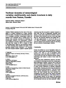
where Ui is the daily observation (PM2.5 ), γ is the model parameter, n is the number of the predictors, pij are predictors, and i is a stochastically generated random number that follows a Gaussian distribution. The statistical downscaling techniques will be applied on SDSM software that combines regression-based analyses and stochastic weather generator. The historical data will be evenly divided into two sections for model calibration and validation. SDSM first examines the correlation of PM2.5 with the most influenced predictors in model calibration. SDSM then synthesizes 20 ensembles of daily data in model validation. The model represents the most likely regression relationship between predictand-predictor [13]. Choosing predictors is a crucial process in statistical downscaling [13]. Selected predictors should satisfy the context of physical or chemical processes and also be statistically significant. In this study, we not only consider daily-correspondence predictors, but also examine predictors with lag of 1 to see effects of yesterday’s weather on PM2.5 . We use a combination of the correlation matrix, partial correlation, p-value, and knowledge from the literature to choose the influenced predictors. Firstly, correlation matrixes between the predictand and 28 predictors, as well as predictand with predictors’ lag of 1 values are calculated. Predictors that have correlation coefficient with the predictand greater than 0.25 are selected as the inputs for the SDSM model. Secondly, the partial correlation coefficient, p-value, and correlation between individual predictors are obtained by regressing predictors and predictands. Predictors that p-value is greater than 0.05 are eliminated; predictors that are highly correlated (correlation coefficient is greater than 0.7 [14]) are removed to avoid multi co-linearity; predictors that are not consistent with physical and chemical processes of PM2.5 are removed. Thirdly, the remaining predictors are regressed again with predictand on SDSM, and then 20 ensembles of PM2.5 daily data are synthesized by SDSM model. Monthly mean, monthly variance, and monthly sum are calculated for historical PM2.5 and synthesized PM2.5 to test model performance. 3.2 Artificial neural network The ANN is a perceptron model that can learn any complex non-linear relationship between a given set of predictors (meteorological variables) and the predictant (PM2.5) [9]. The general architecture of the ANN model is called multilayer perceptron, shown in Figure 1. It consists of an input layer, an output layer, and multiple hidden layers. Algorithm in every hidden layer and in output layer is WIT Transactions on Ecology and The Environment, Vol 207, © 2016 WIT Press www.witpress.com, ISSN 1743-3541 (on-line)

220 Air Pollution XXIV similar. Inputs at each layer are multiplied by their corresponding weight matrix, and summed with a bias. The summed results are the input of a nonlinear active function. The results of active function are the output of current layer as well as the inputs of the next layer, and results of output layer will be the desired data simulated by ANN model [17]. The processes of building model include training, validating, and testing processes. In this study, the Levenberg–Marquardt algorithm is employed for training and the Bayesian Regularization method is used to avoid overtraining [15–17]. During the training process, weights (wji , wkj ) and biases (bj , bk ) are updated at each iteration to minimize the error between target (observation) and output. Each iteration contains two steps: a forward operation to produce weights, bias, and a desired output, and a backward propagation of computing error to update the values of weights and bias [18]. Iterations are repeatedly processed until the error cannot be minimized anymore. The model will be implemented using the neural networks toolbox in MATLAB. We have built two ANN models to examine NCEP predictors performance (Figure 1). Model 1 evaluates all 28 NCEP predictors and their values of lag of 1, which reveals the total ability of NCEP predictors to explain PM2.5 . Model 2 evaluates only the six predictors selected in the SDSM model. Having used the same combination of predictors, the SDSM model and ANN model 2 provide a comparison of multiple linear regression and non-linear regression in the correlation of meteorological predictors and PM2.5 . The performance difference of the first and the second ANN model provides information about how much correlation the six influenced predictors can explain compared with the total correlation in the first ANN model.

4 Results and discussion 4.1 Diurnal and seasonal variation of PM2.5 Figure 2 exhibits diurnal variation of PM2.5 concentration for time period of 2003– 2014 in Toronto and Sarnia. Daily average (blue) and daily maximum (yellow) are separately calculated on weekdays and on weekends. In Toronto, there is a distinct pattern between PM2.5 concentration on weekdays and on weekends. On weekdays, the daily average of PM2.5 starts to increase at 7am and reaches its peak between 9–10am, during the morning rush hour. It drops in the following hours and starts to increase again from 7pm during the evening rush hour. On the other hand, daily average of PM2.5 on weekends is lower in general than on weekdays, and there is not a peak in the morning. Although the hourly variation of PM2.5 is relatively small on weekends, there is still a peak between 22–23pm on weekends that may due to residential heating. These results are consistent with our understanding of PM2.5 concentration in metropolitan cities, where pollutant sources are mainly from domestic emissions such as exhaust from vehicles and residential heating [19], so traffic hours and residential activities hours correspond to the time period of high emission of PM2.5 concentration. WIT Transactions on Ecology and The Environment, Vol 207, © 2016 WIT Press www.witpress.com, ISSN 1743-3541 (on-line)

Air Pollution XXIV

221

(a) The architecture of ANN model 1. Input values are observations of ln(PM2.5 ) and 56 predictors.

(b) The architecture of ANN model 2. Input values are observation of ln(PM2.5 ) and 6 predictors used in SDSM model.

Figure 1: The schematic representation of neural networks.

In Sarnia, there is no apparent difference for daily average between weekdays and weekends, because the pollutant sources are mainly industrial emissions, and 90% of major industries operate 24 hours per day 7 days per week, explaining why weekday and weekend daily averages have no obvious difference. The peak values in Sarnia appear during the periods between 8–9am and 21–22pm, which is similar to Toronto. The similar peak pattern for daily averages in Sarnia gives us a suggestion that similar meteorological conditions (predictors) have acted on PM2.5 in Toronto and in Sarnia, and the influence is similar even though the composition of PM2.5 is different due to different pollutant sources. The variance of daily maximum is much greater than daily average in Sarnia and shows no explicit pattern. This suggests that the maximum indices may largely depend on WIT Transactions on Ecology and The Environment, Vol 207, © 2016 WIT Press www.witpress.com, ISSN 1743-3541 (on-line)

222 Air Pollution XXIV

Figure 2: Diurnal variation of daily average (blue) and daily maximum (yellow) PM2.5 concentrations in weekdays and weekend in Toronto (up) and in Sarnia (down) for 2003–2014.

the summation of industrial emission rates in each industry, therefore it is difficult to detect a diurnal pattern. Figure 3 shows seasonal variation of daily average PM2.5 concentrations for 2003–2014 period. Seasonal daily averages of PM2.5 concentrations in Toronto and Sarnia all show a decrease pattern from 2003 to 2014, which exhibits a great consequence of air quality control. In both cases, we see PM2.5 concentrations is much higher in summer than in other seasons. In Toronto and Sarnia, PM2.5 concentration is 45% and 29% higher in summer than in winter respectively, and this pattern is also observed by other groups [3]. This distinct pattern brings the attention to possible particular correlation of PM2.5 concentration and meteorological variables in summer. Further conclusions will be discussed in section 4.2. 4.2 Identified meteorological variables on PM2.5 Table 3 shows the identified predictors selected in SDSM and their partial correlation and p-values. The partial correlation (partial R) shows how much the predictor can explain PM2.5 concentration under the present of other predictors, and the p-value renders the results statistically significant. Consistent with the WIT Transactions on Ecology and The Environment, Vol 207, © 2016 WIT Press www.witpress.com, ISSN 1743-3541 (on-line)

Air Pollution XXIV

223

Figure 3: Seasonal variation of daily average PM2.5 concentrations in Toronto (up) and in Sarnia (down) for 2003–2014.

assumption in 4.1, the same combination of meteorological predictors are chosen for Toronto and Sarnia models. PM2.5 concentration is influenced most by the surface zonal velocity, which can be interpreted as velocity component along a line of latitude (i.e. east-west). Among six predictors, three of them are surface velocity components, and this indicates PM2.5 concentration is a regional phenomenon. In the summer, air flow velocity at 500 hPa replaces surface air flow velocity and plays a role, so long range transport is an observably phenomenon in summer. 850 hPa geopotential height will vary depending on the temperature of the atmospheric column. Lower heights represent cyclones while higher heights represent anticyclones [20]. High pressure systems can trap pollutants and cause high PM2.5 concentrations. Low pressure systems can dramatically reduce PM2.5 concentrations through precipitation and clear the atmosphere. Both daily average and daily maximum show a strong correlation with specific humidity from the previous day. PM2.5 autoregression term shows today’s air quality is highly correlated with yesterday’s air quality. In summary, SDSM models explain 42%– 64% variation of PM2.5 concentration, and models for daily average perform better than that of daily maximum. Further analysis are applied using ANN models (Table 4). ANN model 1 studies the influence of all 56 predictors (28 NCEP + 28 NCEP of lag 1) on PM2.5 , and ANN model 2 examines the six predictors selected in SDSM model. ANN WIT Transactions on Ecology and The Environment, Vol 207, © 2016 WIT Press www.witpress.com, ISSN 1743-3541 (on-line)

224 Air Pollution XXIV model 1 shows all NCEP predictors that have strong correlation with PM2.5 from 0.79–0.85 and can explain 39%–52% variance in testing. ANN model 2 represents more than 80% information of Model 1, which shows that SDSM does select the most important predictors. SDSM model and ANN model 2 perform similarly in daily average, but ANN model 2 is better in daily maximum. Daily average more likely tends to be linear relationship with meteorological conditions, while daily maximum is more complex and tends to be a non-linear relationship.

Table 3: Statistical summary of identified predictors selected in SDSM.

Table 4: Statistical summary of models.

5 Conclusion Diurnal variations of daily average and daily maximum for PM2.5 concentration on weekdays and on weekends have been observed both in Toronto and Sarnia. The SDSM model selects six most important predictors among 28 NCEP predictors and their lag of 1, and explains 41%–64% variation of PM2.5 concentrations. ANN model 1 and model 2 show that all NCEP predictors can explain 62%– 72% variation while six selected predictors explain 52%–59% respectively. WIT Transactions on Ecology and The Environment, Vol 207, © 2016 WIT Press www.witpress.com, ISSN 1743-3541 (on-line)

Air Pollution XXIV

225

We conclude that the SDSM model has chosen the influenced predictors that represent most of the correlation between meteorological conditions and PM2.5 concentration. The selected six predictors reveal that PM2.5 concentration is a regional phenomenon in Toronto and in Sarnia, but long-range transport of PM2.5 concentration in summer is a significant phenomenon in both cases.

Acknowledgements The authors acknowledge Assist. Prof. Jane Liu and Prof. Danny Harvey from the Geography and Planning Department, University of Toronto for their professional advice. The authors appreciate the kind support from the Ministry of Environment, Ontario for providing data.

References [1] Zhang, Yaxin, et al. Photoinduced active terahertz metamaterials with nanostructured vanadium dioxide film deposited by sol-gel method. Optics express 22.9, 11070–11078, 2014. [2] World Health Organization and others. Health Effects of Particulate Matter: Policy Implications for Countries in Eastern Europe, Caucasus and Central Asia. World Health Organization Regional Office for Europe, 2013. [3] Liu, Jane, and Siliang Cui. Meteorological Influences on Seasonal Variation of Fine Particulate Matter in Cities over Southern Ontario, Canada. Advances in Meteorology 2014. [4] Tian, Jie, and Dongmei Chen. A semi-empirical model for predicting hourly ground-level fine particulate matter (PM 2.5) concentration in southern Ontario from satellite remote sensing and ground-based meteorological measurements. Remote Sensing of Environment 114.2, 221–229, 2010. [5] Tai, Amos PK, Loretta J. Mickley, and Daniel J. Jacob. Correlations between fine particulate matter (PM 2.5) and meteorological variables in the United States: Implications for the sensitivity of PM 2.5 to climate change. Atmospheric Environment 44.32, 3976–3984, 2010. [6] Jacob, Daniel J., and Darrell A. Winner. Effect of climate change on air quality. Atmospheric environment 43.1, 51–63, 2009. [7] Lambert, Steven J., and John C. Fyfe. Changes in winter cyclone frequencies and strengths simulated in enhanced greenhouse warming experiments: results from the models participating in the IPCC diagnostic exercise. Climate Dynamics 26.7-8, 713–728, 2006. [8] Wilby, R. L., and C. W. Dawson. Statistical downscaling model (SDSM) version 3.1: user manual, 2004. [9] Nunnari, Giuseppe, et al. Modelling SO2 concentration at a point with statistical approaches. Environmental Modelling & Software, 887–905, 2004. [10] Sofowote, U., Su, Y., Bitzos, M.M., and Munoz, A. Improving the Correlations of Ambient TEOM PM2.5 Data and SHARP 5030 FEM in WIT Transactions on Ecology and The Environment, Vol 207, © 2016 WIT Press www.witpress.com, ISSN 1743-3541 (on-line)

226 Air Pollution XXIV

[11] [12]

[13]

[14]

[15]

[16] [17] [18]

[19] [20]

Ontario: a Multiple Linear Regression Analysis. Journal of the Air & Waste Management Association , 64:1, 104–114, 2014. Dye, Timothy S. Guidelines for developing an air quality (Ozone and PM2. 5) forecasting program. U.S. Environmental Protection Agency, 2003. The 2011 Community Profile in the Statistics Canada’s 2011. Statistics Canada http://www12.statcan.gc.ca/ census-recensement/index-eng.cfm Wilby, R.L., Dawson, C.W.. SDSM 4.2 – A decision support tool for the assessment of regional climate change impacts. Environment Agency of England and Wales, United Kingdom, 2007. Mahmood, R., Babel, M. S. Evaluation of SDSM developed by annual and monthly sub-models for downscaling temperature and precipitation in the Jhelum basin, Pakistan and India. Theoretical and Applied Climatology 113(1-2), 27–44, 2013. Burden, Frank, and Dave Winkler. Bayesian regularization of neural networks. Artificial Neural Networks: Methods and Applications, 23–42, 2009. Demuth, Howard, and Mark Beale. Neural network toolbox for use with MATLAB, The MathWorks, Inc., 2002. Heikki N. Koivo. Neural Networks: Basics using MATLAB, The MathWorks, Inc., 2008. Okut, Hayrettin, et al. Predicting expected progeny difference for marbling score in Angus cattle using artificial neural networks and Bayesian regression models. Genetics Selection Evolution 45, 34, 2013. Air Quality in Ontario 2013 Report, Ministry of the environment and climate change, Ontario. Gramling, Robert B., et al. Taking Chances: The Coast after Hurricane Sandy. Rutgers University Press, 2016.

WIT Transactions on Ecology and The Environment, Vol 207, © 2016 WIT Press www.witpress.com, ISSN 1743-3541 (on-line)