Correntropy: Properties and Applications in Non-Gaussian ... - CiteSeerX

1

Correntropy: Properties and Applications in Non-Gaussian Signal Processing Weifeng Liu, Member, IEEE, P. P. Pokharel, Member, IEEE, and J. C. Principe, Fellow, IEEE

Abstract—The optimality of second order statistics depends heavily on the assumption of Gaussianity. In this paper, we elucidate further the probabilistic and geometric meaning of the recently defined correntropy function as a localized similarity measure. A close relationship between correntropy and M-estimation is established. Connections and differences between correntropy and kernel methods are presented. As such correntropy has vastly different properties compared with second order statistics that can be very useful in non-Gaussian signal processing, especially in the impulsive noise environment. Examples are presented to illustrate the technique. Index Terms—Generalized correlation function, information theoretic learning, kernel methods, metric, temporal principal component analysis.

I. INTRODUCTION Second order statistics in the form of correlation and in particular the mean square error (MSE) are probably the most widely utilized methodologies for quantifying how similar two random variables are. Successful engineering solutions from these methodologies rely heavily on the Gaussianity and linearity assumptions. Recently, our group has extended the concept of mean square error adaptation to include information theoretic criteria [1], which has been named Information Theoretic Learning (ITL). ITL preserves the nonparametric nature of correlation learning and MSE adaptation, i.e. the cost function is still directly estimated from data via a Parzen kernel estimator [2], but it extracts more information from the data for adaptation, and yields therefore solutions that are more accurate than MSE in non-Gaussian and non-linear signal processing [3]-[8].

Manuscript received April 6, 2006. This work was supported in part by NSF grant ECS-0300340 and ECS-0601271. The authors are with the Department of Electrical and Computer Engineering, University of Florida, Gainesville, FL 32611 USA, phone: 352-392-2682, fax: 352-392-0044 (e-mail: [email protected], [email protected], [email protected] ).

2

Inspired by ITL, we recently extended the fundamental definition of correlation function for random processes with a generalized correlation function called correntropy [9], which contains higher order moments of the PDF, but it is much simpler to estimate directly from samples than conventional moment expansions. The original definition only applies to a single random process, and it is more precisely called auto-correntropy. In this paper we extend the definition to the general case of two arbitrary random variables and provide for the first time its probabilistic and geometric meaning. This theoretical framework will help understand and apply correntropy judiciously to nonlinear, non-Gaussian signal processing. We show that correntropy is directly related to the probability of how similar two random variables are in a neighborhood of the joint space controlled by the kernel bandwidth, i.e. the kernel bandwidth acts as a zoom lens, controlling the ‘observation window’ in which similarity is assessed. This adjustable window provides an effective mechanism to eliminate the detrimental effect of outliers, and it is intrinsically different from the use of a threshold in conventional techniques. Statistics estimated from data samples usually have a geometric meaning. For instance, MSE gives the 2-norm distance in sample space. We show that correntropy induces a new metric which is equivalent to the 2-norm distance if points are close, behaves similarly to the 1-norm distance as points get further apart and eventually approaches the zero-norm as they are far apart. This geometric interpretation elucidates the robustness of correntropy for outlier rejection. The organization of the paper is as follows. After a very brief review of ITL and kernel methods to introduce the terminology, the definition and properties of correntropy are presented in section III. In section IV, the difference between MSE and correntropy is presented and the advantage of correntropy is theoretically explained based on its connection to robust M-estimation. Then in section V, some examples are presented to corroborate our understanding and to inspire readers on how to apply correntropy to their research fields. Finally, section VI summarizes the main conclusions and future lines of research.

3

II. BRIEF BACKGROUND ON ITL AND KERNEL METHODS ITL is a framework to non-parametrically adapt systems based on entropy and divergence. Renyi’s quadratic entropy of a random variable X with PDF f X ( x) is defined by H 2 ( X ) = − log ∫ f X2 ( x)dx

(1)

The Parzen estimate of the PDF, given a set of i.i.d. data {xi }iN=1 drawn from the distribution, is 1 fˆX ;σ ( x) = N

∑

N i =1

κσ ( x − xi )

(2)

where κσ ( x − xi ) is the Gaussian kernel κσ ( x − xi ) =

1 2πσ

exp(−

( x − xi ) 2 ) 2σ 2

(3)

N is the number of the data points and σ the kernel size. For simplicity, we will drop the subscript and denote it as κ (⋅) when the meaning is clear from the context. The Gaussian kernel will be the only one considered in this paper (for other Parzen kernels, most of the discussions still hold with minor modifications). The kernel size or bandwidth is a free parameter that must be chosen by the user using concepts of density estimation, such as Silverman’s rule [24], maximum likelihood or cross validation. We have experimentally verified that the kernel size affects much less the performance of ITL algorithms than density estimation [25], but a thorough treatment of this issue is beyond the scope of this paper. From the viewpoint of kernel methods, the kernel function (3) satisfies Mercer’s Theorem [11], so that it induces a nonlinear mapping Φ which transforms data from the input space to an infinite dimensional reproducing kernel Hilbert space (RKHS) F where the following equation holds κσ ( x − xi ) =< Φ ( x), Φ ( xi ) > F

(4)

< ⋅, ⋅ > F denotes inner product in F.

A nonparametric estimate of quadratic entropy directly from samples is obtained as [3] Hˆ 2 ( X ) = − log IP( X )

IP( X ) =

1 N2

N

N

∑∑ κ j =1 i =1

2σ

( x j − xi )

(5) (6)

4

IP(X) stands for information potential (IP). The PDF estimated with Parzen kernels can be thought to define an information potential field over the space of the samples [12]. It is therefore interesting to define similarity measures in this space that are not hindered by the conventional moment expansions. Towards this goal we recently proposed a similarity measure called correntropy [9] defined for random processes. Let { X (t ), t ∈ T } be a stochastic process with T being an index set. The nonlinear mapping Φ induced by the Gaussian kernel maps the data into the feature space F, where the auto-correntropy function VX (t , s ) is defined from T × T into R + given by VX (t , s ) = E[< Φ ( X (t )), Φ ( X ( s )) > F ] = E[κσ ( X (t ) − X ( s))]

(7)

We call (7) the auto-correntropy function due to the analogy with the autocorrelation of random processes and the property that its average over the lags is the IP, i.e. the argument of Renyi’s entropy [9]. We have shown that auto-correntropy is a symmetric, positive-definite function and therefore defines a new RKHS [10]. Based on auto-correntropy it is possible to derive the analytical solution of the optimal linear combiner in this space [13].

III. DEFINITION AND PROPERTIES OF CROSS CORRENTROPY A. Definition A more general form of correntropy between two arbitrary scalar random variables is defined as follows: Definition: Cross correntropy is a generalized similarity measure between two arbitrary scalar random variables X and Y defined by Vσ ( X , Y ) = E[κσ ( X − Y )]

(8)

In this paper it will be simply called correntropy. The extension of (8) to arbitrary dimensions will be addressed in a future work. In practice, the joint PDF is unknown and only a finite number of data {( xi , yi )}iN=1 are available, leading to the sample estimator of correntropy

5

1 VˆN ,σ ( X , Y ) = N

∑

N i =1

κσ ( xi − yi )

(9)

B. Properties Some important properties of correntropy are presented below. The first three are extensions of the properties presented in [9] and will therefore not be proved here. Property 1: Correntropy is symmetric: V ( X , Y ) = V (Y , X ) . Property 2: Correntropy is positive and bounded: 0 < V ( X , Y ) ≤ 1/ 2πσ . It reaches its maximum if and only if X = Y . Property 3: Correntropy involves all the even moments of the random variable E = Y − X : Vσ ( X , Y ) =

1

(−1) n ( X − Y ) 2 n ]. E[ n n! σ 2n n=0 ∞

∑2 2πσ

As σ increases, the high-order moments decay faster, so the second order moment tends to dominate and correntropy approaches correlation. This has been verified in practice for kernel sizes 20 times larger than the value given by Silverman’s rule for the data. Due to the expected value operator, the issue of kernel size selection in correntropy is different from density estimation. As will be practically demonstrated, the performance sensitivity of correntropy to the kernel size is much less than what could be expected from density estimation. Property 4: Assume i.i.d. data {( xi , yi )}iN=1 are drawn from the joint PDF f X ,Y ( x, y ) , and fˆX ,Y ;σ ( x, y ) its Parzen estimate with kernel size σ . The correntropy estimate with kernel size σ ' = 2σ is the integral of fˆX ,Y ;σ ( x, y ) along the line x = y [19] +∞

Vˆ

( X ,Y ) = 2σ

∫

fˆX ,Y ;σ ( x, y ) |x = y = u du

(10)

−∞

Proof: Using the two dimensional radially symmetric Gaussian kernel to estimate the joint PDF, we have 1 fˆX ,Y ;σ ( x, y ) = N

where

N

⎛ x ⎞ ⎛ xi ⎞

∑ Kσ (⎜ y ⎟ − ⎜ y ⎟) i =1

⎝ ⎠ ⎝

i

⎠

(11)

6

T

⎛σ 2

with Σ = ⎜

⎝ 0

⎛ x⎞ ⎛ x⎞ 1 1⎛ x⎞ exp(− ⎜ ⎟ Σ −1 ⎜ ⎟) Kσ (⎜ ⎟) = 1/ 2 2⎝ y⎠ ⎝ y ⎠ 2π | ∑ | ⎝ y⎠

(12)

⎛ x⎞ Kσ (⎜ ⎟) = κσ ( x) ⋅ κσ ( y ) ⎝ y⎠

(13)

0 ⎞ ⎟. σ2⎠

It is easy to see that

So 1 fˆX ,Y ;σ ( x, y ) = N

∑

N i =1

κσ ( x − xi ) ⋅ κσ ( y − yi )

(14)

Integrating (14) along the line x = y , we obtain +∞

∫

fˆX ,Y ;σ ( x, y ) |x = y = u du

−∞ +∞

=

1 ∫−∞ N

1 = N =

1 N

N

∑ κσ ( x − x ) ⋅ κσ ( y − y ) | i

i =1

i

x = y =u

du (15)

N +∞

∑ ∫ κσ (u − x ) ⋅ κσ (u − y )du i

i =1 −∞ N

∑κ i =1

2σ

( xi − yi ) = Vˆ

i

2σ

( X , Y ).

This completes the proof. According to the conditions of the Parzen method [2], when σ goes to zero and the product Nσ to infinity, fˆX ,Y ;σ ( x, y ) approaches the true PDF f X ,Y ( x, y ) , therefore we also have lim V ( X , Y ) = lim ∫∫ κσ ( x − y ) f XY ( x, y )dxdy

σ →0

σ →0

x, y

= ∫∫ δ ( x − y ) f X ,Y ( x, y )dxdy = x, y

(16)

+∞

∫

f X ,Y ( x, x)dx

x =−∞

In practical applications, the estimation of correntropy is done only with a finite number of samples, which sets a lower bound on the kernel size, since too small a kernel size will lead to meaningless estimation [2]. When the kernel size used in correntropy is σ , its rectangle approximation has a bandwidth π / 2σ and let us assume that the joint PDF is smooth in this bandwidth. Then a more precise evaluation of

7

correntropy is Vσ ( X , Y ) ≈ P (| Y − X |< π / 2σ )

2πσ

(17)

Property 5: Assume the samples {( xi , yi )}iN=1 are drawn from the joint PDF f X ,Y ( x, y ) . Define the error random variable E = Y − X , and fˆE ;σ (e) as the Parzen estimate of the error PDF from data {(ei = xi − yi )}iN=1 . Then Vˆσ ( X , Y ) is the value of fˆE ;σ (e) evaluated at the point e = 0 , i.e., Vˆσ ( X , Y ) = fˆE ;σ (0).

(18)

1 N Vˆσ ( X , Y ) = ∑ i =1 κσ ( xi − yi ) N 1 N = ∑ i =1 κσ (ei ) = fˆE ;σ (0). N

(19)

Proof: By (9)

which completes the proof. It is important to study the statistical properties of the correntropy estimator. First note that Vσ ( X , Y ) = Ε[κσ ( X − Y )] = E[κσ ( E )]

(20)

= ∫ κσ (e) f E (e)de e

It is also obvious that +∞

f E (0) = p ( X = Y ) =

∫

f X ,Y ( x, x)dx

(21)

x =−∞

Now, the study of the mean and variance of VˆN ;σ ( X , Y ) is quite straightforward in the context of Parzen estimation [2]. Indeed, E[VˆN ,σ ( X , Y )] = Vσ ( X , Y ) lim

N →∞ ,σ → 0

(22)

E[VˆN ,σ ( X , Y )] = f E (0)

var[VˆN ,σ ( X , Y )] = N −1 var[κσ ( E )] lim

N →∞ ,σ → 0

∞

Nσ var[VˆN ,σ ( X , Y )] = f E (0) ∫ (κ1 ( z )) 2 dz −∞

(23) (24) (25)

where κ1 ( z ) is the Gaussian kernel with σ = 1 . Among these properties, (25) is the most important and its proof can be essentially found in [2]. Therefore,

8

under the condition of N → ∞ , VˆN ,σ ( X , Y ) is an unbiased estimator of Vσ ( X , Y ) and consistent in mean square. Further, under the conditions Nσ → ∞ and σ → 0 , VˆN ,σ ( X , Y ) is an asymptotically unbiased estimator of f E (0) and consistent in mean square. Let us assume the error PDF is Gaussian, i.e. 1

f E (e ) =

2πσ E

exp( −

e2 2σ E 2

)

(26)

Then we have Vσ = 1

2π (σ 2 + σ E 2 )

(27)

2πσ E

(28)

V0 =: lim Vσ = 1 σ →0

A simple calculation shows | (Vσ − V0 ) / V0 |< 0.05 if σ < 0.32σ E . In the case of σ 2 F

(34)

Proof: Using the notation in property 6, V ( X , Y ) = E[∑ i =1ϕi ( X )ϕi (Y )] M

= ∑ i =1 E[ϕi ( X )]E[ϕi (Y )] =< E[Φ ( X )], E[Φ (Y )] >F M

(35)

by the independence assumption. This completes the proof. This property can be called uncorrelatedness in feature space and is a new, easily computable measure of independence between X and Y. Additionally, this property can be interpreted in terms of PDF. If X and Y are independent, f X ,Y ( x , y ) = f X ( x ) f Y ( y )

(36)

Using Parzen window to estimate these PDFs, 1 fˆX ,Y ;σ ( x, y ) = N

N

∑ κσ ( x − x ) ⋅ κ σ ( y − y ) i

i =1

i

(37)

N

1 fˆX ;σ ( x) = N

∑ κσ ( x − x )

1 fˆY ;σ ( y ) = N

∑ κσ ( y − y )

(38)

i

i =1 N

(39)

i

i =1

Integrating (36) along the line x=y and using (37), (38), (39) yields 1 N

N

∑κ i =1

2σ

( xi − yi ) ≈

1 N2

N

N

j

i

∑∑ κ

2σ

( x j − yi )

(40)

which is a sample estimate approximation of (34). The approximation in (40) is due to the Parzen estimates.

10

When σ tends to zero and the product Nσ to infinity, strict equality holds. Using the analogy of potential fields, the term on the right hand side of (40) is called the Cross Information Potential (CIP). When X = Y , it reduces to IP. From the viewpoint of kernel methods, f X (⋅) = E[Φ ( X )] , fY (⋅) = E[Φ (Y )] are two points in the RKHS, and CIP is exactly the inner product between the vectors created by these two PDFs. Equation (40) bears resemblance to the constrained covariance proposed by Gretton et al in [23], which is a strong measure of independence according to the work of Jacod and Protter on independence characterization through covariance operator in function spaces [23]. These authors constrained the covariance operator in a closed ball of a reproducing kernel Hilbert space and converted the measure into a matrix norm of Gram matrices. However, our measure starts directly from Parzen estimates of PDFs and is a much simpler, while possibly weaker, measure of independence. Further analysis and applications of this property in independent component analysis (ICA) will be pursued in future work. Property 8: Correntropy, as a sample estimator, induces a metric in the sample space. Given two vectors X = ( x1 , x2 ,..., xN )T and Y = ( y1 , y2 ,..., y N )T in the sample space, the function CIM( X , Y ) = (κ (0) − V ( X , Y ))1/ 2

defines a metric in the sample space and is named as the Correntropy Induced Metric (CIM). Proof: This property highlights the geometric meaning of correntropy in the sample space. To be a metric CIM must be: 1) Non-negativity. CIM( X , Y ) ≥ 0 by Property 2. 2) Identity of indiscernibles. CIM( X , Y ) = 0 if and only if X = Y by Property 2. 3) Symmetric by Property 1. 4) Triangle inequality: CIM( X , Z ) ≤ CIM( X , Y ) + CIM(Y , Z ) . The proof is based on the kernel mapping and a vector construction in a feature space which is a well defined Hilbert space. For X and Y, we construct two new vectors X% = [Φ ( x1 ); Φ ( x2 );...; Φ ( xN )] and Y% = [Φ ( y1 ); Φ ( y2 );...; Φ ( yN )] in the Hilbert space FN . The Euclidean distance ED( X% , Y% ) is

11

ED( X% ,Y% ) = (< ( X% − Y% ), ( X% − Y% ) >)1/ 2 = (< X% , X% > −2 < X% , Y% > + < Y% , Y% >)1/ 2 N

N

i =1

i =1

N

= (∑ κ ( xi − xi ) − 2∑ κ ( xi − yi ) + ∑ κ ( yi − yi ))1/ 2

(41)

i =1

= [2 N ⋅ (κ (0) − V ( X , Y ))]

1/ 2

= 2 N ⋅ CIM( X , Y )

Therefore CIM( X , Z ) = ED( X% , Z% ) / 2 N ≤ ED( X% , Y% ) / 2 N + ED( Z% , Y% ) / 2 N

(42)

= CIM( X , Y ) + CIM(Y , Z )

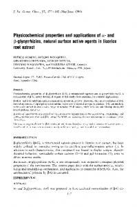
This completes the proof. It can also be shown that this metric is translation invariant for translation invariant kernels like the Gaussian kernel, so we can denote V ( X , Y ) as V (Y − X ) . However, CIM is not homogenous so it can not further induce a norm on the sample space. Fig. 1 shows the contours of the distance from X to the origin in a 2 dimensional space. The interesting observation is as follows: when two points are close, CIM behaves like an L2 norm (which is clear from the Taylor expansion of property 3) and we call this area the Euclidean zone; outside of the Euclidean zone CIM behaves like an L1 norm which is named the Transition zone; eventually in the Rectification zone as two points are further apart, the metric saturates and becomes insensitive to distance (approaching a L0 norm). This property inspired us to investigate the inherent robustness of CIM. Another important observation is that the kernel bandwidth σ controls the scale of the CIM norm. A small kernel size leads to a tight linear (Euclidean) region and to a large L0 region, while a larger kernel size will enlarge the linear region. Note also that for points far away from the origin, the metric becomes radially anisotropic, i.e. the distance becomes dependent on the direction. It is remarkable that a single parameter has such a tremendous impact on the evaluation of radial distances from any given point unlike what happens in the more traditional Lp norms. While bringing flexibility, there is still a need to choose appropriately the kernel size in practical applications.

12

2 0. 45

0. 5

0.4

5 0.5

5 0.

45 0.

1.5

0.5 5

0. 35 4 0.

1

0.3

5 0.4

0.5

3 0.

0.2 5

25 .2 0. 0

0.15

0.4

0 25 0.

-0.5

0. 2

0.05 0.15

5 0.2

0. 4 5

-1

4 0. 35 0.

0.3

0. 4

5 0.5

45 0.

5 0.

0. 45

0.4

-1.5

-1

5 0.4 0.5

0.35

-1.5 0.5 5 -2 -2

0.4 5

0. 3

0. 3

5 0.3

0. 1

0. 4

0.2

0.1

0.4

x2

35 0.

35 0.

-0.5

0

0.5

1

1.5

2

x1

Fig. 1. Contours of CIM(X,0) in 2D sample space (kernel size is set to 1).

Property 9: Let {xi }iN=1 be a data set. The correntropy kernel induces a scalar nonlinear mapping η which maps the signal as {η x (i)}iN=1 while preserving the similarity measure in the sense E[η x (i ) ⋅η x (i + t )] = V (i, i + t ) = E[κ ( x(i ) − x(i + t ))], 0 ≤ t ≤ N − 1

(43)

And the square of the mean of the transformed data is an asymptotic estimate of the information potential of the original data as N → ∞ . Proof: The existence of this nonlinear mapping η is proved in [13] using results from [10]. Here we prove the second part of the property. Denote mη as the mean of the transformed data mη =

Therefore

1 N

N

∑η i =1

x

(i )

(44)

13

mη 2 =

1 N2

N

N

∑∑η i =1 j =1

x

(i )η x ( j )

(45)

Rewriting (43) in the sample estimate form, asymptotically we have N −t

∑η i =1

N −t

x

(i ) ⋅η x (i + t ) = ∑ κ ( x(i) − x(i + t ))

(46)

i =1

with fixed t and as N → ∞ . We arrange the double summation (45) as an array and sum along the diagonal direction which yield exactly the autocorrelation function of the transformed data at different lags, thus the correntropy function of the input data at different lags, i.e. 1 N2

N

N

∑∑η i =1 j =1

x

(i )η x ( j ) =

N −1 N 1 N −1 N − t η (i)η x (i + t ) + ∑ ∑ η x (i)η x (i − t )) ( 2 ∑∑ x N t = 0 i =1 t =1 i =1+ t

N −1 N 1 N −1 N −t ≈ 2 (∑∑ κ ( x(i ) − x(i + t )) + ∑ ∑ κ ( x(i) − x(i − t ))) N t = 0 i =1 t =1 i =1+ t 1 N N = 2 ∑∑ κ ( x(i ) − x( j )) N i =1 j =1

(47)

As observed in (47), when the summation indices are far from the main diagonal, smaller and smaller data sizes are involved which leads to poorer approximations. Notice that this is exactly the same problem when the auto-correlation function is estimated from windowed data. As N approaches infinity, the estimation error goes to zero asymptotically. In other words, the mean of the transformed data induced by the correntropy kernel asymptotically estimates the square root of the information potential and thus the entropy of the original data. This property corroborates further the name of correntropy given to this similarity measure. Property 10: The auto-correntropy function defined by (7) is a reproducing kernel. This property is proved in [9] and will be only interpreted here. Correntropy can be interpreted in two vastly different feature spaces. One is the RKHS induced by the Gaussian kernel, which is widely used in kernel machine learning. The elements on this RKHS are infinite dimensional vectors expressed by the eigen-functions of the Gaussian kernel [11], and they lie on the first quadrant of a sphere since Φ ( x) = κ (0) = 1/ 2πσ [9]. Correntropy performs statistical inference on the projected samples in this 2

14

sphere. A full treatment of this view requires a differential geometry approach to take advantage of the manifold properties. The second feature space is the RKHS induced by the correntropy kernel itself where elements are random variables and the inner product is defined by the correlation [10]. With this interpretation, correntropy can be readily used for statistical inference, and provides a straightforward way to apply conventional optimal algorithms based on inner products in a RKHS that is nonlinearly related to the input space. Solutions of a nonlinear (w.r.t. to the input space) Wiener filter [13] and of a nonlinear minimum average correlation energy (MACE) filter [26] have already been achieved. The problem is that products of transformed samples must be approximated by the kernel evaluated at the samples to implement the computation, which is only valid in the mean (see property 9). This limits performance but the results are very promising. Later in this paper we will extend correntropy to the estimation of a nonlinear Karhunen Loeve transform. In this section, most results are new contributions. For the first time a detailed explanation of the probabilistic meanings of correntropy and an analysis of the mean-variance of the correntropy estimator are presented in properties 4 and 5. Properties 6 and 7 show interpretations of correntropy in connection to kernel methods. Property 8 is one of the main results in this paper, defining a new metric in sample space which is the mathematical foundation for regression applications in section V. The proof in property 9 is also novel and together with property 10 it will be used to derive correntropy temporal principal component analysis in the following section.

IV. COMPARISON BETWEEN MSE AND CORRENTROPY Let X and Y be two random variables and E = Y − X . MSE( X , Y ) is defined as MSE( X , Y ) = E[( X − Y ) 2 ] = ∫∫ ( x − y ) 2 f XY ( x, y ) dxdy = ∫ e 2 f E (e) de x, y

whereas

e

(48)

15

V ( X , Y ) = E[κ ( X − Y )] = ∫∫ κ ( x − y ) f XY ( x, y )dxdy = ∫ κ (e) f E (e)de.

(49)

e

x, y

Notice that the MSE is a quadratic function in the joint space with a valley along the x = y line. Since similarity quantifies how different X is from Y in probability, this intuitively explains why MSE is a similarity measure in the joint space. However, the quadratic increase for values away from the x = y line has the net effect of amplifying the contribution of samples that are far away from the mean value of the error distribution and it is why Gaussian distributed residuals provide optimality for the MSE procedure. But it is also the reason why other data distributions will make the MSE non-optimal, in particular if the error distribution has outliers, is non-symmetric, or has nonzero mean. Comparing MSE with correntropy, we conclude that these two similarity measures are assessing similarity in rather different ways: Correntropy is local whereas MSE is global. By global, we mean that all the samples in the joint space will contribute appreciably to the value of the similarity measure while the locality of correntropy means that the value is primarily dictated by the kernel function along the x = y line. Therefore, correntropy of the error (51) can be used as a new cost function for adaptive systems training, which will be called the maximum correntropy criterion (MCC). MCC has the advantage that it is a local criterion of similarity and it should be very useful for cases when the measurement noise is non-zero mean, non-Gaussian, with large outliers. It is also easier to estimate than the MEE criterion proposed in [1]. Furthermore, we can put MCC in a more general framework by showing that it bears a close relationship with M-estimation [21]. M-estimation is a generalized maximum likelihood method proposed by Huber to estimate parameters θ under the cost function min ∑ i =1 ρ (ei | θ ) , where ρ is a differentiable function N

θ

satisfying: 1) ρ (e) ≥ 0 2) ρ (0) = 0 3) ρ (e) = ρ (−e)

16

4) ρ (ei ) ≥ ρ (e j ) for | ei |>| e j | . In the case of adaptive systems, θ is a set of adjustable parameters and ei are errors produced by the system during supervised learning. This general estimation is also equivalent to a weighted least square problem as N

min ∑ w(ei )ei 2 θ

(50)

i =1

The weight function w(e) is defined by w(e) = ρ '(e) / e where ρ ' is the derivative of ρ . Defining ρ (e) = (1 − exp(−e2 / 2σ 2 )) / 2πσ it is easy to see that ρ satisfies all the conditions listed above. Moreover, it corresponds to the kernel of the error as can be easily shown as N

N

min ∑ ρ (ei ) = min ∑ (1 − exp(−ei 2 / 2σ 2 )) / 2πσ θ

θ

i =1

i =1

N

N

⇔ max ∑ exp( −ei / 2σ ) / 2πσ = max ∑ κσ (ei ) 2

θ

(51)

2

i =1

θ

i =1

The weighting function in this case is w(e) = exp( −e 2 / 2σ 2 ) / 2πσ 3

(52)

For comparison, the weighting function of Bi-square is ⎧[1 − (e / h) 2 ]2 | e |≤ h wBi (e) = ⎨ | e |> h ⎩0

(53)

where h is a tuning constant. It turns out that the square of the Taylor expansion of (52) to the first order is the weight function of Bi-square and the kernel size σ serves as the tuning constant in Bi-square. Notice that the weighting function is solely determined by the choice of ρ in the cost function and does not depend on the adaptive system. For example, the MSE cost function uses a constant weighting function. In that sense, the Gaussian like weighting function attenuates the large error terms so that outliers would have a less impact on the adaptation. It is the first time a close relationship between M-estimation and methods of ITL is established, although their superior performances in impulsive environments were repeatedly reported [7]-[9]. It is also interesting that there is no threshold in correntropy. The kernel size controls all the properties of the estimator. Moreover, this connection may provide one practical way to choose an appropriate kernel size for

17

correntropy.

V. APPLICATIONS A. Robust Regression In the first example, we consider the general model of regression Y = f ( X ) + Z where f is an unknown function, Z is a noise process and Y is the observation. A parametric approximator g ( x; w) (specified below) is used to discover this function and alleviate the effect of noise as much as possible. Let the noise probability density function be an impulsive Gaussian mixture pZ ( z ) = 0.9 × N(0, 0.1) + 0.1× N(4, 0.1) . In MSE, the optimal solution is found by min J ( w) = w

1 M

M

∑ ( g ( x ; w) − y ) i =1

i

2

i

(54)

Here {( xi , yi )}iM=1 are the training data. Under the maximum correntropy criterion (MCC), the optimal solution is found by max J ( w) = w

1 M

M

∑ κσ ( g ( x ; w) − y ) i =1

i

i

(55)

The first example uses a first degree polynomial system for simplicity, i.e. g ( x; w) = w1 x + w2 . f ( x) = ax + b with a = 1 and b = 0 . Since the ultimate performance of the MCC criterion is under

investigation, the kernel size is chosen by systematically searching for the best result using either a priori knowledge of the noise distribution, or simply scanning when the problem justifies this solution. Performance sensitivity with respect to kernel size will be quantified experimentally in Tables and will be compared with the kernel size estimated by Silverman’s rule, one of the most widely used kernel density estimation heuristics. The data length is set small on purpose, M = 100. Steepest descent is used for both criteria. Under the MSE criterion, the learning rate is set to 0.001 and the system is trained for 500 epochs (long enough to guarantee it reaches its global solution). In the MCC experiment, we first train the system with MSE criterion during the first 200 epochs (which is equivalent to kernel size annealing [1] as shown in Properties 3 and 8), and switch the criterion to MCC during the next 300 epochs. The learning rate is set to

18

0.001 and the kernel size is 0.5 which performs best on test data. We run 50 Monte Carlo simulations for the same data with 50 different starting points. The average estimated coefficients for MSE are [0.484 0.679] and [0.020 0.983] for MCC. The average learning curves are shown in Fig.2, along with its standard deviation. For comparison, we also include the result of Minimum Error Entropy (MEE) [1] with the bias set at the mean of the desired response. MEE is independent of the mean of the distribution, but with the bias set as explained it is also sensitive to the non-zero mean noise. 1.2 MCC MSE MEE

Intrinsic Error Power

1 0.8 0.6 0.4 0.2 0 0

100

200

300

400

500

epochs Fig. 2. Average learning curves with error bars of MCC, MSE and MEE. g

5 f(x) 4

Y g(x) by MSE

3

g(x) by MCC g(x) by MEE

y,f,g

2 1 0 -1 -2 -1

-0.5

0 0.5 1 x Fig. 3. Regression results with criteria of MSE, MCC, and MEE respectively. The observation Y is corrupted with positive impulsive noise; the fit from MSE (dash-dot line) is shown shifted and skewed; the fit from MCC (solid line) matches the desired (dotted) quite well; the fit from MEE is shifted but not skewed.

19

When MSE criterion is used, g ( x) is shifted by the non-zero-mean noise and slanted by the outliers due to the global property of MSE (Fig.3). Now we see the importance of correntropy with its local property. In other words, correntropy has the ability of being insensitive to the peak in the noise PDF tail, and effectively handle the bulk of residuals around the origin (Property 5). Although the main purpose of this example is to highlight the robustness of correntropy, we feel obligated to compare with the existing robust fitting methods such as Least Absolute Residuals (LAR) and Bi-square Weights (BW) [18]. The parameters of these algorithms are the recommended settings in MATLAB. Another set of 50 Monte Carlo simulations are run with different noise realizations and different starting points. All the results are summarized in Table I in terms of intrinsic error power (IEP) which is estimated as E[( g ( X ; w) − f ( X )) 2 ] on the test set. All the results in the tables are in the form of ‘average ± standard

deviation’. Notice that the intrinsic error power compares the difference between the model output and the true system (without the noise added). The performance of MCC is much better than LAR, and when regarded as a L1 norm alternative, correntropy is differentiable everywhere and to every order. Furthermore, notice that there is no threshold for MCC, just the selection of the kernel size. Moreover, the algorithm complexity of MEE is O(M2) whereas MSE, MCC, BS and LAR are all O(M). TABLE I REGRESSION RESULTS SUMMARY

MSE MCC MEE LAR BW

a

b

1.0048±0.1941 0.9998±0.0550 0.9964±0.0546 1.0032±0.0861 1.0007±0.0569

0.3969±0.1221 0.0012±0.0355 0.3966±0.1215 0.0472±0.0503 0.0010±0.0359

IEP 0.1874±0.1121 0.0025±0.0026 0.1738±0.1049 0.0072±0.0066 0.0025±0.0025

Next, the effect of the kernel size on MCC is demonstrated. We choose 7 kernel sizes: 0.1, 0.2, 0.5, 1, 2, 3, and 4. For each kernel size, 50 Monte Carlo simulations with different noise realizations are run to estimate the intrinsic error power and its standard deviation. The results are presented in Table II. MCC performs very well when the kernel size is in the range of [0.2, 2]. Intuitively, if the data size is large, a small kernel size shall be used so that MCC searches with high precision (small estimator bias) for the maximum

20

position of the error PDF. However, if the data size is small, the kernel size has to be chosen as a compromise between estimation efficiency (small estimator variance) and outlier rejection. Nevertheless, MCC using large kernel sizes will perform no worse than MSE due to correntropy unique metric structure as shown in property 8. If one sets the kernel size by applying Silverman’s rule to the error signal of each iteration [24], σ Sm = 1.06 ∗ min{σ E , R /1.34} ∗ M −1/ 5

(56)

where σ E is the error power and R is the error interquartile range, σ SM varies between [1.8, 3] during the adaptation, which is in the neighborhood of the best values as shown in Table II. TABLE II EFFECTS OF KERNEL SIZE ON MCC

σ 0.1 0.2 0.5 1.0 2.0 3.0 4.0 Silverman’s

IEP 0.0511±0.0556 0.0059±0.0050 0.0024±0.0024 0.0022±0.0022 0.0113±0.0109 0.0502±0.0326 0.0950±0.0558 0.0053±0.0052

In the fourth set of simulations, we investigate the effect of the mean and variance of the outliers. First, we keep the variance at 0.1 and set the mean of the outliers to be 0.2, 0.5, 1, and 2 respectively. The performance of MCC, BW and LAR are summarized in Table III. In short, large-mean outliers are easy to reject while small-value outliers naturally have small effect on the estimation. Next, we set the mean of the outliers to be 4 and vary the variance. The results are shown in Table IV. As we see, MCC performs very well under a variety of circumstances. The kernel size is set at 0.5 throughout this set of simulations. TABLE III EFFECTS OF THE MEAN OF THE OUTLIERS Outliers mean 0.2 0.5 1.0 2.0

IEP by MCC

IEP by BW

0.0026±0.0021 0.0045±0.0047 0.0028±0.0033 0.0024±0.0023

0.0023±0.0019 0.0048±0.0043 0.0053±0.0059 0.0026±0.0027

IEP by LAR 0.0030±0.0026 0.0054±0.0050 0.0048±0.0048 0.0060±0.0053

TABLE IV EFFECTS OF THE VARIANCE OF THE OUTLIERS

21

Outliers variance 0.2 0.5 1.0 2.0 4.0

IEP by MCC

IEP by BW

IEP by LAR

0.0031±0.0032 0.0021±0.0018 0.0025±0.0025 0.0034±0.0038 0.0022±0.0022

0.0026±0.0024 0.0022±0.0019 0.0025±0.0024 0.0032±0.0034 0.0023±0.0024

0.0072±0.0062 0.0059±0.0048 0.0055±0.0051 0.0061±0.0056 0.0069±0.0068

A second, more complex and nonlinear, regression experiment is conducted to demonstrate the efficiency of MCC. Let the noise PDF be pZ ( z ) = (1 − ε ) × N(0, 0.1) + ε × N(4, 0.1) and f ( X ) = sinc( X ) , X ∈ [−2, 2] . A multilayer perceptron (MLP) is used as the function approximator g ( x; w) with 1 input unit, 7 hidden units with tanh nonlinearity and 1 linear output. The data length is M = 200. Under the MSE criterion, the MLP is trained for 500 epochs with learning rate 0.01 and momentum rate 0.5. Under the LAR criterion, 600 epochs are used with learning rate 0.002 and momentum rate 0.5. In the MCC case, MSE criterion is used for the first 200 epochs and switched to MCC for the next 400 epochs with learning rate 0.05 and momentum rate 0.5. Different values of ε are tried to test the efficiency of MCC against LAR. 50 Monte Carlo simulations are run for each value. The results are in Table V. The kernel size in MCC is chosen as σ =1 for best results. An outstanding result is that MCC can attain the same efficiency as MSE when the noise is purely Gaussian due to its unique property of ‘mix norm’ whereas LAR can not. TABLE V NONLINEAR REGRESSION RESULTS SUMMARY

ε

IEP by MCC

IEP by MSE

IEP by LAR

0.1 0.05 0.01 0

0.0059±0.0026 0.0046±0.0021 0.0039±0.0017 0.0040±0.0019

0.2283±0.0832 0.0641±0.0325 0.0128±0.0124 0.0042±0.0020

0.0115±0.0068 0.0083±0.0041 0.0058±0.0025 0.0061±0.0028

Next we fix ε = 0.05 and choose different kernel sizes to show that a wide range of values can be used in this problem. A noteworthy observation and corollary of property 8 is that when large kernel sizes are employed, MCC reduces to MSE. In other words, MCC using large kernel sizes will never perform worse than MSE. The kernel size estimated by Silverman’s rule on the error signal is around 0.2 during adaptation. For this problem this heuristic is not the best possible value, but it is still far better that the MSE solution.

22

TABLE VI EFFECTS OF KERNEL SIZE ON MCC IN NONLINEAR REGRESSION

σ

IEP

0.2 0.5 1.5 2.0 4.0 10 Silverman’s

0.01476±0.01294 0.00594±0.00243 0.00556±0.00252 0.00854±0.00737 0.01553±0.00840 0.06020±0.02489 0.01220±0.00612

6 Desired Observation MSE MCC LAR

5

Y, f(X), g(X)

4 3 2 1 0 -1 -2

-1.5

-1

-0.5

X0

0.5

1

1.5

2

Fig. 4. Nonlinear regression results by MSE, MCC and LAR respectively.

B. Temporal Principal Component Analysis with Correntropy In this example, we present a correntropy extension to the Karhunen-Loeve transform that will be called here temporal principal component analysis (TPCA) which is widely utilized in subspace projections [16]. Suppose the signal is {x(i), i = 1, 2,..., N + L − 1} and we can map this signal as a trajectory of N points in the reconstruction space of dimension L. With the data matrix L x( N ) ⎤ ⎡ x(1) x(2) ⎥ X = ⎢⎢ M M O M ⎥ ⎢⎣ x( L) x( L + 1) L x( N + L − 1) ⎥⎦ L× N

(57)

Principal Component Analysis estimates the eigen-filters and principal components (PC) [16]. We review this technique in a different way here to extend the method easily to correntropy TPCA. The autocorrelation matrix and Gram matrix are denoted as R and K respectively, and written as

23

r (1) L r ( L − 1) ⎤ ⎡ r (0) ⎢ r (1) O O M ⎥⎥ R = XXT ≈ N × ⎢ ⎢ M O r (0) r (1) ⎥ ⎢ ⎥ − L r L r r ( 1) (1) (0) ⎦ L× L ⎣

(58)

r (1) L r ( N − 1) ⎤ ⎡ r (0) ⎢ r (1) O O M ⎥⎥ K = XT X ≈ L × ⎢ ⎢ M O r (0) r (1) ⎥ ⎢ ⎥ r (0) ⎦ N × N ⎣ r ( N − 1) L r (1)

(59)

where r (k ) = E[ x(i ) x(i + k )] is the autocorrelation function of x. When N and L are large, (58) and (59) are good approximations. In the following derivation, we will see that L is actually not involved in the new algorithm, so we can always assume L is set appropriately to the application. Assuming L < N , by Singular Value Decomposition (SVD) we have X = UDV T

(60)

where U, V are two orthonormal matrices and D is a pseudo-diagonal L × N matrix with singular values { λ1 , λ2 ,... λL } as its entries. Therefore,

R = XXT = UDDT UT

(61)

K = XT X = VDT DV T

(62)

From (61) and (62), the columns of U and V are eigenvectors of R and K respectively. Rewriting (60) as UT X = DV T

(63)

U i T X = λi Vi T , i = 1, 2,..., L

(64)

or equivalently,

Here U i and Vi are the i-th columns of U and V respectively. This equation simply shows that the projected data onto the i-th eigenvector of R is exactly the scaled i-th eigenvector of K. This derivation provides another viewpoint to understand why Kernel PCA obtains the principal components from the Gram matrix [17]. As we see, for the conventional PCA, we can either obtain the principal components by eigen-decomposing the autocorrelation matrix and then projecting the data or by eigen-decomposing the Gram matrix directly. Moreover, by property 9, there exists a scalar nonlinear mapping η (⋅) (not Φ ) which maps the signal as

24

{η x (i ), i = 1, 2,..., N + L − 1} while preserving the similarity measure

E[η x (i ) ⋅η x ( j )] = E[κ ( x(i ) − x( j ))]

(65)

In other words, the autocorrelation function of η X (i ) is given by the correntropy function of x. With these results, the correntropy extension to temporal PCA is straightforward. We simply replace the auto-correlation entries with the correntropy entries in (59) and obtain the principal components by eigen-decomposition of the new Gram matrix K. Therefore, correntropy TPCA is similar to kernel PCA in the sense that none has access to the projected data, so the only way to obtain the principal components is by eigen-decomposing the Gram matrix. However, we are talking about entirely different feature spaces as explained in property 10. As a practical example, we apply correntropy TPCA (CTPCA) to a sinusoidal signal corrupted with impulsive noise x( m) = sin(2π fm) + A ⋅ z (m)

(66)

for m = 1, 2,..., N + L − 1 . z (m) is a white noise process drawn from the PDF pZ (z) = 0.8× N(0,0.1) + 0.1× N(4,0.1) + 0.1× N(−4,0.1)

(67)

We set N = 256 , f = 0.3 and generate 3N data to estimate N point autocorrelation and correntropy functions. For TPCA, the larger the subspace (larger L), the higher the Signal Noise Ratio (SNR) is. For a fair comparison, we choose to eigen-decompose the N-by-N Gram matrix for both methods. Results by eigen-decomposing the L-by-L autocorrelation matrix and then projecting the data are also presented for comparison. For each case in Table V, 1000 Monte Carlo trials with different noise realizations are run to evaluate the improvement of CTPCA upon TPCA. For A = 5 , the probability of detecting the sinusoidal signal successfully as the largest peak in the spectrum is 100% for CTPCA, compared with 15% for N-by-N autocorrelation (Fig. 5). The kernel size is set to σ = 1 in CTPCA throughout this simulation. In this particular application of finding sinusoids in noise, the kernel size can be scanned until the best line spectrum is obtained. In CTPCA, the second principal component is used instead of the first one, because the transformed data is

25

not centered in the feature space and the mean introduces a large DC component that is picked as the first 1

Observation clean signal

Average FFT magnitude

0.5 0 0

0.1

0.2

0.3

0.4

0.5

0.1

0.2

0.3

0.4

0.5

0.2 0.1 0 0 1 0.5 0 0

0.1

0.2 0.3 0.4 0.5 Normalized frequency Fig. 5. Principal component analysis of sinusoidal signal in impulsive noise. (top) FFT of clean sinusoidal signal and noisy observation (A=5); (middle) Average of FFT of first principal component by EVD N-by-N auto-correlation matrix; (bottom) Average of FFT of second principal component by EVD N-by-N correntropy matrix.

component. This can be easily shown as follows. We denote C as the correntropy matrix, Cc as the centered correntropy matrix, mη as the mean of the transformed data, 1N as an N-by-1 column vector with all entries equal to 1 and 1N × N as an N-by-N matrix with all entries equal to 1. Thus, Cc = C − mη2 ⋅1N ⋅1TN

(68)

If we normalize the eigenvector 1N to be unit norm, the corresponding eigenvalue is Nmη2 which can be very large if N is large as in this example. Therefore, the first principal component of the correntropy matrix in this example is always a DC component. The method widely used in kernel methods to calculate the centered Gram matrix [20] also applies here. Cc = C − 1N × N ⋅ C / N − C ⋅1N × N / N + 1N × N ⋅ C ⋅ 1N × N / N 2

(69)

Simulation results in Table VII shows the centering CTPCA works very well.

A 5 4 2

CTPCA (2nd PC) 100% 100% 100%

TABLE VII RESULTS OF TIME SERIES PRINCIPAL COMPONENT ANALYSIS Centering PCA by N-by-N PCA by L-by-L PCA by L-by-L CTPCA Gram R autocorrelation autocorrelation (1st PC ) (N=256) matrix (L=4) matrix (L=30) 100% 15% 3% 4% 100% 27% 6% 9% 100% 99% 47% 73%

PCA by L-by-L autocorrelation matrix (L=100) 8% 17% 90%

26

Another way to center the correntropy matrix is to estimate the square of the mean in (68) directly by the Information Potential as shown in Property 9. In this experiment, the approximation involved in estimating the square of the mean by IP will introduce about 2% error and after this error is amplified by N, the total error could exceed the eigenvalues corresponding to the signal space. Roughly there is about 10% degeneration in performance by using the IP method. The second set of simulations is run to show how the kernel size affects the performance of CTPCA and to throw some light on how to choose it appropriately. Let A = 5 . 1000 Monte Carlo simulations are run for each kernel size and the results are listed in Table VIII. TABLE VIII THE EFFECTS OF THE KERNEL SIZE ON TIME SERIES PRINCIPAL COMPONENT ANALYSIS Kernel size

Centering CTPCA

0.1 0.5 1.0 1.5 2.0 3.0 3.5 4.0 8.0

48% 93% 100% 99% 98% 95% 90% 83% 10%

A graphical description of this table is achieved by plotting the correntropy power spectrum (i.e. the Fourier transform of the correntropy function) as a function of the kernel size (Figure 6). The y axis shows the average normalized amplitude across the 1,000 runs, which can be interpreted as the percentage of time that the particular frequency was the highest. We see that for kernel sizes between 1 and 2, the frequency of the sinusoid was the highest. Kernel size 10 is very similar to the power spectrum of the data, and it shows that in only 10% of the runs the highest peak in the spectrum corresponded to the sinusoid. In a sense, Figure 6 exemplifies a new type of frequency analysis based on correntropy, where a single parameter (the kernel size) in the correntropy function is able to scan between the conventional linear frequency analysis (large kernel sizes) and a nonlinear (higher order moments) frequency analysis (smaller kernel sizes).

Average Normalized FFT Magnitude

27

1

0.8 0.6 0.4 0.2

10

0

5 0

0.3 0.5 Kernel Size 0.75 Frequency 1 Fig. 6. Average of normalized FFT magnitude of first principal component of centering correntropy matrix over the change of kernel size

An intuitive explanation of the behavior of CTPCA is also provided by Property 8. The signal in this example has a relatively small dynamic range and mainly cluster in the Euclidean zone of the CIM space (we can always adjust the kernel size to implement this condition as long as we have sufficient data). The impulsive noise produces outliers in the rectification zone. Correntropy TPCA employs two steps: forward nonlinear transformation and backward linear approximation. By forward nonlinear transformation, we can move the ‘bad’ points along the contours in CIM space to approach the bulk of data in the L2 norm sense; then by implicit backward linear approximation, we simply treat correntropy entries as second order statistics. This perspective justifies our correntropy-extension to second order methods and explains why this method works well in impulsive noise environments. This insight gives also a clue on how to choose an appropriate kernel size for this application, that is, choosing a kernel size such that the normal signal dynamics lie in the Euclidean zone while the impulsive outliers are kept in the Rectification zone. Indeed, the normal signal dynamics in this example is about 2 and the impulsive outliers are above 8, so an appropriate kernel size is in the range of [0.5, 3.5] according to the 3σ condition for outlier rejection and the variance condition of (25).

We also tried Kernel PCA [17] on this problem and no reasonable results were achieved. When the Gaussian kernel with large kernel size is employed, Kernel PCA is almost equivalent to linear PCA but not

28

better. When a polynomial kernel is used, the higher its degree the larger the amplification of the effect of outliers, thus worsens the situation.

VI. CONCLUSION This paper explains the probabilistic and geometric meanings of correntropy, and shines light on its connections with M-estimation, ITL, and kernel methods, hoping the insights gained here will be helpful in other research contexts. As a measure of similarity, correntropy directly indicates the probability density of how close two random variables are in a specific ‘window’ controlled by the kernel size. As a second order statistics in the feature space, correntropy possesses a lot of properties quantifying the data PDF directly. Based on this understanding, the advantage of using correntropy in non-Gaussian signal processing is also showed theoretically and experimentally. As a new cost function, MCC adaptation is applicable in any noise environments when its distribution has the maximum at the origin. It outperforms MSE in the case of impulsive noise since correntropy is inherently insensitive to outliers. MCC is theoretically equivalent to M-estimation and has a weighting function similar to Bi-square. It is infinitely differentiable compared with L1 norm and can attain the same efficiency as MSE in the case of Gaussian noise due to its unique ‘mix norm’ property. The computational complexity of MCC is O(N), much simpler compared with other methods of higher order statistics like cumulant methods and even MEE. As a new metric in the sample space, CIM exhibits a property of ‘mix norm’. This space is locally linear but highly nonlinear globally. Accordingly, we divide the space and label them Euclidean zone, Transition zone, and Rectification zone with respect to the data of interest. Correntropy extends second order methods by ‘filtering’ outliers in an explicit forward nonlinear transformation and implicit backward linear approximation. Two case studies are also presented. The first investigates the performance of MCC on the adaptation of two function approximators (polynomial and MLP) with non-zero mean measurement noise. Optimal

29

solutions obtained by MSE, MEE, MCC and existing robust fitting methods were compared. The second case addresses temporal principal component analysis of a sinusoidal signal corrupted by impulsive noise. The improvement of correntropy-based PCA was shown compared with the conventional auto-correlation based method. These results indicate the obvious advantage of correntropy versus second order statistics and therefore this study offers a feasible alternative to second order statistics in the detection of sinewaves in non-Gaussian high noise environments. The perspectives gained here apply to many other estimation algorithms employing nonlinearities. For example, in the FastICA algorithm [14], a Gaussian nonlinearity is used to estimate the kurtosis instead of using the fourth power function directly. Like in the Parzen estimation, any symmetric kernel can be used and most of the results presented in the paper still hold. The reasons we prefer the Gaussian kernel are: first, Gaussian kernel is smooth everywhere; second, and most importantly, the integral of the product of two Gaussians is still a Gaussian as shown in the calculation in (6), (15) and (40) i.e. the Gaussian kernel gives much simpler and more elegant expressions here. Correntropy is ultimately dependent upon the kernel size, which should be selected according to the application. Although the kernel size is introduced in correntropy through the Parzen estimation step, its net effect differs greatly due to the expected value operator in the definition of correntropy. It is easy to show that correntropy defaults to correlation for larger than recommended kernel sizes (for density estimation). The use of higher order moment information in correntropy is controlled smoothly by the kernel size, which is very appealing and unique. We have shown that, when selected appropriately for the application, correntropy provides results comparable to robust statistical methods, and the performance sensitivity to kernel size should be much smaller than the selection of thresholds due to the smooth dependence of correntropy on the kernel size. Nevertheless, methods to estimate the kernel size in practical applications are necessary, and are presently being investigated. Further work includes the extension of correntropy to arbitrary dimensional random variables, and further analysis of property 7 as an ICA criterion. One of the most interesting and perhaps most important lines of research is to understand the mathematical structure

30

and properties of the reproducing kernel Hilbert space induced by the correntropy kernel, based on which we believe that practical extensions to statistical estimation theory for non-Gaussian processes are possible.

ACKNOWLEDGMENT This work was partially supported by NSF grant ECS-0300340 and ECS-0601271.

REFERENCES [1] [2] [3] [4] [5] [6] [7] [8] [9] [10] [11] [12] [13] [14] [15] [16] [17] [18]

[19] [20] [21] [22] [23] [24] [25] [26]

D. Erdogmus, J. C. Principe, “An error-entropy minimization algorithm for supervised training of nonlinear adaptive systems,” IEEE Trans. on Signal Processing, vol. 50, pp. 1780-1786, July 2002. E. Parzen, “On the estimation of a probability density function and the mode”, Ann. Math. Stat. 33, 1962, p1065. J. C. Principe, D. Xu, J. Fisher, “Information theoretic learning,” in Unsupervised Adaptive Filtering, Ed. S. Haykin, New York: John Wiley, 2000. Deniz Erdogmus, Jose C. Principe, “Generalized information potential criterion for adaptive system training,” Trans. on Neural Networks, Vol. 13, No. 5, pp. 1035-1044, Sept. 2002. Deniz Erdogmus, Jose C. Principe, Kenneth E. Hild II, “Beyond second-order statistics for learning: a pair-wise interaction model for entropy estimation,” Natural Computing, Vol. 1, No. 1, pp. 85-108, May 2002. Kenneth E. Hild II, Deniz Erdogmus, Kari Torkkola, Jose C. Principe, “Feature extraction using information-theoretic learning,” Trans. on Pattern Analysis and Machine Intelligence, Vol. 28, No. 9, pp. 1385-1392, Sept. 2006. D. Erdogmus, R. Agrawal, J.C. Principe, “A mutual information extension to the matched filter,” Signal Processing, vol. 85, no. 5, pp. 927-935, May 2005. Kyu-Hwa Jeong, Puskal P. Pokharel, Jian-Wu Xu, Seungju Han, Jose C. Principe, “Kernel based synthetic discriminant function for object recognition,” Intl. Conf. on Acoustics, Speech, and Signal Processing, pp. 765-768, at France, May 2006. I. Santamaria, P. P. Pokharel, J. C. Principe, “Generalized correlation function: definition, properties and application to blind equalization,” IEEE Trans. Signal Processing, Vol. 54, No. 6, pp 2187-2197, June 2006. E. Parzen, Statistical Methods on Time Series by Hilbert Space Methods, Technical Report no. 23, Applied Mathematics and Statistics Laboratory, Stanford University, 1959. V. Vapnik, The Nature of Statistical Learning Theory. Springer Verlag, New York, 1995. Jose C. Principe, Dongxin Xu, Qun Zhao, John Fisher, “Learning from examples with information theoretic criteria,” Journal of VLSI Signal Processing-Systems, Vol. 26, No. 1-2, pp. 61-77, Aug. 2000. P. P. Pokharel, J. Xu, D. Erdogmus, J. C. Principe, “A closed form solution for a nonlinear Wiener filter,” ICASSP2006, to be published. A. Hyvärinen, “Fast and robust fixed-point algorithms for independent component analysis,” IEEE Transactions on Neural Networks 10(3):626-634, 1999. R. Jenssen, D. Erdogmus, J. C. Principe, T. Eltoft, “Towards a unification of information theoretic learning and kernel methods,” in 2004 IEEE International Workshop on Machine Learning for Signal Processing, pp. 443-451, Sao Luis, Brazil, Sept. 2004. J. C. Principe, N. R. Euliano, W. C. Lefebvre, Neural and Adaptive Systems: Fundamentals through Simulations. John Wiley & Sons, 2000, pp. 371–375. B. Scholkopf, A. J. Smola, and K. R. Muller, “Nonlinear component analysis as a kernel eigenvalue problem,” Neural Computation, 10:1299-1319, 1998. DuMouchel, W. and F. O'Brien, "Integrating a robust option into a multiple regression computing environment," in Computing Science and Statistics: Proceedings of the 21st Symposium on the Interface, (K. Berk and L. Malone, eds.), American Statistical Association, Alexandria, VA, pp. 297-301, 1989. Weifeng Liu, P. P. Pokharel, J. C. Principe, “Correntropy: a localized similarity measure,” IJCNN2006, to be published. John Shawe-Taylor and Nello Cristianini. Kernel Methods for Pattern Analysis. Cambridge University Press, 2004. P. Huber, Robust Statistics. John Wiley & Sons, 1981. N. Aronszajn, “Theory of reproducing kernels,” Trans. Amer. Math. Soc., vol. 68, pp. 337-404, 1950. Gretton, A., R. Herbrich, A. Smola, O. Bousquet and B. Schölkopf, “Kernel Methods for Measuring Independence,” Journal of Machine Learning Research 6, 2075-2129, 2005. B. W. Silverman, Density Estimation for Statistics and Data Analysis. Chapman and Hall, London, 1986. Deniz Erdogmus, Jose Principe, “From linear adaptive filtering to nonlinear information processing,” IEEE Signal Processing Magazine, Nov. 2006. K. H. Jeong, J. C. Principe. (2006) The correntropy MACE filter for image recognition. IEEE International Workshop on Machine Learning for Signal Processing, Ireland, accepted.