CORROSION DETECTION USING A.I. : A COMPARISON OF STANDARD COMPUTER VISION TECHNIQUES AND DEEP LEARNING MODEL Luca Petricca*1, Tomas Moss2, Gonzalo Figueroa2 and Stian Broen1 1
Broentech Solutions A.S., Horten, Norway *
[email protected] 2
Orbiton A.S. Horten, Norway,
[email protected]
ABSTRACT In this paper we present a comparison between standard computer vision techniques and Deep Learning approach for automatic metal corrosion (rust) detection. For the classic approach, a classification based on the number of pixels containing specific red components has been utilized. The code written in Python used OpenCV libraries to compute and categorize the images. For the Deep Learning approach, we chose Caffe, a powerful framework developed at “Berkeley Vision and Learning Center” (BVLC). The test has been performed by classifying images and calculating the total accuracy for the two different approaches.
KEYWORDS Deep Learning; Artificial Intelligence; Computer Vision; Caffe Framework; Rust Detection.
1. INTRODUCTION Bridge inspection is one important operation that must be performed periodically by public road administrations or similar entities. Inspections are often carried out manually, sometimes in hazardous conditions. Furthermore, such a process may be very expensive and time consuming. Researchers [1, 2] have put a lot of effort into trying to optimize such costly processes by using robots capable of carrying out automatic bridge maintenance, reducing the need for human operators. However such a solution is still very expensive to develop and carry out. Recently companies such as Orbiton AS have started providing bridge inspection services using drones (multicopters) with high resolution cameras. These are able to perform and inspect bridges in many adverse conditions, such as with a bridge collapse[3], and/or inspection of the underside of elevated bridges. The videos and images acquired with this method are first stored and then subsequently reviewed manually by bridge administration engineers, who decide which actions are needed. Even though this sort of automation provides clear advantages, it is still very time consuming, since a physical person must sit and watch hours and hours of acquired video and images. Moreover, the problem with this approach is twofold. Not only are man-hours an issue Jan Zizka et al. (Eds) : CCSEIT, AIAP, DMDB, MoWiN, CoSIT, CRIS, SIGL, ICBB, CNSA-2016 pp. 91–99, 2016. © CS & IT-CSCP 2016 DOI : 10.5121/csit.2016.60608
92
Computer Science & Information Technology (CS & IT)
for infrastructure asset managers, so is human subjectivity. Infrastructure operators are nowadays requesting methods to analyse pixel-based datasets without the need for human intervention and interpretation. The end result desired is to objectively conclude if their assets present a fault or not. Currently, this conclusion varies according to the person doing the image interpretation and analysis. Results are therefore inconsistent, since the existence of a fault or not is interpreted differently depending on the individual. Where one individual sees a fault, another may not. Developing an objective fault recognition system would add value to existing datasets by providing a reliable baseline for infrastructure asset managers. One of the key indicators most asset managers look for during inspections is the presence of corrosion. Therefore, this feasibility study has focused on automatic rust detection. This project created an autonomous classifier that enabled detection of rust present in pictures or frames. The challenge associated with this approach was the fact that the rust has no defined shape and colour. Also, the changing landscape and the presence of misleading object (red coloured leaves, houses, road signs, etc) may lead to miss-classification of the images. Furthermore, the classification process should still be relatively fast in order to be able to process large amount of videos in a reasonable time.
2. APPROACH USED Some authors tried to solve similar problems using “watershed segmentation” [4] for coated materials, supervised classification schemes [5-6] for cracks and corrosion in sewer pipes and metal, or Artificial Neural Networks [7] for corrosion in vessels. We decided to implement one version of classic computer vision (based on red component) and one deep learning model and perform a comparison test between the two different approaches. Many different frameworks and libraries are available for both the classic computer vision techniques and the Deep Learning approach.
2.1. Classic Computer Vision Technique For almost two decades, developers in computer vision have relied on OpenCV[8] libraries to develop their solutions. With a user community of more than 47 thousand people and estimated number of downloads exceeding 7 million, this set of >2500 algorithms [8] and useful functions can be considered standard libraries for image and video applications. The library has two interfaces, C++ and Python. However, since Python-OpenCV is just a wrapper around C++ functions (which perform the real computation intensive code), the loss in performance by using Python interface is often negligible. For these reasons we chose to develop our first classifier using this set of tools. The classifier was relatively basic. Since a corroded area (rust) has no clear shape, we decided to focus on the colours, and in particular the red component. After basic filtering, we changed the image colour space from RGB to HSV, in order to reduce the impact of illumination on the images[6]. After the conversion we extracted the red component from the HSV image (in OpenCV, Hue range is [0,179], Saturation range is [0,255] and Value range is [0,255]). Since the red components is spread in a non-contiguous interval (range of red color in HSV is around 160-180 and 0-20 for the H component) we had to split the image into two masks, filter it and then re-add them together. Moreover, because not all the red interval was useful for the rust detection, we tried to empirically narrow down the component in order to find the best interval that was not result in too many false positives. After extensive testing we found the best interval in rust detection, to be 0-11 and 175-180. Also we flattened the S and I component to the range 50-255. This mask was then converted into black and white and the white pixels were counted. Every image having more than 0.3% of white pixels was finally classified as
Computer Science & Information Technology (CS & IT)
93
“rust”, while having less than 0.3% of white pixels indicated a “non-rust” detection. Below are some snippets of the classification code: # define range of red color in HSV 160-180 and 0-20 lower_red = np.array([0,50,50]) upper_red = np.array([11,255,255]) lower_red2 = np.array([175,50,50]) upper_red2 = np.array([179,255,255]) # Threshold the HSV image to get only red colors mask1 = cv2.inRange(hsv, lower_red, upper_red) mask2 = cv2.inRange(hsv, lower_red2, upper_red2) mask=mask1+mask2 ret,maskbin = cv2.threshold(mask, 127,255,cv2.THRESH_BINARY) #calculate the percentage height, width = maskbin.shape size=height * width percentage=cv2.countNonZero(maskbin)/float(size) if percentage>0.003: return True else: return False
2.2. Deep Learning Model The second approach was based on artificial intelligence, in particular using Deep Learning methods. This approach is not new. The mathematical model of back-propagation was first developed in ‘70s and was originally reused by Yann LeCun in [9]. This was one of the first real applications of Deep Learning. However a major step forward was made in 2012 when Geoff Hinton won the imageNet competition by using Deep Learning network, outperforming other more classic algorithms. Among many frameworks available such as torch [10], theano library for python, or the most recent tensorflow [11] released by google, we chose caffe from “Berkeley Vision and Learning Center” (BVLC)[12]. This framework is specifically suited for image processing, offering good speed and great flexibility. It also offers the opportunity to easily use clusters of GPUs support for model training which could be useful in the case of large networks. Furthermore, it is released under a BSD 2 license.The first step was to collect a good dataset to be used to train the network. We were able to collect around 1300 images for the “rust” class and 2200 images for the “non-rust” class. Around 80% of the images were used for the training set, while the rest was used for the validation set. Since the dataset was relatively small, we decided to fine tune an existing model called “bvlc_reference_caffenet” which is based on the AlexNet model and released with license for unrestricted use. In fine tuning, the framework took an already trained network and adjusted it (resuming the training) using the new data as input. This technique provides several advantages. First of all, it allows the reuse of previously trained networks, saving a lot of time. Furthermore, since the “bvlc_reference_caffenet” has been already pre-trained with 1 Million images, the network has prior “knowledge” of the correct weight
94
Computer Science & Information Technology (CS & IT)
parameters for the initial layers. We could thus reuse that information and avoid over-fitting problems (excessively complex model and not enough data to constrain it). The last layer of the model was also modified to reflect the rust requirements. In particular the layer 8 definition was changed to: layer { name: "fc8_orbiton" type: "InnerProduct" bottom: "fc7" top: "fc8_orbiton" param { lr_mult: 10 decay_mult: 1 } param { lr_mult: 20 decay_mult: 0 } inner_product_param { num_output: 2 weight_filler { type: "gaussian" std: 0.01 } Notice that the learning rate (lr) multiplier was set to 10 in order to make the last layer weight parameters “move” more in respect to the other layers where the learning rate multiplier was set to 1 (because they were already pre-trained). Also we set up the number of outputs to two to reflect our two categories “rust”/“non-rust”. The images were resized to 256x256 pixels and the mean file for the new set of images was recalculated before we trained the model. The training process was performed with a learning rate of 0.00005 with 100.000 iterations in total, performed on an Ubuntu 14.04 machine with GPU CUDA support. The hardware included I7 skylake CPU and Nvidia GTX 980 Ti GPU. The training process took around 2 days.
3. TESTS Test and comparison of the trained model was performed by writing a small classification script in Python and using it for classifying a new image set. This new set of images was different from the one used in the Deep Learning training and validation steps and consisted of 100 images, divided into two groups of 37 images of “rust” and 63 images of “non-rust”. Images were chosen as a mix of real case image (picture of bridges, metal sheets, etc) and other added just to trick the algorithm such as images from desert landscape or images of red apple trees. In Figure 1 shows some example of the images used.
Computer Science & Information Technology (CS & IT)
95
Figure 1: Example of test images
4. RESULTS Results of the test were divided into two groups: 1. False Positive: The images of “non-rust” which were wrongly classified as “rust” 2. False Negative: The images of “rust” which were wrongly classified as “non-rust” For each algorithm developed, we counted the number of false positives and false negatives occurrences. The partial accuracy for the classification in each class was also calculated based on the total images of that class. For example OpenCV had 4 false negative images on 37 “rust” image. This implies that 33 images over 37 were correctly classified as “rust” giving a total accuracy of for the “rust class” of:
Similarly, for the “non-rust” class the partial accuracy is given by the correctly classified images of “non-rust” (36) over the total “non-rust” images (63), giving an partial accuracy for the “nonrust” class of 57%. We also included a total accuracy for the total number of correctly classified images over the total. In this case OpenCV classified correctly 69 images out of 100 (69%). We repeated the same calculation for the Deep Learning model and the results are reported in the column two of Table 1. The Deep Learning classifier also provides a probability associated with each prediction. This number reflects how confident the model is that the prediction is correct. Among the 100 images, 15 of those had a probability below 80%. We discarded those images and recalculated the accuracy values (third column). This also means that for the 15% of the image, the Deep Learning model was “undecided” on how to classify it. A complete summary of the results is reported in Table 1.
96
Computer Science & Information Technology (CS & IT) Table 1. Models comparison: resume table
False Positive Partial Accuracy for “nonrust” Number False Negative
27/ 63
Deep Learning 14/63
57%
78%
90%
4/ 37
8/37
7/34
Partial Accuracy for “rust”
89%
78%
79.4%
Total Accuracy (correctly classified/total of images)
69%
78%
88%
OpenCV
Deep Learning Probability >0.8 5/51
5. DISCUSSION The results show a few interesting facts about the two approaches. The OpenCV based model showed a total accuracy (in all the images) of 69%. According to our expectations, it presented a reduced accuracy (57%) for the “non-rust” classification, while it had great accuracy for the “rust” classification (almost 90%). The reason for this is pretty clear: all the “rusty” images had red components, so it was easy for the algorithm to detect it. However, for the “non-rust” class, the presence of red pixels does not necessary imply the presence of rust. So when we pass a red apple picture, the model just detected red component and misclassified it as “rust”, reducing the “non-rust” accuracy. All the four pictures in Figure 1 for example, have been classified by the OpenCV algorithm as “rust”, while only two of them are actually correct. The few false negatives involved (where there was rust but it was not correctly detected), seemed were due mainly to the bad illumination of the image, problems associated with colour (we also provided few out of focus test images), or the rust spot was too small (less than 0.3% of the image). For the Deep Learning Algorithm, things get more interesting. Indeed, we noticed a more uniform accuracy (78% in total) between the “rust” detection and the “non-rust” detection (78% in both the cases). In this case the model is also more difficult to “trick”: For example all the images in Figure 1 were correctly classified from the model, despite the fact that we never used any apple or desert image during the training process. So we analysed the most common pictures where it failed, to get some useful information from it. In Figure 2 are reported a few examples of “non rust” picture, wrongly classified as “rust” from the Deep Learning model. It is important to mention that all the pictures in Figure 2 were also misclassified by the OpenCV algorithm. We believe that in the first and last image, the presence of red leaves led the algorithm to believe that it was rust. In the second image, the rust on the concrete section was wrongly classified as “rust” in metal. The third image was more difficult to explain, however a reasonable explanation may be the presence of the mesh pattern in the metal and a little reddish drift of the colours. In Figure 3 are shown some examples of pictures classified as “non-rust”, while there was actually rust. It seems that they have something in common, so the reason for the misclassification may be that the system has “never seen” something similar. The two images on the top were correctly categorized from the OpenCV, while the two bottom ones were not. A few considerations about the confidence level of the Deep Learning model are also interesting. We noticed that for most of the images the model gave us a “confident rate” above 80%. In 15% of the images, this confidence was less than 80%. If we analyse this 15% in detail, we discovered that actually 9 of those were wrongly classified, while only 6 were correct. By discarding these
Computer Science & Information Technology (CS & IT)
97
images we were able to increase the total accuracy from 78%to 88%. So the model already provides us with a useful and reliable parameter that can be directly used to improve the overall accuracy.
Figure 2: Example of picture wrongly classified as Rust from the Deep Learning model
Figure 3: Examples of pictures wrongly classified as No-Rust from the Deep Learning model
Even more interesting are the results from a possible combination of the two algorithms. In 77 images both the algorithms agree on the result. Of these 77 images, only 12 (3+9) were wrong. This would have given us a partial accuracy of 92% for the “rust” and 78% for the “non-rust”. Another interesting solution would be to use the OpenCV to filter out the “non-rust” image, and then pass the possible rust image to the Deep Learning model. In this case we could potentially
98
Computer Science & Information Technology (CS & IT)
create a system much more accurate with an accuracy of 90% of “rust” and 81% for the “nonrust”. More complex solutions are also possible, for example by discarding from the “possible rust”, where the Deep Learning model has a confidence level less than 80%.
6. CONCLUSIONS In this paper we presented a comparison between two different models for rust detection: one based on red component detection using OpenCV library, while the second one using Deep Learning models. We trained the model with more than 3500 images and tested with a new set of 100 images, finding out that the Deep Learning model performs better in a real case scenario. However for a real application, it may be beneficial to include both the systems, with the OpenCV model used just for removing the false positives before they are passed to the Deep Learning method. Also, the OpenCV based algorithm may also be useful for the classification of images where the Deep Learning algorithm has low confidence. In future work we will seek to refine the model and train it with a new and larger dataset of images, which we believe would improve the accuracy of the Deep Learning model. Subsequently, we will do some field testing using real time video from real bridge inspections.
ACKNOWLEDGEMENTS We would like to thank Innovation Norway and Norwegian Centres of Expertise Micro- and Nanotechnology (NCE-MNT) for funding this project and Statens vegvesen and Aas-Jakobsen for providing image datasets. Some of the pictures used were also downloaded from pixabay.com
REFERENCES [1]
A.Leibbrandt et all. “Climbing robot for corrosion monitoring of reinforced concrete structures” DOI: 10.1109/CARPI.2012.6473365 2nd International Conference on Applied Robotics for the Power Industry (CARPI), 2012
[2]
Jong Seh Lee, Inho Hwang, Don-Hee Choi Sang-Hyun Hong, “Advanced Robot System for Automated Bridge Inspection and Monitoring”, IABSE Symposium Report 12/2008; DOI: 10.2749/222137809796205557.
[3]
“Bridge blown up, to be built anew”, newsinenglish.no, http://www.newsinenglish.no/2015/02/23/bridge-blown-up-to-be-built-anew/
[4]
Gang Ji, Yehua Zhu, Yongzhi Zhang, “The Corroded Defect Rating System of Coating Material Based on Computer Vision” Transactions on Edutainment VIII Springer Volume 7220 pp 210-220
[5]
F Bonnín-Pascual, A Ortiz, “Detection of Cracks and Corrosion for Automated Vessels Visual Inspection”, A.I. Research and Development: Proceedings of the 13th conference.
[6]
N. Hwang, H. Son, C. Kim, and C. Kim, “Rust Surface Area Determination Of Steel Bridge Component For Robotic Grit-Blast Machine”, isarc2013Paper305.
[7]
Moselhi, O. and Shehab-Eldeen, T. (2000). "Classification of Defects in Sewer Pipes Using Neural Networks." J. Infrastruct. Syst., 10.1061/(ASCE)1076-0342(2000)6:3(97), 97-104.
[8]
Open CV, Computer Vision Libraries: OpenCV.org
Computer Science & Information Technology (CS & IT) [9]
99
Y. LeCun, B. Boser, J. S. Denker, D. Henderson, R. E. Howard, W. Hubbard and L. D. Jackel: “Backpropagation Applied to Handwritten Zip Code Recognition, Neural Computation”, 1(4):541551, Winter 1989.
[10] Torch, Scientific Computing Framework http://torch.ch/ [11] Tensor Flow, an open source software library for numerical computation, https://www.tensorflow.org/ [12] Caffe Deep Learning Framework, Berkeley Vision and Learning Center (BVLC), http://caffe.berkeleyvision.org/.