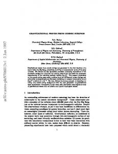
Apr 1, 2010 - A schematic view of two loops of cosmic strings in collision is shown in Fig. 1 . After collision, there are four junctions and eight kinks.
Cosmic Strings Collision in Cosmological Backgrounds Hassan Firouzjahi1 ,∗ Salomeh Khoeini-Moghaddam1,2 ,† and Shahram Khosravi2,3‡ 1
School of Physics, Institute for Research in Fundamental Sciences (IPM), P. O. Box 19395-5531, Tehran, Iran
arXiv:1004.0068v1 [hep-th] 1 Apr 2010
2
Department of Physics, Faculty of Science,
Tarbiat Mo’allem university, Tehran, Iran and 3
School of Astronomy, Institute for Research in Fundamental Sciences (IPM), Tehran, Iran (Dated: April 2, 2010)
Abstract The collisions of cosmic strings loops and the dynamics of junctions formations in expanding backgrounds are studied. The key parameter controlling the dynamics of junctions formation, the cosmic strings zipping and unzipping is the relative size of the loops compared to the Hubble expansion rate at the time of collision. We study analytically and numerically these processes for large super-horizon size loops, for small sub-horizon size loops as well as for loops with the radii comparable to the Hubble expansion rate at the time of collision. PACS numbers:
∗ † ‡
Electronic address: firouz(AT)ipm.ir Electronic address: skhoeini(AT)tmu.ac.ir Electronic address: khosravi(AT)ipm.ir
1
I.
INTRODUCTION
In models of brane inflation cosmic strings are copiously produced [1, 2], for reviews see e.g. [3–7]. These cosmic superstrings are in the forms of fundamental strings (F-strings), D1-branes (D-strings) or the bound states of p F-strings and q D-strings, the (p, q) strings. When two (p, q) cosmic superstrings collide junctions are formed due to charge conservation. This is in contrast to the collision of conventional gauge strings where upon collision they exchange partners and intercommute with the probability close to unity. Therefore one may consider the junction formation as a novel feature of a network of cosmic superstrings which may prove crucial in cosmic superstrings detection in cosmological observations. Networks of cosmic strings with junctions have interesting physical properties, such as the formation of multiple images [8, 9] and non-trivial gravitational wave emission [10, 11]. Different theoretical aspects of (p, q) string construction were studied in [12–17] while the cosmological evolution of a string network with junctions has been investigated in [18]. In a recent paper [19] the collision of two loops of cosmic strings in a flat background was studied. It was found that with appropriate initial conditions determined by the angle of collision, the colliding loops velocities and the loops relative tensions, junctions can form. However, after the junction is formed it can not grow indefinitely and after some time the junction start to unzip and the colliding loops disentangle and pass by from each other. The junctions’ zipping and unzipping are interesting and yet non-trivial dynamical properties. These phenomena becomes more significant in the light of cosmic strings simulation by Urrestilla and Vilenkin [20]. In their model, the cosmic strings are two types of U(1) gauge strings with interactions between them. Due to the interaction, the strings cannot exchange partners and a bound state will form if the strings are not moving too fast. It was shown that the length and the distribution of the string network are dominated by the original strings and there is a negligible contribution to the string network length and population from the bound states strings. This can be understood based on the following two reasons. Firstly, the junctions may not form if the colliding strings are moving very fast so they can simply pass through each other [21–27]. Secondly and more interestingly, if the junctions are formed, they start to unzip during the evolution. Our aim here is to generalize the results of [19] to the case of cosmic strings loops collision in cosmological backgrounds, i.e. the radiation and the matter dominated era. As we shall 2
see in sections III and IV, the size of the loops compared to the Hubble radius at the time of collision plays a significant role in junctions evolutions and cosmic strings zipping and unzipping. The paper is organized as follows. In section II we present our set up and provide the formalism of junction formation for arbitrary cosmic strings loops colliding in cosmological backgrounds. This is a generalization of [22] and [28] where they presented the formalism of cosmic strings collision in the flat background. In section III we concentrate to the example of two identical loops in cosmological backgrounds. After setting the background equations for the loops profiles, we present the equations governing the dynamics of the junctions. For the case of very large loops (super-horizon size loops) and very small loops (sub-horizon size loops) we are able to present some analytical results. In section IV we present our full numerical results for different loop configurations. The conclusion is given in section V
II.
LOOPS COLLISION IN AN EXPANDING UNIVERSE
Here we present the formalism of junction formation for arbitrary cosmic strings loops colliding in a cosmological background. In section III we employ the results obtained in this section to the particular example of two identical loops at collision in cosmological backgrounds. The formalism of cosmic strings collision in a flat background was studied in [22] and [28]. Our cosmological background is the standard FRW metric ds2 = a2 (τ )(dτ 2 − dx2 ) ,
(1)
where τ is the conformal time related to the cosmic time t via dt = adτ , a(τ ) is the scale factor and we assume that the background space-time has no spatial curvature. Our cosmological background is either radiation dominated (RD) or matter dominated (MD). Suppose Xiµ represents the profile of the i-th cosmic string in the target space-time. As usual, we can go to the temporal gauge where the time on the string world-sheet is the same as the conformal time, X 0 = τ , and Xiµ = (τ, xi ). Denoting the other coordinate of the world-sheet parameterization by σ, the gauge condition x˙ i · x′i = 0 ,
(2)
holds where the · and the prime indicate the derivatives with respect to τ and σ respectively. 3
A schematic view of two loops of cosmic strings in collision is shown in Fig. 1 . After collision, there are four junctions and eight kinks. The formation of the kinks is a manifestation of the fact that the speed of light is finite and parts of the old strings which did not “feel” the formation of junctions evolve as before. In the following we denote the incoming strings by xi where i = 1, 2 whereas the newly formed strings are denoted by ya where a = 1, 2, 3. The junctions and the kinks on each string are described by σa = sa (τ ) and σi = ωi (τ ) respectively. As mentioned in [19, 28] one complexity of dealing with loops in collision is the orientation of the σi coordinate at junctions. We follow the prescription of [28] and use the sign parameterization for δaJ according to which δaJ can take values ±1. If the value of σa of a
particular string increases(decrease) towards the junction J, we assign δaJ = +1(δaJ = −1). With this prescription, the two ends of a piece of string ending in two neighboring junctions
have opposite δ parameters. The arrows in Fig. 1 indicate this prescription. Since it is important for the later analysis, we now give the values of δaJ at each junction: δ1 = +1 δ1 = −1 δ1 = −1 δ1 = +1 D : δ2 = −1 C : δ2 = +1 B : δ2 = +1 A : δ2 = −1 δ3 = −1 δ3 = +1 δ3 = +1 δ3 = −1
(3)
Equipped with the δ-prescription, the action for the system of two loops in collision is
S = − − −
2 XX
2 X
i=1 2 X
i=1
µi
Z
µi
Z
i=1
− µ3 − µ3 +
J
Z
Z
dτ dσi a (τ ) 2
dτ dσi a (τ ) 2
dτ dσi a (τ )
dτ dσ3 a (τ ) dτ dσ3 a2 (τ )
3 Z XX
a=1 2 Z XX J
2
2
J
+
µi
Z
i=1
q
q
q
(1 − y˙ i2 ) yi′ 2 θ(δiJ (sJi (τ ) − σi )) θ(δiJ (σi − ωiJ (τ )))
q
(1 − x˙ 2i ) x′i 2 θ(δiA (ωiA (τ ) − σi )) θ(δiB (ωiB (τ ) − σi ))
q
(1 − x˙ 2i ) x′i 2 θ(δiC (ωiC (τ ) − σi )) θ(δiD (ωiD (τ ) − σi ))
C C (1 − y˙ 32 ) y3′ 2 θ(δ3A (sA 3 (τ ) − σ3 )) θ(δ3 (s3 (τ ) − σ3 )) D D (1 − y˙ 32 ) y3′ 2 θ(δ3B (sB 3 (τ ) − σ3 )) θ(δ3 (s3 (τ ) − σ3 ))
¯ J (τ )] dτ a2 (τ ) faJ · [ ya (sJa (τ ), τ ) − y dτ a2 (τ ) kJi · [ xi (ωiJ (τ ), τ ) − yi (ωiJ (τ ), τ ) ] 4
(4)
B M
µ3 µ1
D
µ2
C µ1 N
µ2
A
FIG. 1: A schematic view of the loops at the time of collision(left) and after collision (right). The arrows in the right figure indicate the directions in which the σi coordinate increases. We use the convention that on a loop σi runs counter clockwise. There are four junctions and eight kinks in total.
where J represents the junctions A, B, C and D collectively. Here faJ and kJi are Lagrange multipliers which enforce that at the kinks the newly formed strings and the old strings meet, xi (ωiJ (τ ), τ ) = yi (ωiJ (τ ), τ ) and on the junctions the three newly formed strings join ¯ J (τ ) where y ¯ J (τ ) represents the position of the junction J in target together ya (sJa (τ ), τ ) = y space. As described above, in our convention δiJ is +1 if σ increases towards the junction and -1 in the opposite case. ¯ aJ , respectively, results in Varying the action with respect to faJ , kJa and y ¯ J (τ ) ya (sJa (τ ), τ ) = y
(5)
xi (ωiJ (τ ), τ ) = yi (ωiJ (τ ), τ ) X faJ = 0 .
(6) (7)
a
Varying the action with respect to xi results in the following standard equations [29] for the segments of old strings extended between two nearby kinks which are not influenced by the junctions formations a˙ ∂ x′i ∂ (x˙ i ǫxi ) + 2 x˙ i ǫxi = ( ), ∂τ a ∂σ ǫxi 5
(8)
whereas matching the Dirac delta functions gives the following boundary conditions at the kinks σi = ωiJ (τ ) kJi
� � x′i J J J = µi x˙ i ǫxi ω˙ i δi + δ ǫxi i
,
σi = ωiJ (τ ) .
(9)
Here ǫi is defined by [29] ǫi ≡
s
x′2 i 1 − x˙ 2i
(10)
Similarly, varying the action with respect to ya results in the following equations for the newly formed strings stretched between a junction and the nearby kink ∂ a˙ ∂ yi′ (y˙ a ǫya ) + 2 y˙ a ǫya = ( ). ∂τ a ∂σ ǫyi
(11)
Now there are Dirac delta functions at the junctions σa = sJa (τ ) and the kinks (for strings 1 and 2) σi = ωiJ which result in the following boundary conditions � � yi′ J J J J , σi = ωiJ (τ ) δi ki = µi y˙ i ǫyi ω˙ i δi + ǫyi � � ya′ J J J J , σa = sJa (τ ) . δa fa = µa y˙ a ǫya s˙ a δa + ǫya
(12) (13)
Combining Eqs (7) and (13) result in X a
µa δaJ
� � ya′ J y˙ a ǫya s˙ a + = 0. ǫya
(14)
Eliminating kJi from Eqs. (9) and (12), and using the gauge condition (2), it is easy to show that ǫxi = ǫyi = ǫi
(15)
δiJ ω˙ iJ ǫi = −1
(16)
The solutions of the loops in cosmological backgrounds can not be expressed in terms of the the usual right- and left-movers. However, one can define the right- and left-momenta p± a as J
ya′ ± δaJ y˙ a ǫa x′ = i ± δiJ x˙ i ǫi
p± ya = J
p± xi
6
(17)
2
with p± a = 1. Starting with the time derivative of (5) x′ ω˙ iJ + x˙ i = y′ ω˙ iJ + y˙ i , J
(18)
J
one can show that p− yi = p− xi . This is the key formula which relates the unknown quantities J
J
− p− yi for the newly formed strings to the known quantities pxi from the old strings.
Starting with the time-derivative of Eq. (5) combined with Eq. (14) one obtains an − equation for p+ ya in terms of pyb J J J − δaJ (1 + δaJ ǫa s˙ Ja ) p+ ya = δa (1 − δa ǫa s˙ a ) pya −
2X µb δbJ (1 − δbJ ǫb s˙ Ja ) p− yb . µ ¯ b
(19)
2
Imposing the condition p± a = 1 one obtains qa − qa where µ ¯ a ≡ µa /¯ µ, µ ¯≡
P
a
X
µ ¯b qb cab +
b
X bc
µ ¯b µ ¯c qb qc cbc − 1 = 0
(20)
− µa , qaJ ≡ 1 − δaJ ǫa s˙ Ja and cab ≡ δaJ δbJ p− ya · pyb .
Now we provide an equation for the energy conversation at the junction. For this purpose, multiplying Eq (20) by µ ¯a and summing over a results in X a
µ ¯a qa −
X
µ ¯a µ ¯ b cab +
ab
X abc
µ ¯aµ ¯b µ ¯c qb qc cab − 1 = 0
(21)
However, with the reshuffling of the indices, one can easily check that the second and the third term above cancel out and one obtains X
µ ¯a qa = 1
(22)
δaJ µa ǫa s˙ a = 0 .
(23)
a
or
X a
This is a generalization of the case of strings in flat background studied in [22] corresponding to ǫa = 0. Defining cˆab = 1 − cab and using the energy conservation one can check that Eq. (20) results in qa
X
µ ¯b cˆab qb =
b
X bc
7
µ ¯bµ ¯ c cˆbc qb qc
(24)
Writing explicitly, and using (23), yields q1 (1 − 2¯ µ1 )(¯ µ2 q2 cˆ12 + µ ¯ 3 q3 cˆ13 ) = 2¯ µ2 µ ¯3 q2 q3 cˆ23
(25)
q2 (1 − 2¯ µ2 )(¯ µ1 q1 cˆ12 + µ ¯ 3 q3 cˆ23 ) = 2¯ µ1 µ ¯3 q1 q3 cˆ13
(26)
q3 (1 − 2¯ µ3)(¯ µ2 q2 cˆ23 + µ ¯1 q1 cˆ13 ) = 2¯ µ2 µ ¯ 1 q2 q1 cˆ12 .
(27)
Eliminating q3 and q2 from the first two equations above and plugging in (23) results in our main formula of interest 1 − δ1J ǫ1 s˙ J1 =
µ ¯M1 cˆ23 , µ1 [M1 cˆ23 + M2 cˆ13 + M3 cˆ12 ]
(28)
where M1 ≡ µ21 − (µ2 − µ3 )2 with a similar definition for M2 and M3 . One can also obtains a similar equation for s˙ 2,3 with an appropriate permutation of the indices. This set of equations for s˙ Ja is our starting point to study the evolutions of junctions.
III.
JUNCTION EVOLUTIONS
In previous section we have presented the general formalism of cosmic strings loops collision in a cosmological background. Here we specialize to the example of two identical loops at collision in a cosmological background where the analysis can be handled somewhat analytically. Before dealing with the loops in collision, here we summarize the background solutions for a loop in expanding background. Suppose the collision happens at the time τ = τ0 . One can check that the cosmic time t and the conformal time τ are related by t = τ n+1 /τ0n (n + 1) where we have considered a power law expansion for the scale factor a(τ ) = (τ /τ0 )n . For a radiation an matter dominated universe, n = 1, 2 respectively. In this convention, the scale factor at the time of collision is equal to unity. Also, calculation the Hubble expansion rate, H = da/a dt, one can check that the Hubble expansion rate at the time of collision is H0 = n/τ0 . Consider a loop extended in x − y plane moving relativistically in z direction. We choose the following ansatz for the loop configuration f (τ ) cos Rσ0 x = f (τ ) sin Rσ 0 z(τ ) 8
.
(29)
In this picture, R(τ ) ≡ a(τ )f (τ ) is the physical radius of the loop and R0 = f (τ0 ) represents the size of the loop at the time of collision. The independent equations of motions are 2n ′ F (1 − v 2 − F ′2 ) + (1 − v 2 − F ′2 )F −1 = 0 x 2n v(1 − v 2 − F ′2 ) = 0 . v′ + x
F ′′ +
(30) (31)
Here the loop center of mass velocity is defined by v = z(τ ˙ ). For the ease of the numerical investigations, we introduced the dimensionless time variable x ≡ τ /τ0 and F (x) ≡ f (τ )/τ0 . Also the prime here and below represents derivatives with respect to the dimensionless time x. This definition leads to F = f H0 /n which has a simple physical interpretation as follows. In our convention a(x) = xn , so at the time of collision, corresponding to x = 1, a = 1. The physical radius of the loop at the time of collision therefore is R0 = f (x = 1). Therefore, the initial condition F (x = 1) = f (x = 1)H0 /n is a measure of the physical radius of the loop compared to the Hubble radius at the time of collision. For Loops of super-horizon size at the time of collision F (x = 1) > 1, whereas for small sub-horizon sized loops at the time of collision F (x = 1) < 1. In the following, to simplify the notation we set F (x = 1) ≡ F1 . In general it is not easy to find analytical solutions for the set of equations (30) and (31). We solve this equation numerically. Our goal is to calculate cˆab for the loop with ansatz (29) and then obtain the evolution of junctions s˙ Ja . However, one may get some useful analytical information in some certain limits. These include very large super-horizon size loops at the time of collision (F1 ≫ 1) and small sub-horizon size loops (F1 ≪ 1). The collisions of loops in Minkowski background was studied in [19]. Here we generalize that study to the case of strings loops collision in an expanding background. In order to simplify the analysis, we consider the symmetric case where the two incoming loops have equal tension and physical radius at the time of collision. We assume that the loops are extended in x − y plane and are moving along the z-direction with velocity ±v. A schematic view of this example is given in Fig. 1 . By symmetry the newly formed string 3 will be static extended either along x or y directions. Whether it is a x-link or a y-link junction depends on the angle of collision α [22]. For small enough angle of collision it is a y-link while for a large enough angle of collision it would be an x-link junction. To be be specific, we consider a y-link junction where the string 3 is extended along the y-direction. 9
The profiles of the colliding loops are given by ∓b + f (τ ) cos Rσi0 xi = f (τ ) sin Rσi0 ±z(τ )
(32)
where for i=1 (i=2) we choose upper sign (lower sign). Here 2b is the impact factor. J
J
− From the continuity of the left moving momenta one has p− yi = pxi which can be served J
to find p− yi . From (17) we have J
− p− yi = pxi
J
J
√ − 1 − F ′2 − v 2 sin Rσi0 − δiJ F ′ cos Rσi0 √ = 1 − F ′2 − v 2 cos Rσi − δiJ F ′ sin Rσi 0 0 J ∓δi v(τ ) J
(33)
− J J J Using cˆJab ≡ 1 − δaJ δbJ p− ya · pyb at each junction and the fact that δ1 = −δ2 = −δ3 , one
obtains cˆJ11 = cˆJ22 = cˆJ33 = 0
(34) √ ′
cˆJ12 = 1 + v 2 − (1 − 2F ′2 − v 2 ) cos 2S1J + 2δ1J F 1 − F ′2 − v 2 sin 2S1J √ cˆJ13 = 1 + 1 − F ′2 − v 2 cos S1J − δ1J F ′ sin S1J √ cˆJ23 = 1 − 1 − F ′2 − v 2 cos S2J − δ1J F ′ sin S2J √ cˆJ23 + cˆJ13 = 2 + 2 1 − F ′2 − v 2 cos S1J − 2δ1J F ′ sin S1J
(35) (36) (37) (38)
Here and below, to simplify the notation the definition SaJ ≡ sJa /R0 is introduced. We
note that SaJ is dimensionless which is more suitable for numerical analysis. To obtain ′
′
Eqs. (35-37) we note that due to symmetry in problem, one has S1J = −S2J at each
junction J. On the other hand, one also observes that S1B (x = 1) + S2B (x = 1) = π and S1A (x = 1) + S2A (x = 1) = 3π which was used to simplify the final results in Eqs. (35-37). Plugging cˆab in our master equation (28), the evolution of the junction is given by J
S3′ =
c13 + cˆ23 ) − κ cˆ12 δ3J (κ − 1)(ˆ , F1 (κ − 1)(ˆ c13 + cˆ23 ) + cˆ12
(39)
where the dimensionless parameter κ is given by the ratio of the tensions κ ≡ 2µ1 /µ3. Also from the energy conservation Eq. (23) one has J
S1′ =
F1 √ J 1 − F ′2 − v 2 S3′ . κF 10
(40)
Equations (39) and (40) jointly can be used to solve for S3′ J . Due to symmetries involved in the problem, we only need to find the evolution of junctions B and D and the evolutions of junctions A and C are mirror images of junctions B and D. We note that the conditions for the junction formation is that the string 3 stretching between junctions B and D to be created. This requires that its length to increase initially with time: S3′ > 0 where S3 ≡ S3B − S3D measures the length of string BD. As we shall see in our numerical results, ′
′
usually this is translated into S3B > 0 and S3D < 0. However, in some very fine-tuned ′
′
situations one can also find examples where S3B > 0 and S3D > 0 such that S3′ > 0 is still satisfied. As explained in [19], after the junction formation, the entangled loops start to unzip. The onset of unzipping at junction J happens when S3′ J vanishes and changes its sign. As we shall see later, the unzipping times for junctions B and D are not equal. Since we are mainly interested in the evolution of the newly formed string BD, we define the onset of unzipping for string BD when S3 reaches a maximum and S3′ = 0. After that the length of string BD reduces with time. Sometime after unzipping, the loops disentangle from each other and pass by in opposite directions. The time of loops disentanglement happens when the junctions B and D meet corresponding to S3 = 0. However, we also encounter examples where the loops shrink to zero before they disentangle from each other. As explained above, the onset of unzipping at junction J is determined when S3′ J = 0. Here we show that the denominator in Eq. (39) is always positive so the sign of S3′ J is p controlled by the numerator of the above expressions. To see that note that − p2 + q 2 ≤ p p cosθ + q sin θ ≤ p2 + q 2 for real numbers p and q and arbitrary angle θ. Using these √ inequalities, one can easily check that cˆ12 ≥ 2v 2 and cˆ13 + cˆ23 ≥ 2(1 − 1 − v 2 ). On the other hand, as described in [22], one also requires that 2µ1 > µ3 for the junction formation to be allowed kinematically. In conclusion the denominator in S3′ J expression is always positive and the sign of S3′ J evolution is determined by the numerator of the above expressions. This plays important rules in determining the junctions unzipping times in the following discussions. As explained before, our goal is to solve the background loop equations (30) and (31) and use the resulting values of F (x) and v(x) in cˆab expressions to find the junctions evolutions from Eq. (39). This procedure can be done only numerically because both F (x) and v(x) can not be found analytically in general. Before presenting our full numerical analysis, we 11
consider two different limits where some analytical insights can be obtained for the junctions evolutions.
A.
Large super-horizon size loops
Here we consider the limit where the colliding loops are much larger than the Hubble radius at the time of collision, F1 ≫ 1. For the super-horizon size loops, one expect that they
are conformally stretched as the universe expands, R(τ ) ∝ a(τ ), where F ′ and F ′′ are small compared to unity. We will demonstrate this in our numerical analysis. Due to damping effects from the expanding background, the super-horizon loops become non-relativistic and v ≪ 1. In this approximation, one can easily solve the background equations (30) and (31) . Denoting F = F1 + ∆ where ∆ represents the small evolution of F , one obtains 2 1 ∆′′ + ∆′ + ≃ 0, x F1 which after neglecting the sub-dominant term, results in ∆≃−
x2 2(1 + 2n)F1
,
F′ ≃ −
x . (1 + 2n)F1
(41)
As the universe expands, the loop reenter the horizon in its subsequent evolutions. This can be approximated when ∆ ≃ −F1 which results in the time of the loop horizon reentry x∗ x∗ ≃
p 2(1 + 2n)F1 .
(42)
Our full numerical analysis, as we shall see in next section, verify that this is indeed a good approximation. From this expression for x∗ we see that with similar initial conditions, it takes longer for the loops to reenter the horizon in a matter dominated era as compared to the radiation dominated era. As the super-horizon size loops stretches conformally, its center of mass velocity reduces rapidly. For time smaller than x∗ one can find an approximate solution for v(x). Neglecting the terms containing v 2 and F ′2 in Eq. (31) one obtains v ′ + 2n v/x ≃ 0 which easily can be solved to give v(x) ≃ 12
v1 , x2n
(43)
where v1 is the value of v(x) at the time of collision, v1 ≡ v(x = 1). As explained above, we see that the loop central mass velocity reduces rapidly with time. We also see that for the matter dominated background with n = 2, the loss of velocity is more pronounced as compared to the radiation dominated background with n = 1. For the super-horizon size loops and keeping only terms up to F ′ in cˆab and neglecting F ′2 and v 2 as explained above, one obtains cˆ12 ≃ 1 − cos 2S1J + 2δ1J F ′ sin 2S1J
cˆ13 + cˆ23 ≃ 2 + 2 cos S1J − 2δ1J F ′ sin S1J
,
Plugging these into S3′ J expression results in
J S3′
� � � δ3J 1 + cos S1J κ cos S1J − 1 − δ1J F ′ sin S1J κ − 1 + 2κ cos S1J ≃ . F1 (1 + cos S1J ) (− cos S1J + κ) − δ1J F ′ sin S1J (κ − 1 − 2 cos S1J )
(44)
At the time of collision, one can neglect the terms containing F ′ in above expression and for small x one obtains ′
S3B (x ≃ 1) ≃ ′
δ3J κ cos S1J − 1 . F1 κ − cos S1J
(45)
For the junction to form we need S3B (x = 1) > 0. With S1B (x = 1) = α, the condition for junction formation is translated into 0 ≤ α ≤ αc
,
αc = arccos(κ−1 ) .
(46)
Interestingly, this is identical to the bound obtained in [23] for straight strings in collision at the small velocity approximation. This is expected, since the super-horizon size loops can be locally well approximated by the straight strings. Our full numerical analysis, presented in next section, indeed show that the bound on αc given by the above equation works very accurately for the large loops. As time goes by, the terms containing F ′ in Eq. (44) becomes important. We note that the denominator in Eq. (44) is positive so the sign of S3J evolution is determined by the numerator of Eq. (44). Consider junction B for example. For the junction B to unzip, S3B should slow down, requiring that the term containing F ′ in numerator of Eq. (44) gives a negative contribution. With δ1B = −1 and F ′ < 0 the F ′ correction in numerator of Eq. (44) indeed contributes negatively. This indicates that as time goes by, the rate of evolution of S3B slows down until S3′ B = 0 when the junction B starts to unzip. Similar argument applies to junction D too. 13
B.
Small sub-horizon size loops
Now we consider the limit where the colliding loops are much smaller than the Hubble radius at the time of collision, F1 ≪ 1. In this limit, the damping terms in Eqs. (30) can be neglected [29] and the loop evolution is the same as in the flat background. In this limit v is nearly constant and the loop has a simple periodic profile � � x−1 F (x) ≃ F1 cos , (47) γF1 √ where γ = 1/ 1 − v 2 is the Lorentz factor. To simplify the analysis, here we chose the initial
configuration such that F ′ = 0 at the time of collision. Neglecting the effects of expansion,
one would expect the criteria for zipping, unzipping and the loops disentanglement would be similar to cosmic strings loops collision in a flat background studied in [19]. Starting from the energy conservation formula (40), one obtains B(D)
B(D)
S1
=
S3 κγ
+ α.
(48)
Also calculating cˆab yields cˆ12 cˆ12 + cˆ13
� −1 + = 2 − 2γ cos γF1 � � −1 J Jx−1 = 2 + 2γ cos S1 + δ3 . γF1 2
−2
�
S1J
x δ3J
(49)
Plugging these in S3′ J expression yields S3′
J
� δJ (x−1) + 3 γF1 + α − γ � �. = F1 κγ − cos S3B + δ3J (x−1) + α κγ γF1 δ3J
κ cos
�
S3B κγ
(50)
The details of the loops zipping, unzipping and disentanglement were studied in [19]. Here we briefly outline the main results. For the junctions to form one requires that 0 < α < αc where αc = arccos(γ/κ). The unzipping times for junctions B and D, xuD and xuB , satisfy
xuD
−
xuB
� −2 −1
= 2γαF1 1 − κ
� � 1 sin α . 1− κγ α
(51)
Since sin α/α and 1/κγ are always less than unity, one concludes that xuD > xuB , indicating that the junction B which holds the external large arcs unzip sooner than the junction D 14
FHxL
vHxL
100
0.20
80 0.15
60 40
0.10
20
100
200
300
400
0.05
x
-20 2
4
6
8
10
x
FIG. 2: Here the background evolution of Eqs. (30) and (31) are presented with F1 = 100, v1 = 0.2 and F ′ (x = 1) = 0.1. The left figure shows F (x) whereas the right figure represents v(x). The solid lines are for the radiation dominated backgrounds (n = 1) and the dashed lines are for the matter dominated backgrounds (n = 2). We are considering the loops evolution until they shrink, i.e. until the first root of F (x) = 0.
which holds the internal smaller arcs. Although we have proved this only for small subhorizon loops but our numerical analysis show that this conclusion holds true in general. The loops disentangle at the time xf when S3 = 0, which is given by the parametric relation −1
κγ cos
Γ − cos
�
xf − 1 γF1
where Γ≡
�
"
√
1 − Γ2 − κγ µ1 α + sin α = 0 ,
(xf − 1)
κF1 sin(
xf −1 ) γF1
#
(52)
.
This is an implicit equation for xf which should be solved in terms of κ, γ, α and F1 . For this to make sense, we demand that xf − 1 < γF1 π/2 before the loops shrink to zero. IV.
NUMERICAL ANALYSIS
In this section we present our full numerical results for different loops configurations. To be specific, we consider three examples of (a): large super-horizon size loops with F1 = 100, (b): intermediate size loops with F1 = 0.5 and (c): small sub-horizon size loops with F1 = 0.01.
15
S3 Length of S3
50
100
150
200
250
x 0.5
-0.2
-0.4
50
100
150
200
250
x
-0.6 -0.5
-0.8 -1.0
FIG. 3: In these plots we have presented the evolution of junctions B and D for F1 = 100, α = π/9 and κ = 1.2. In the left figure the upper solid red curve represents S3B whereas the lower solid blue curve is that of S3D for the radiation dominated background. The dashed curve represents the corresponding curves in the matter dominated background. The right graph represents the length of the newly formed strings µ3 , S3 ≡ S3B − S3D . The solid (dashed) curve is for the radiation (matter) dominated background. We see that in both backgrounds, after junction formation, the string BD reaches a maximum length and get unzipped. However, only in the radiation dominated background S3 becomes zero before loops shrink indicating the loops disentanglement.
A.
Large super-horizon size loops
For super-horizon size loops with F1 ≫ 1 one expects that the loops are conformally stretched until they re-enter the horizon. In this period, the loops lose much of its center of mass velocity as demonstrated by Eq. (43). As mentioned before, the loss of velocity is more significant for the matter dominated backgrounds. Also from Eq. (42) we see that it takes longer for the loop to shrink for the matter dominated backgrounds as compared to the radiation dominated backgrounds. Both of these analytical conclusions were verified in our full numerical investigations. In Fig.2 we have presented the background solutions of F (x) and v(x) solving Eqs. (30) and (31) numerically. As is clear from the figure, in a matter dominated background, it takes longer for the loop to shrink. This in turn plays some roles in the junctions evolutions and loops disentanglement. In Fig.3 we have presented the evolutions of junction B and D solving Eq. (39) numerically. The left figure shows the evolution of junctions B and D both for matter and radiation dominated backgrounds. The
16
FHxL
vHxL 0.20
0.4 0.15
0.2 0.10
1.5
2.0
2.5
3.0
x 0.05
-0.2
x 1.5
FIG. 4:
2.0
2.5
3.0
Here the background evolution for F (x) and v(x) are presented with F1 = 0.5, v1 =
0.2, F ′ (x = 1) = 0.1. The solid (dashed) curves are for the radiation (matter) dominated backgrounds.
right figure shows the length of the newly formed string µ3 stretching between junctions B and D which is S3 ≡ S3B − S3D . As mentioned previously for the junction to form we require
that S3′ > 0. Form the right figure we see that the junction is created in both cosmological backgrounds. After the junction formation, S3 reaches a maximum value indicating the unzipping of the newly formed strings BD. After this time, S3 reduces. When S3 = 0 the junctions B and D meet again and the loops disentangle and pass by from each other. From the right figure we see that for the radiation dominated background the loops disentanglement indeed take place. However, for the matter dominated background, we see that before loops find the opportunity to disentangle, they shrink to zero. As explained below Eq. (51) the junction B unzips sooner than junction D which is also demonstrated in the left figure of Fig. 3.
B.
Loops with intermediate sizes
For the loops with the sizes comparable to the Hubble radius at the time of collision, F1 ∼ 1, we can only do numerical analysis. On the physical grounds one expects that the evolution of F (x) and v(x) is less sensitive to the background cosmological expansion as compared to large super-horizon size loops. In Fig. 4 we have presented the background evolution of F (x) and v(x) for F1 = 0.5. As expected v(x) changes slowly and F (x) evolves similarly for both matter and radiation dominated backgrounds. In Fig. 5 we have presented 17
S3 Length of S3
1.2
1.4
1.6
1.8
x
-0.1
0.4
0.2
-0.2 1.2
-0.3 -0.4
-0.2
-0.5
-0.4
1.4
1.6
1.8
x
-0.6
FIG. 5: Here we present the evolutions of junctions B and D and the string BD for F1 = 0.5, α = π/9 and κ = 1.2. In the left figure the upper solid red curve represents S3B whereas the lower solid blue curve is that of S3D for the radiation dominated background. The dashed curves represent the corresponding curves in the matter dominated background. The right graph represents the length of the newly formed string BD, S3 . The solid (dashed) curve is for the radiation (matter) dominated background. We see that in both backgrounds, after junction formation, the string BD reaches a maximum length and get unzipped. We also observe that the onsets of string BD unzipping and the loops disentanglement happen sooner in a radiation dominated era.
the evolutions of junctions B, D and the string BD . For both radiation dominated and matter dominated backgrounds we see that the junctions are formed followed by the string BD unzipping and the loops disentanglement. One observes that the onsets of string BD unzipping (when S3 reaches a maximum) and also the loops disentanglement happen earlier for the radiation dominated era as compared to the matter dominated era. This may be interpreted by noting that for the radiation dominated backgrounds the loops reenter the horizon and shrink sooner as can be seen qualitatively from Eq. (42).
C.
Small sub-horizon size loops
For small loops, F1 ≪ 1, as explained before one expects the background cosmological evolutions do not play important roles. We have presented the analytical results for small loops in subsection III B. In Fig. 6 we have presented the full numerical solutions of F (x) and v(x). As expected F (x) shows simple periodic behavior and v(x) does not change much
18
FHxL
vHxL
0.010
0.20
0.005
0.15
x 1.005
1.010
1.015
1.020
1.025
0.10
1.030 0.05
-0.005
1.005
-0.010
1.010
1.015
x
FIG. 6: Here the solutions of F (x) and v(x) for both matter dominated and radiation dominated backgrounds are shown for F1 = 0.01, v1 = 0.2 and F ′ (x = 1) = 0. As expected, the background cosmological evolutions do not play important roles so F (x) indicates simple periodic behavior and v(x) changes slowly.
in each period. In Fig. 7 we have presented the junctions evolution. As expected, the junctions evolutions are identical for bath matter and radiation dominated backgrounds. We also observe that the string BD unzipping and the loops disentanglement take place in this example. As demonstrated analytically in Eq. (51) the junction B unzips sooner than junction D which is also demonstrated in the left figure of Fig. 7.
V.
CONCLUSION
In this work we have studied the cosmic strings collision in cosmological backgrounds. After presenting the general formalism in section II we have concentrated to the example of colliding loops. The motivation for this work was to understand analytically the findings of simulation in [20] where it was found that there were little contributions from the bound states strings in their multiple strings network. One can understand this phenomena as follows. For the junctions to develop upon strings collision, some appropriate initial conditions should be satisfied. These depends on the relative tensions of the colliding strings, the angle of collision and their relative velocities. Yet the more interesting observation is that even when junctions are created, they can not grow indefinitely and the bound state strings start to unzip.
19
S3
Length of S3
1.005
1.010
1.015
x
0.2
1.005
-0.2
1.010
1.015
x
-0.2
-0.4 -0.4
-0.6
-0.6 -0.8
FIG. 7: Here the junctions evolutions are shown for F1 = 0.01, α = π/9 and κ = 1.2. In the left figure, the upper red (lower blue) curve shows S3B (S3D ). Interestingly the curves corresponding to the radiation and the matter dominated backgrounds coincide to each other. As demonstrated by Eq. (51) the junction B unzip sooner than the junction D. The right figure shows the length of string BD given by S3 . Again the curves corresponding to the matter dominated and the radiation dominated backgrounds coincide.
As described in [19], for straight cosmic strings at collision the junctions do not unzip once they are materialized. However, for colliding loops in a flat background the zipping and unzipping generically happen [19]. The natural question is how sensitive are these results to the expansion of the Universe. Here we find some interesting results indicating that the background expansion plays important roles in strings zipping, unzipping and their eventual disentanglement . The key parameter here is the relative size of the loops compared to the Hubble expansion rate at the time of collision. For large super-horizon size loops one may approximate them with straight strings. This implies that if junctions are formed upon loops collision it will grow initially as in straight strings examples. However, as the Universe expands the loops stretch conformally until they re-enter the Horizon. Meanwhile their velocities reduces rapidly. The net effect is that the rate of bound state strings creation slows down until it starts to unzip. Eventually the loops disentangle from each other and pass by from each other in opposite directions if they did not shrink to zero by then. On the other hand, for small sub-horizon size loops one can neglect the effects of the expansion and the results of [19] holds true. The case of colliding loops with the sizes comparable to the Hubble radius at the time of collision is more non-trivial which shares some features with 20
small and large loops cases. Our numerical investigations also show that the junction formation and the zipping and unzipping phenomena are sensitive to the angle of collision α and the strings relative tensions parametrized by κ. It would be interesting to study these phenomena in the multi parameter space of F1 , κ and α. Also to simplify the analysis, we have restricted ourselves to the example of coplanar colliding loops with equal tensions and radii. It would be interesting to study the general case where the loops have different sizes and orientations and there are hierarchies between the sizes of the loops and the Hubble expansion rate at the time of collision.
Acknowledgments
We would like to thank Tom Kibble for useful discussions and comments.
References
[1] S. Sarangi and S. H. H. Tye, “Cosmic string production towards the end of brane inflation,” Phys. Lett. B 536, 185 (2002) [arXiv:hep-th/0204074]. [2] M. Majumdar and A. Christine-Davis, “Cosmological creation of D-branes and anti-D-branes,” JHEP 0203, 056 (2002) [arXiv:hep-th/0202148]. [3] E. J. Copeland and T. W. B. Kibble, “Cosmic Strings and Superstrings,” Proc. Roy. Soc. Lond. A 466, 623 (2010) [arXiv:0911.1345 [hep-th]]. [4] S. H. Henry Tye, “Brane inflation: String theory viewed from the cosmos,” Lect. Notes Phys. 737, 949 (2008) [arXiv:hep-th/0610221]. [5] T. W. B. Kibble, “Cosmic strings reborn?,” astro-ph/0410073. [6] A. C. Davis and T. W. B. Kibble, “Fundamental cosmic strings,” Contemp. Phys. 46, 313 (2005) [arXiv:hep-th/0505050]. [7] M. Sakellariadou, “Cosmic Superstrings,” arXiv:0802.3379 [hep-th]. [8] B. Shlaer and M. Wyman, “Cosmic superstring gravitational lensing phenomena: Predictions for networks of (p,q) strings,” Phys. Rev. D 72, 123504 (2005) [arXiv:hep-th/0509177].
21
[9] R. Brandenberger, H. Firouzjahi and J. Karouby, “Lensing and CMB Anisotropies by Cosmic Strings at a Junction,” Phys. Rev. D 77, 083502 (2008) [arXiv:0710.1636 [hep-th]]; T. Suyama, “Exact gravitational lensing by cosmic strings with junctions,” Phys. Rev. D 78, 043532 (2008) [arXiv:0807.4355 [astro-ph]]. [10] R. Brandenberger, H. Firouzjahi, J. Karouby and S. Khosravi, “Gravitational Radiation by Cosmic Strings in a Junction,” JCAP 0901, 008 (2009) [arXiv:0810.4521 [hep-th]]; M. G. Jackson and X. Siemens, “Gravitational Wave Bursts from Cosmic Superstring Reconnections,” JHEP 0906, 089 (2009) [arXiv:0901.0867 [hep-th]]; P. Binetruy, A. Bohe, T. Hertog and D.A. Steer, “Gravitational Wave Bursts from Cosmic Superstrings with Y-junctions, ” arXiv:0907.4522. [11] L. Leblond, B. Shlaer and X. Siemens, “Gravitational Waves from Broken Cosmic Strings: The Bursts and the Beads,” arXiv:0903.4686 [astro-ph.CO]. [12] E. J. Copeland, R. C. Myers and J. Polchinski, “Cosmic F- and D-strings,” JHEP 0406, 013 (2004), hep-th/0312067 ; G. Dvali and A. Vilenkin, “Formation and evolution of cosmic D-strings,” JCAP 0403, 010 (2004) [arXiv:hep-th/0312007]; L. Leblond and S.-H. H. Tye, “Stability of D1-strings inside a D3-brane,” JHEP 0403, 055 (2004), hep-th/0402072; N. Barnaby, A. Berndsen, J. M. Cline and H. Stoica, “Overproduction of cosmic superstrings,” JHEP 0506, 075 (2005) [arXiv:hep-th/0412095]. [13] H. Firouzjahi, L. Leblond and S. H. Henry Tye, “The (p,q) string tension in a warped deformed conifold,” JHEP 0605, 047 (2006) hep-th/0603161; H. Firouzjahi, “Dielectric (p,q) strings in a throat,” JHEP 0612, 031 (2006) hep-th/0610130; K. Dasgupta, H. Firouzjahi and R. Gwyn, “Lumps in the throat,” JHEP 0704, 093 (2007) [arXiv:hep-th/0702193]; M. Lake, S. Thomas and J. Ward, “String Necklaces and Primordial Black Holes from Type IIB Strings,” arXiv:0906.3695 [hep-ph]. [14] M. G. Jackson, N. T. Jones and J. Polchinski, “Collisions of cosmic F- and D-strings,” JHEP 0510, 013 (2005), hep-th/0405229; A. Hanany and K. Hashimoto, “Reconnection of colliding cosmic strings,” JHEP 0506, 021 (2005) [arXiv:hep-th/0501031];
22
K. Hashimoto and D. Tong, “Reconnection of non-abelian cosmic strings,” JCAP 0509, 004 (2005) [arXiv:hep-th/0506022]; M. Eto, K. Hashimoto, G. Marmorini, M. Nitta, K. Ohashi and W. Vinci, “Universal reconnection of non-Abelian cosmic strings,” Phys. Rev. Lett. 98, 091602 (2007) [arXiv:hep-th/0609214]; M. G. Jackson,
“Interactions of cosmic superstrings,”
JHEP 0709,
035 (2007)
[arXiv:0706.1264 [hep-th]]. [15] H. Firouzjahi, “Energy Radiation by Cosmic Superstrings in Brane Inflation,” Phys. Rev. D 77, 023532 (2008) [arXiv:0710.4609 [hep-th]]. [16] Y. Cui, S. P. Martin, D. E. Morrissey and J. D. Wells, “Cosmic Strings from Supersymmetric Flat Directions,” Phys. Rev. D 77, 043528 (2008) [arXiv:0709.0950 [hep-ph]]. [17] A. C. Davis, W. Nelson, S. Rajamanoharan and M. Sakellariadou, “Cusps on cosmic superstrings with junctions,” arXiv:0809.2263 [hep-th]. [18] S. H. Tye, I. Wasserman and M. Wyman, “Scaling of multi-tension cosmic superstring networks,” Phys. Rev. D 71, 103508 (2005) [Erratum-ibid. D 71, 129906 (2005)] [arXiv:astro-ph/0503506]; L. Leblond and M. Wyman, “Cosmic necklaces from string theory,” astro-ph/0701427; A. Avgoustidis and E. P. S. Shellard, “Velocity-Dependent Models for Non-Abelian/Entangled String Networks,” arXiv:0705.3395 [astro-ph]; A. Rajantie, M. Sakellariadou and H. Stoica, “Numerical experiments with p F- and q Dstrings: the formation of (p,q) bound states,” arXiv:0706.3662 [hep-th]; M. Sakellariadou and H. Stoica, “Dynamics of F/D networks: the role of bound states,” JCAP 0808, 038 (2008) [arXiv:0806.3219 [hep-th]]. [19] H. Firouzjahi, J. Karouby, S. Khosravi and R. Brandenberger, “Zipping and Unzipping of Cosmic String Loops in Collision,” Phys. Rev. D 80, 083508 (2009) [arXiv:0907.4986 [hepth]]. [20] J. Urrestilla and A. Vilenkin, “Evolution of cosmic superstring networks: a numerical simulation,” JHEP 0802, 037 (2008) [arXiv:0712.1146 [hep-th]]. [21] L. M. A. Bettencourt and T. W. B. Kibble, “Nonintercommuting Configurations In The Collisions Of Type I U(1) Cosmic Strings,” Phys. Lett. B 332, 297 (1994) [arXiv:hep-ph/9405221]. [22] E. J. Copeland, T. W. B. Kibble and D. A. Steer, “Collisions of strings with Y junctions,”
23
Phys. Rev. Lett. 97, 021602 (2006) [arXiv:hep-th/0601153]. [23] E. J. Copeland, T. W. B. Kibble and D. A. Steer, “Constraints on string networks with junctions,” Phys. Rev. D 75, 065024 (2007) [arXiv:hep-th/0611243]. [24] E. J. Copeland, H. Firouzjahi, T. W. B. Kibble and D. A. Steer, “On the Collision of Cosmic Superstrings,” Phys. Rev. D 77, 063521 (2008) [arXiv:0712.0808 [hep-th]]. [25] P. Salmi, A. Achucarro, E. J. Copeland, T. W. B. Kibble, R. de Putter and D. A. Steer, “Kinematic Constraints on Formation of Bound States of Cosmic Strings - Field Theoretical Approach,” Phys. Rev. D 77, 041701 (2008) [arXiv:0712.1204 [hep-th]]. [26] N. Bevis and P. M. Saffin, “Cosmic string Y-junctions: a comparison between field theoretic and Nambu-Goto dynamics,” Phys. Rev. D 78, 023503 (2008) [arXiv:0804.0200 [hep-th]]. [27] A. Achucarro and R. de Putter, “Effective non-intercommutation of local cosmic strings at high collision speeds,” Phys. Rev. D 74, 121701 (2006) [arXiv:hep-th/0605084]. [28] N. Bevis, E. J. Copeland, P. Y. Martin, G. Niz, A. Pourtsidou, P. M. Saffin and D. A. Steer, “On the stability of Cosmic String Y-junctions,” arXiv:0904.2127 [hep-th]. [29] N. Turok and P. Bhattacharjee, “Stretching Cosmic Strings,” Phys. Rev. D 29, 1557 (1984).
24