Cosmological vector perturbations in vector-tensor ...

Cosmological vector perturbations in vector-tensor teories of gravitation. CMB anomalies R. Dale , J. A. Morales† and D. Sáez†


Departamento de Física, Ingenieria de Sistemas y Teoría de la Señal, Universidad de Alicante, 03690, San Vicente del Raspeig, Alicante, Spain † Departamento de Astronomía y Astrofísica, Universidad de Valencia, 46100, Burjassot, Valencia, Spain Abstract. Five years of CMB (cosmic microwave background) observations with WMAP (Wilkinson Microwave Anisotropy Probe) have pointed out some anomalies in the first CMB temperature multipoles. We have recently proved that large scale cosmological vector modes could explain both the alignments of the second and third multipoles and the planar character of the octopole; nevertheless, these modes decay in standard cosmology. Here, we compare the evolution of cosmological vector perturbations in a certain vector-tensor theory of gravitation with the standard evolution in the framework of General Relativity. The importance of the resulting differences –in order to explain CMB anomalies– is briefly discussed. Keywords: cosmology:theory–large-scale structure of universe–cosmic microwave background PACS: 04.50.Kd, 98.80.Jk, 98.70.Vc

INTRODUCTION Recently, superhorizon vector modes have been used (see [1] and [2]) to explain, in the framework of GR (general relativity), most of the anomalies observed in the cleaned WMAP (Wilkinson Microwave Background Probe) maps of the CMB (cosmic microwave background); however, subhorizon vector modes should be negligible to avoid  CMB anomalies at too small angular scales (too large values). In this paper, the evolution of vector perturbations with different spatial scales is studied in both GR and a certain vector-tensor (V-T) theory. The resulting evolutions are compared to point out that the V-T theory seems to be more appropriate to account for the CMB anomalies: (1) small quadrupole amplitude, (2) planar character of the octopole, (3) quadrupole-octopole alignment, and so on [3]. Along the paper, a, τ , z, and G stand for the scale factor, the conformal time, the redshift, and the gravitation constant, respectively. Greek (Latin) indexes run from 0 to 3 (1 to 3). Whatever function ξ may be, ξ  0  is its present value and ξ˙ its partial derivative with respect to τ . Quantity ρc is the critical energy density, ρr (ρm ) is the radiation (matter) energy density, and ρB  ρr  ρm is the total background energy density of the cosmological fluid. Units are defined in such a way that the speed of light is c  1. The present value of the scale factor, a  0  , is assumed to be unity (which is always possible  in flat universes) and, then, the relation a  1  z  1 is satisfied. The Einstein, Ricci, and metric tensors are G µν , Rµν , and gµν , respectively. The scalar curvature is R, the

symbol ∇α stands for the covariant derivative, and n is the unit vector defining the line of sight.

A VECTOR-TENSOR THEORY A Lagrangian involving four free parameters was presented in [4]. It depends on the metric and a vector field A µ and, consequently, it leads to a general V-T theory of gravitation. In the same reference, the field equations and the parametrized post-Newtonian (PPN) limit of the resulting V-T theory were given in terms of the free parameters. We have chosen a V-T theory based on the Lagrangian








16π G 

1

 R



η˜ Rµν Aµ Aν  γ˜ ∇ν Aµ ∇ν Aµ

(1)



with η˜  γ˜. Since the general Lagrangian considered by Will [4] can be easily reduced to the form (1), for appropriate values of the free parameters, the field equations and PPN limit of the theory corresponding to (1) can be easily calculated from those given in [4] (parameter particularization). Thus, it is found that the field equations of the theory based on Eq. (1) can be written as follows: (2) ∇ν ∇ν Aµ  Rµν Aν  0 Gµν In this last equation, Tµν vacuum, and A Tµν 







1 A (3) Rgµν  8π GTµν  Tµν 2 is the energy momentum tensor of radiation, matter and Rµν

 η˜   Sαβ Sααβ  12 S2  α  2Aβ ∇ α Sαβ  gµνα  2 Sµα Fν  Sνα Fµ  2 SSµν  A ∇α Sµν    

(4)

where 2Sαβ  ∇α Aβ  ∇β Aα , 2Fαβ  ∇α Aβ ∇β Aα , and S  Sαα . Equation (2) has been previously studied ([5], [6]). Its solutions generate the infinitesimal harmonic transformations. The PPN limit of the V-T theory obtained from the Lagrangian (1) appears to be the same as that of GR, excepting parameter α2 , which vanishes in GR but takes on the value α2  2η˜ A2 , where A2  Aµ Aµ , in the V-T case. Finally, in some V-T theories, the gravitational constant undergoes small variations, e.g., in the Will-Nordtvedt theory [7], the gravitational constant appears to be proportional to 1  A2 2  , namely, it is not a true constant; however, in the V-T theory we are studying, G is a true constant (as in GR). This fact is important to compare predictions and observations and, consequently, to bound the possible α2 values. Some aspects of the V-T theory based on the Lagrangian (1) have been recently studied. After proving that ρA is a form of dark energy for η˜ 0, the authors of paper [8] explained the SN Ia observations by assuming a density parameter ΩA 0 61 (without cosmological constant); nevertheless, in the same case, the CMB angular power spectrum has not been calculated and, moreover, although it is argued that the PPN limit of









the theory could be compatible with solar system observations, this compatibility has not been explicitly proved. We then prefer another version of the same V-T theory to develop our study about the evolution of vector perturbations; This version would explain the same observations as the ΛCDM concordance model. Actually, it is a modification of this model involving the vector field A µ of the V-T theory with a small density parameter ΩA 0 01, where the positive (negative) sign corresponds to η˜ 0 (η˜ 0). Values of ΩA smaller than 0 01 have been also considered. Evidently, low Ω A values ensure that the model explains the same cosmological observations as the concordance one. The main part of dark energy would be due to fields in the vacuum state, quintessence, and so on.

 






 



VECTOR PERTURBATIONS IN GENERAL RELATIVITY In standard cosmology, there are vector perturbations associated to: the peculiar velocity vi , the metric components hi  g0i , and the anisotropic stresses Πi j [9]. Condition Πi j  0 is assumed. Vectors h and v can be expanded in terms of the so-called fundamental vector har monics (basis), whose form is Q  ε exp ik r  , where k is the wavenumber vector (see [10]). A representation of vectors ε and ε is [1]:





ε1 



ε2 













  ik2   σ  2   k2 k3  k  ik1   σ  2 ε3   σ  k  2  k1 k3 k

(5) (6) (7)

where σ  k12  k22  1 2 . The expansions read as follows h  B Q  B Q and v  v Q  v Q . Functions   B k τ  and v k τ  describe the perturbation in momentum space. The differences    vc k τ   v k τ  B k τ  are gauge invariant. The components of the angular velocity in momentum space are [2]:

  









 

 



 

    ε  k   w  iv  ε  k  ε  k   w  iv  ε  k  ε  k   (8) In standard cosmology (with and without cosmological constant) the time variation of v  and B  are as follows [1]: (i) in the matter dominated era,       v  τ  k   v    k   a τ   B  τ  k   6H   Ω v    k   k a τ  (9) w1  ivc ε2 k3

3

2

2

c

3

1

1

3

3

c

1

2

1

2

c

c

2 0

c0

and, (ii) in the radiation dominated era,

 





vc τ k   vc τeq k   constant



B

  τ  k 

2 2

m c0





 



8ρr  0  vc τeq k  k2 a2 τ 



(10)

where, τeq stands for the conformal time at matter radiation equivalence. Quantities vc and, consequently, the angular velocity w are constant (decrease proportional to a 1 ) during the radiation (matter) dominated era. We see that, in GR, all the



scales evolve in the same way and, consequently, the subhorizon vector modes cannot decay fast than the superhorizon ones to reach the necessary domination of the superhorizon scales (see the introduction) ; this means that, in GR, this domination must arise as a result of some unknown process generating suitable vector perturbations. In other words, before evolution, the initial spectrum of vector perturbations must already have negligible (significant) power for subhorizon (superhorizon) scales. The most important contribution to the relative temperature variation produced by the superhorizon vector modes is [2]: ∆T 6H 20  Ωm T 

re



dr   F r r

a2

0

(11) 

where re is the radial coordinate at emission time (last scattering surface), F r    Fpq r  n p nq ,     kp vc  0  k  εq κ  exp ik r  d 3 k i (12) Fpq r   2 k













and κ  k k. Finally, the rotation of the polarization direction δ ψ (Skrotskii effect, see [1]) is

δ ψ  3H 20 Ωm where 

G r 

 

vc  0  ε



κ

re 0





vc  0  ε κ 



(13)



exp ik r  d 3 k

k







 dr  n G r  a2 r 








(14)

We see that, in GR, both ∆T T and δ ψ only depend on vc  0  k  . The same occurs with the angular velocity. We can then state that, in order to explain the CMB anomalies,  quantities vc  0  k  must be significant (negligible) for superhorizon (subhorizon) spatial scales (see above).



VECTOR PERTURBATIONS IN THE VECTOR-TENSOR THEORY The following equations:



 

h  B Q  B Q

 

vc  vc Q  vc Q



Πi j  0

(15)

are valid in GR, and they are also assumed in the V-T theory together with the new expansion A  A Q  A Q (16) 

 





 



  

where A  A1 A2 A3  and Aµ  A0 A  . The field equations of the theory couple the evolution of B , vc , A , and the variables A0 and a describing the background. Our universe has baryons, CDM, the field A µ , and

a cosmological constant. The density parameters of these components are assumed to be Ωb  0 04, Ωc  0 23, ΩA  0 01, and ΩΛ  0 73 0 01, respectively. Hence, our model is flat (Ωb  Ωc  Ωλ  ΩA  1) and very similar to the so-called concordance model. From Eqs. (2)–(4) one easily finds the equations describing the homogeneous and isotropic background, in which the line element is











ds2  a2





d τ 2  δi j dxi dx j  

(17)

  



and the vector field has the covariant components A0 τ  0 0 0  . The resulting equations are: a¨ A¨ 0  4 A0 (18) a 3



a˙2 8π G a2 ρB  η a2 



4a˙ ˙ A0 A0 a3




4a˙ a¨ a˙2 2  2  8π G  a2 pB  η 3 A0 A˙ 0 a a a





1 ˙2 A 2a2 0

where η  η˜ 8π G. From Eqs. (2)–(4), plus the perturbed line element ds2  a2





d τ 2  δi j dxi dx j 







3 ˙2 A 2a2 0

 



2a˙2 2 A a4 0 



2
2

a¨ a˙2 A2  a3 a4  0 

 

B Qi dxi d τ 





(19) (20)

(21)

and the perturbed vector field A µ  A0 τ  A Qi  , we have found the following equations describing –to first order– the evolution of vc , B , and A :

  2 aa¨ 



A¨  k2 A0 B 







32π Gη ˙ A0 2A0 B a2

a˙ B˙  2 B  a and





2

a˙2 a2







k2 A



(22)

  A   A  A B˙   A˙   

  

a2 B  16π G 2 ρB  pB vc k

 

0



η A0 A a2



0

A0 B

 

(23)

(24)

The system formed by Eqs. (18) to (20) and (22) to (24) can be written as a system of first order differential equations by using appropriate variables and, then, the new system can be numerically solved for suitable initial conditions. These conditions have been fixed in the radiation dominated era, at redshift z  108 . Close to the initial redshift, we have proved that, approximately, all the variables involved in the problem evolve as powers of τ . On account if this fact, we have found the growing, constant and decaying modes, and we have chosen consistent initial conditions. The evolution of quantity vc is given in Figs. 1–4, where dashed and solid lines correspond to GR and V-T, respectively. In the four cases we have fixed η  1, ΩA  0 01 and ΩΛ  0 74. The unique difference is that, in each case, the spatial scale L (k  2π L) is different. In Fig. 1, this scale is L  2  104 M pc (superhorizon











−14

10

V−T GR −16

10

−18

10

−20

vc+

10

−22

10

−24

10

−26

10

−28

10

8

6

10

10

4

10

2

0

10

−2

10

z

10

−4

10

FIGURE 1. Superhorizon spatial scale with k 2π L and L 2 104 M pc. Solid line (V-T) shows a growing small vc value; however, dashed line (GR) exhibits a decreasing vc coefficient proportional to a 1.










2.0 V−T GR 1.5

vc+ × 1018

1

0.05

0

−0.5

−1 8 10

6

10

4

10

2

0

10

−2

10

z

10

−4

10

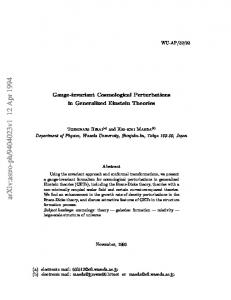
FIGURE 2. Subhorizon large spatial scale with k 2π L and L 2 103 M pc. Solid line (V-T) shows a vc value oscillating around the dashed line (decaying mode of GR: v c ∝ a 1 )










1.5 V−T GR 1

vc+ × 1019

0.5

0

−0.5

−1

−1.5 8 10

6

10

4

10

2

0

10

−2

10

z

10

−4

10

FIGURE 3. Subhorizon medium spatial scale with k 2π L and L 200 M pc. Solid line (V-T) shows a vc value oscillating around the dashed line (decaying mode of GR: v c ∝ a 1 )








6 V−T GR 4

vc+ × 1015

2

0

−2

−4

−6 8 10

6

10

4

10

2

0

10

−2

10

z

10

−4

10

FIGURE 4. Subhorizon small spatial scale with k 2π L and L 20 M pc. Solid line (V-T) shows a vc value which oscillates around the dashed line (decaying mode of GR: v c ∝ a 1 ) 








size). In this case, the separation between the two lines takes place close to the end of the radiation dominated era. After separation, the dashed (solid) line displays a decreasing (increasing) vc quantity. In Figs. (2), (3), and (4), the spatial subhorizon scales are L  2  103 M pc, L  2  102 M pc, and L  20 M pc, respectively. In these three cases, it is evident that the solid line (V-T) oscillates around the dashed line (GR), and also that the smaller the spatial scale, the greater the oscillation frequencies.



CONCLUDING REMARKS In this preliminary paper, the evolution of vector perturbations has been described in the framework of a certain V-T theory. The energy density of the vector field A µ has a small density parameter ΩA 0 01; hence, the proportions of radiation, matter, and vacuum energy must be very similar to those of the concordance model to explain observations. In spite of the fact that this model explains the same observations as the concordance one, the evolution of vector perturbations appear to be very different from that of GR. In the V-T theory, the subhorizon vector modes oscillate but their average values remain negligible; however, the superhorizon modes increase without oscillations. Hence, these last modes should dominate after evolution, as it is required to explain the anomalies in the first CMB multipoles [2]. Similar oscillations (subhorizon scales) and growing evolutions (superhorizon scales) have been found for η 0 and also for much smaller values of Ω A . Explicit calculations of ∆T T are being performed, in various cases, with the essential aim of studying the CMB anomalies.

 



 



ACKNOWLEDGMENTS This work has been supported by the Spanish Ministerio de Educación y Ciencia, MECFEDER project FIS2006-06062. We thank Agustín Pérez-Martín for his assistance in numerical and computational tasks.

REFERENCES 1. 2. 3. 4.

J. A. Morales, and D. Sáez, Phys. Rev. 75D, 043011 (2007). J. A. Morales, and D. Sáez, Astrophys. J. 678, 583 (2008). A. de Oliveira-Costa, M. Tegmark, M. Zaldarriaga, and A. Hamilton, Phys. Rev. 69D, 063516 (2004). C .M. Will, Theory and experiment in gravitational physics, Cambridge University Press, New York, 1981, pp. 126–130 5. O. Nouhaud, C. R. Acad. Sc. Paris 274A, 573 (1972). 6. C. Bona, J. Carot, and C. Palenzuela-Luque Phys. Rev. 72D, 124010 (2005). 7. C. M. Will and K. Nordtvedt Jr., Astrophys. J. 177, 757 (1972). 8. J. Beltran and A. L. Maroto, Phys. Rev. 78D, 063005 (2008). 9. J. M. Bardeen, Phys. Rev. 22D 1882 (1980). 10. W. Hu and M. White, Phys. Rev. 56D 596 (1997).