Feb 7, 2008 - teracting scalar field, or alternatively with perfect fluid, can be constructed .... could easily start from either an infinite-dimensional Gowdy like ...
arXiv:gr-qc/9511072v1 27 Nov 1995
Cosmologies with Two-Dimensional Inhomogeneity A. Feinstein, J. Ib´an ˜ez and Ruth Lazkoz Dpto. F´ısica Te´orica, Universidad del Pa´ıs Vasco, Bilbao, Spain. PACS numbers : 04.20.Jb, 98.90.Hw, 98.90.Cq February 7, 2008
Abstract We present a new generating algorithm to construct exact non static solutions of the Einstein field equations with two-dimensional inhomogeneity. Infinite dimensional families of G1 inhomogeneous solutions with a self interacting scalar field, or alternatively with perfect fluid, can be constructed using this algorithm. Some families of solutions and the applications of the algorithm are discussed.
Recently there has been a considerable interest in scalar field cosmologies. This interest is related to the studies of inflationary models where the scalar field (inflaton) acts as the main driving force for inflation. On the other hand, one of the most important issues related to the inflationary scenario is how sensitive are the inflationary models to the change in the initial conditions [1]. The dependence of the inflationary scenario on the initial conditions is usually studied either numerically or perturbatively, under some simplifying assumptions, or analytically, within the framework of exact solutions using cosmological models with a high degree of symmetry. Until now, it was only possible to study exact scalar field cosmological models with one dimensional inhomogeneity [2]. The main purpose of this letter is to make a step further in the study of exact inhomogeneous cosmologies by presenting a new generating algorithm to obtain solutions with a single isometry. The algorithm allows one to obtain spacetimes with homogeneity broken in two directions from already known ones with one dimensional inhomogeneity. One starts with a vacuum orthogonal G2 cosmology which is well studied and some general solutions for certain topologies are known (for a recent review see Ref. [3].) Then, by using a known algorithm the solution is transformed into a massless scalar field G2 cosmology. The second step involves a conformal transformation which breaks the G2 symmetry leaving one with the solution with the G1 symmetry but with a self interacting scalar field with a Liouville type of potential. Our algorithm generalizes a recently proposed solution generating technique developed by Fonarev [4], which is only valid for static metrics. To this end we consider a vacuum G2 cosmology with the following line element �
�
ds2 = ef (t,z) (−dt2 + dz 2 ) + G(t, z) ep(t,z) dx2 + e−p(t,z) dy 2 .
(1)
If pv , Gv and fv represent a vacuum solution of the Einstein field equations then, by using a simplified version of the Charach-Malin [5] algorithm the following solution p¯ = B pv + C log Gv f¯ = fv + E pv + F log Gv φ¯ = A pv + D log Gv 1
(2)
will be a solution of Einstein-masless scalar field equations, where the scalar field φ¯ is minimally coupled to gravity and its energy momentum tensor is given by 1 (3) Tαβ = φ¯,α φ¯,β − g¯αβ φ¯,γ φ¯,γ . 2 The constants A, B, C, D, E and F are subject to the following constraints BC −E + 2AD = 0 C 2 + 2 D2 − 2 F = 0 B 2 + 2 A2 = 1
(4)
Theorem: Given a minimally coupled massless scalar field solution g¯ab described by the equations (1)-(3), a new solution with minimally coupled scalar field with exponential potential can be built by the following conformal transformation gab = Ω(x)2 g¯ab . (5) The new scalar field φ will be given by φ = φ¯ + k log Ω(x)
(6)
and the potential will take the form V (φ) = V0 e−kφ .
(7)
For k 2 = 2 the conformal factor Ω is given by Ω = exp(αx) and V0 = 2α. For any other value of k the conformal factor is given by 2
Ω = (αx) k2 −2 , V0 =
12 − 2k 2 2 α (k 2 − 2)2
(8)
The constants A, B, C, F and E can be expressed in terms of the constants D and k which are related with the dynamical and potential parts of the scalar field respectively: 1
A = ±√
k2
B = ±√
k2
+2
k +2 2
C = Dk −1 1 F = (Dk − 1)2 + D 2 2 1 E = ±√ 2 (k(Dk − 1) + 2D) k +2
(9)
We will not prove the theorem here, but the results can be verified in straightforward manner by direct substitution into the Einstein field equations. Before going any further several remarks are in order. This theorem gives one a simple way to reduce the symmetry of the problem. Generically, one reduces the symmetry at the cost of introducing a potential term. However in the special case k 2 = 6 in the expression (8) one still obtains solutions with a massless scalar field (or stiff fluid.) One does not have to start with the G2 symmetry but with any larger group which contains the G2 . For example, one can start with G3 Bianchi I model and obtain from it the G2 inhomogeneous solutions. Also, since we have not specified the character of the transitivity surface area which gradient Gµ Gµ can be timelike, spacelike or null one can construct models starting from the metrics describing cylindrical gravitational waves, plane waves, cosmic strings, etc.. The new obtained metrics can be looked at as perfect fluid spacetimes, if one wishes, by identifying the scalar field with the velocity potential of the fluid. Thus this is the first algorithm to obtain perfect fluid solutions with G1 symmetry. To demonstrate the working power of the algorithm we present several examples. Bianchi I as a seed. We start with the G3 Bianchi I vacuum (Kasner) solution by specifying the line element (1) with the metric functions β2 − 1 Gv = t, pv = β log t, fv = log t 2
(10)
The massless scalar field solution will be described by the metric functions β2 − 1 + Eβ + F log t, 2 !
p¯ = (Bβ + C) log t, f¯ =
(11)
while the scalar field will be given by φ¯ = (Aβ + D) log t, 3
(12)
where the constants are subject to conditions (4). And finally, the solution with a self interacting scalar field with an exponential potential will be described by the expressions (5)-(7), where the conformal factor is 2
Ω(x) = (αx) k2 −2 when k 2 6= 2 Ω(x) = eαx when k 2 = 2
(13)
The new solution represents an inhomogeneous G2 cosmology. This solution is a particular case of more general solutions obtained in [6] integrating directly the Einstein equations. Cosmological gravitational waves as a seed. Here one starts with the vacuum cosmological model describing propagation of inhomogeneities in form of gravitational radiation on a spatially flat homogeneous background. To simplify the discussion we concentrate on a single mode perturbation. One could easily start from either an infinite-dimensional Gowdy like vacuum cosmology or inhomogeneous cosmologies filled with monochromatic waves and pulses [7]. This, however, will not contribute qualitatively to our discussion. The vacuum solution is given by Gv = t pv = β log t + A0 cos(ωz) J0 (ωt) h i β2 − 1 1 fv = log t + β A0 cos(ωz) J0 (ωt) + (ωt)2 A20 J02 (ωt) + J12 (ωt) 2 4 1 2 2 (14) − ωt A0 cos (ωz) J0 (ωt) J1(ωt) 2 From this solution one constructs the minimally massless scalar field solution and then using the theorem the exponential potential solution. Since the construction is straightforward we will not present the explicit form of the solution. The resulting new solution represents a spacetime with two dimensional inhomogeneity. The interpretation of the solution as representing propagation of gravitational waves is not at all clear now. It would be interesting to consider if the obtained solution represents the interaction of the gravitational waves with the scalar field. Work is in progress in this direction and we hope to be able to present results in the future. The structure of the solution is much more complicated than that obtained from the Bianchi I seed. Since the new solutions are always conformally related with the seeds the asymptotic behaviour at t = 0 or at late 4
times can be easily deduced from the asymptotic behaviour of the seed metric. For example, since usually the G2 cosmologies with massless scalar field at late times tend to the so called Doroshkevich-Zeldovich-Novikov spatially anisotropic universe [8] the new solutions with self interacting scalar field will represent an inhomogeneous generalization of DZN universes at late times. Near the initial singularity, on the other hand, the structure is more complicated. It is known that the conformal transformations usually change the nature of the singularity. Also, the presence of the potential term for the scalar field changes the energy balance which can result in violating the strong energy condition. It is known that the breaking of the strong energy condition is intimately related with inflation. Note, that in a highly inhomogeneous model it is difficult, and sometimes even impossible to see whether the model inflates. If the cosmological model does not deviate strongly from homogeneity, say a slightly perturbed model, then the hypersurfaces of homogeneity perfectly define a preferred observer which can decide as to whether the model inflates. If the scalar field is not very inhomogeneous the hypersurfaces of φ = constant serve to select again a preferred observer related to the motion of the perfect fluid which is defined from the scalar field. Thus, the notion of inflation in regular spacetimes is well clear. If the spacetime is highly irregular, on the other hand, neither the scalar field nor other geometric considerations help to indicate inflation. In this case one has to use somewhat a weaker way to specify inflationary behaviour. For example, one may look at the fulfillment of the strong energy condition the breaking of which is a necessary condition for a model to inflate. Obviously the models which satisfy the strong energy condition can be considered as the standard ones. We have checked the fulfillment of the strong energy condition for both models above. In the inhomogeneous models obtained from the Bianchi I seed (the models with one dimensional inhomogeneity) the behaviour to respect inflation is quite simple. In general, at early times and for k 2 < 2 the strong energy condition is fulfilled and the cosmological model behaves in the standard way. Later the energy condition breaks down and the model starts to inflate. This also depends on the spatial coordinate x. In the models obtained from the G2 seed the behaviour presents much more complicated structure. In Fig. 1 we have depicted the function 3p + ρ in terms of coordinates x and z for a constant value of time t. One can easily see that there is a “wave-like” pattern along the z direction, with energy condition broken periodically. As 5
the time passes the model starts to inflate everywhere, and the “wave-like” pattern gets washed away. Two solitons as a seed. One may start with a vacuum cosmological model describing the propagation and interaction of two strong gravitational pulses in a homogeneous background [9]. The solution for the functions pv and Gv is given by: Gv = t pv = β log t − d1 cosh−1
z + z1 z + z2 − d2 cosh−1 t t
(15)
where the constants z1 and z2 can be complex in which case the real part of the function pv must be taken. The vacuum seed behaves as follows [9]: at early times the model is highly irregular while at late times the solution tends to the background which is of Kasner type. Applying the generating algorithm one obtains a model which will have two dimensional inhomogeneity at early times while at late times the model will tend to those obtained from Bianchi I seed. In the case when the soliton “poles” are real (z1 and z2 are real) it is well known that the former seed solution represents the interaction region of the collision of two plane gravitational waves on a flat background. It is tempting, therefore, to interpret the new solution obtained after applying the algorithm as a collision of gravitational waves in the presence of a self interacting scalar field. This solution can give one some ideas as to how gravitational waves interact in the presence of a non trivial fluids. To this end it is important to stress that since there are a great amount of known G2 solutions with different physical interpretations, topologies, singularity structures etc. [3] the new algorithm represents a powerful tool to obtain new families of G1 solutions with two dimensional inhomogeneities. In certain cases, imposing additional conditions on the scalar field (the timelike character of its gradient) the new solutions can be considered as perfect fluid ones. We have tried to present in this Letter a brief insight on the possibilities of the application of the new algorithm. We believe that the algorithm presented here opens a new door into the study of exact solutions of Einstein equations depending on three variables. The exact solutions obtained with this algorithm could also serve as test solutions for numerical relativity. The analysis and the study of various particular cases are left for future works. 6
This work is supported by the Spanish Ministry of Education grant (CICYT) PB93-0507. R.L.’s work is supported by Basque Government fellowship BFI94-094
References [1] K.Olive, Phys. Rep. 190 (1990) 307. D.S.Goldwirth and T.Piran, Phys. Rep. 214 (1992) 224. [2] J.M.Aguirregabiria, A.Feinstein and J.Ib´an ˜ ez, Phys. Rev D 48 (1993) 4669. [3] W.B.Bonnor, J.B.Griffiths and M.A.H.MacCallum, Gen. Rel. Grav. 26 (1994) 687. [4] O.A.Fonarev, Exact Einstein-scalar field solutions for formation of black holes in a cosmological setting Preprint gr-qc 9409020. [5] Ch.Charach, S.Malin, Phys. Rev. D 19 (1979) 1058. [6] A.Feinstein, J.Ib´an ˜ ez and P.Labraga, Scalar field inhomogeneous cosmologies submitted for publication. [7] R.Gowdy, Phys. Rev. Lett. 12 (1971) 60. D.J.Adams, R.W.Hellings, R.L.Zimmerman, H.Farhoosh, D.I.Levine and Z.Zeldich, Astrophys. J. 253 (1982) 1. [8] A.G.Doroshkevich, Ya.B.Zeldovich and I.D.Novikov, Sov. Phys. JETP 26, 408 (1968) [9] B.J.Carr and E.Verdaguer, Phys. Rev. D 28 (1983) 2995. J.Ib´an ˜ ez and E.Verdaguer, Phys. Rev. Lett. 51 (1983) 1313. A.Feinstein and Ch.Charach, Class. Quantum Grav. 3 (1986) 2995.
7
Figure 1: The behaviour of 3p + ρ in terms of coordinates x and z at t = 2, when k 2 = 1, β = 0 and D = ω = A0 = α = 1. The range of the coordinates x and z is −4 ≤ x ≤ 4 and −10 ≤ z ≤ 10.
8