Exec. cost = 20 aa aa aa k. Fig. 2. Collaboration with NFRs. In Fig. 2 a simple .... ent path management strategies, such as shared backup path protection (SBPP) ...
Cost-Efficient Deployment of Collaborating Components Máté J. Csorba, Poul E. Heegaard, and Peter Herrmann Norwegian University of Science and Technology (NTNU), Department of Telematics, N-7491 Trondheim, Norway {Mate.Csorba, Poul.Heegaard, Peter.Herrmann}@item.ntnu.no
Abstract. We study the problem of efficient deployment of software components in a service engineering context. Run-time manipulation, adaptation and composition of entities forming a distributed service is a multi-faceted problem challenged by a number of requirements. The methodology applied and presented can be viewed as an intersection between systems development and novel network management solutions. Application of heuristics, in particular artificial intelligence in the service development cycle allows for optimization and should eventually grant the same benefits as those existing in distributed management architectures such as increased dependability, better resource utilization, etc. The aim is finding the optimal deployment mapping of components to physically available resources, while satisfying all the non-functional requirements of the system design. Accordingly, a new component deployment approach is introduced utilizing distributed stochastic optimization.
1 Introduction Today, computer applications tend to be highly distributed and dynamic. In addition, they are executed on hardware systems that change their topology and performance dynamically. This calls for flexible methods to deploy the software components realizing a networked application on the available hosts to achieve preferably high performance and low cost levels. By such a software component we mean an executable stand-alone package of software that has a well-defined interface and can communicate with other components via message exchange. Furthermore, we define a service as a collaboration of distributed components running in a (possibly also highly distributed) hardware environment on different hosts, using distinct network elements for interconnection. A specific service can be observed from different views. We investigate the problem of efficient component deployment from the view of the service creator who is in most cases the provider of the service as well. We do so based on the starting point we use for our investigation, i.e. we start from a service specification, from a model that is a product of the service designer. Usually the parameters we are interested in are performance and cost effectiveness, which are both substantial from the provider’s perspective if it comes to the deployment of a new service. The problem of cost-efficient component deployment is challenged by multiple dimensions of Quality of Service (QoS), or in other words, non-functional requirements
that need to be taken into account. To name a few there might be a fluctuation in the number of users of the service deployed who might also have arbitrary utility functions for the service as well as different usage scenarios. Additionally, the QoS requirements identified might change over time, the system designed might provide several services. This complicated combination of factors forms the basis of the problem we aim to solve. Namely, finding the optimal deployment mapping of components to physically available resources, while satisfying all the non-functional requirements of the system design. The resulting deployment mapping has a large influence on the QoS that can and will be provided by the system. The most basic example of improving QoS by choosing a better deployment architecture is to consider only the latency of the service. The easiest way to satisfy latency requirements is to identify and deploy the components that require the highest volume of interactions onto the same resource, or to choose resources that are at least connected by links with sufficiently high capacity. Several approaches have been followed to solve this problem, e.g. binary integer programming [1] or graph cutting [2]. Usually, complexity becomes NP-hard using these methods with more than 2-3 hosts. Others try to capture constraints and restrict the solution space [3]. However, due to the exact solution algorithms computational complexity is still an issue. What is even more restrictive in these approaches is that they do not attempt to work with more than one QoS dimension at a time, while our objective is to deal with vectors of QoS properties in one run. Furthermore, we aim to be able to aid the deployment of several different services at the same time using the same framework. Approximative solutions are devised by Malek et al., such as greedy algorithms, genetic programming for example in [4]. Malek et al. however approaches the deployment problem from the user’s perspective by maximizing an overall utility function. On the contrary, we aim to investigate the deployment problem from the service provider’s perspective. Besides, autonomous replication management is targeted by Meling in a framework based on group communication systems [5]. Widell et al. discuss an alternative solution based on a stochastic optimization method called the Cross Entropy (CE) Method [6]. Generally, we require a method that is capable to adapt to changes in the environment in a highly efficient way. Also, as module allocation problems are proven to be NP-complete (cf. [7]), except in some special cases, heuristics are needed for providing an efficient solution. Accordingly, we chose a bio-inspired system, swarm intelligence as a basis for our method to solve the deployment problem in a fully distributed manner. As we omit any centralized database or building block and propose to use the analogy of pheromones for storing information in a distributed way the logic presented is robust and highly adaptive with respect to changing QoS provided by the service execution platform. Eventually, our aim is to develop a method for run-time component (re-)deployment support that allows execution of services within the allowed region of external parameters defined by the service requirements. The remainder of this paper is organized as follows. The next section will introduce our system model and position our work. Sect. 3 briefly presents the Cross-Entropy Ant System (CEAS) that is used throughout the paper as the basis of our heuristic optimiza-
tion method. Sect. 4 provides our solution to the target scenario and a summary of our algorithm. Sect. 5 comes with a more tangible example and compares our results to previous solutions. In the last section we conclude and touch upon our future work.
2 Support for Deployment Mapping Our deployment approach fits to the engineering method SPACE which is devoted to the rapid and correct engineering of distributed services [8]. As depicted in Fig. 1(a), in the process of developing a service, one creates first a purely functional service model. This specification is collaboration-oriented, i.e., the overall service specification is not composed from descriptions of the physical software components realizing the service but from models of distributed sub-functionalities which — in interaction — fulfill the complete service behavior. This specification style enables the development of service models by reusing building blocks from domain specific model libraries to a much higher degree than it would be possible when applying component-based descriptions (e.g., [9]). As modelling language, we use UML collaborations and activities. After performing correctness checks on the service model (see [10]), it is transformed to a component-oriented design model by a model transformation tool [11] which is specified by UML state machines. In the next step, code generators create executable Java code from the design model enabling a fully automated transformation of collaboration-oriented service models to executable programs. This process is well described in [12]. a
a Requirements capturing
Service models
a
Design models
Execution
Dynamic deployment
Design synthesis
Implementation
Code generation
a
(a) Development cycle
a
High-level goals
Capturing
Refinement
NF-Requirements Requirement profiles
Monitoring + execution
Deployment
Deployment mapping
+
Network profile
Deployment logic
a Feedback
(b) Deployment support
Fig. 1. Development with SPACE and the deployment support
For the efficient deployment of the implementation, we extend the development cycle as shown in Fig. 1(b). The service models are amended by high-level non-functional (NF) goals defining the non-functional requirements (NFR) of a service in a rather abstract manner. In parallel with the transformation from the service to the design models, these NF goals are refined into requirement profiles specifying the non-functional requirements of the service components. Moreover, a network profile is added, thus required and provided properties are collected describing the system and its target environment. Based on these inputs our deployment logic can be launched with the profiles specifying the goals and the net-map specifying the search space. For capturing QoS requirements that are relevant to our system, we follow the collaboration-oriented style and capture NFRs in design time. NFRs usually represent qualities such as security, performance, availability, portability, etc. In fact, in our view the
deployment logic should be able to handle any properties of the service, as long as we can provide a cost function for the specific property. In that matter we will exploit the advanced scalability of CEAS and the method of pheromone sharing. aa
Comp
aa
Exec. cost = 30
i
Collab k Comm. cost = 15
Comp
j
Exec. cost = 20
aa
Fig. 2. Collaboration with NFRs
In Fig. 2 a simple example of a collaboration between two components is depicted enriched with NFRs for both the components and for the collaboration binding them. This basic collection of requirements contains two types of cost values, an execution and a communication cost. The execution cost is added to the local cost of a node that contains the particular component after deployment. The communication cost is imposed on the connection between the two components participating in the collaboration. This simple example of collaboration-oriented specification and capturing of requirements will be illustrated in the example in Sect. 5. Existing component deployment strategies and solutions use various centralized databases and decision logics. Relying on a fully centralized logic requires the burden of keeping the central database constantly updated and at the same time introduces a single point of failure in the system. Moreover, a performance bottleneck may arise at the node storing the central database and accommodating the decision logic both communication wise and storage wise. In a distributed cooperative algorithm (semi-)autonomous agents cooperate to achieve certain common goals. Since in a distributed environment autonomous agents do not have an overview of the system as a whole, their decisions have to be based on information that is available locally to the place where they reside. To enable cooperation between agents, some sort of shared memory is required at each place an agent can visit. In our deployment logic, the information is distributed across all the nodes participating in the deployment. In this way, we achieve a completely robust, scalable and fault tolerant mechanism. Furthermore, to achieve a complete solution, our aims are twofold. First, the logic shall be able to obtain an initial deployment mapping based on the service model. Second, once the service is running, the logic shall be capable of monitoring online and execute the necessary changes to satisfy the requirements it is launched with. The objective is to find the optimal, or at least a satisfactory, mapping in reasonable time between a number of component instances c, onto nodes n. A component, ci ∈ C (C is the set of components available for (re-)deployment) can be a client process, or a service process, while a node, n ∈ N (N is the set of nodes) can be a transit node, e.g. a traditional IP router, a server node, which is capable of accommodating a service component, a client node, which is an aggregation point for client components, or a mixed node that can accommodate both client and service components. The cost function F (M ) of the mapping M : C → N should be minimized under the constraints given by the mapping scopes Ri ⊆ N for each component instance i. Ri
is determined by the intersection of access restrictions, service provider policies (e.g. service level agreements of ISPs), provided and requested capabilities (soft costs) and provided and requested capacity requirements (hard costs, e.g. bandwidth limitations). Attached components, i.e. components restricted to a specific node will have an Ri set consisting of a single node, thus reducing the search space.
Fig. 3. Component mapping example
An illustration of the model can be found in Fig. 3. Suppose we develop a service, Servicek , which is implemented by three service components C = {c1 , c2 , c3 } and the service is expected to be accessed by two distinguishable set of clients. Besides the requirement profiles, the service provider must provide the net-map for the decision logic as well, specifying the available nodes and links. Thus, the set of nodes becomes N = {n1 , n2 , . . . , n8 }. Client nodes in this case are considered to be aggregation nodes, i.e., they represent a single point of access to the network for the clients of the service, with a different meaning from the traditional notion of node. So, the designer can specify where in the provided net-map the clients are located and can insert additional parameters describing the clients of the service, such as the expected amount of clients, the expected service demand, etc. as NFRs. Constraints that will influence the optimal deployment can be assigned to nodes and links. For links, constraints appear as the costs of using the particular link for connection between two components that need to interact. Constraints assigned to nodes, for instance, can represent memory sizes restricting placement of component instances to a place. Besides, node properties can be interrelated, i.e., for example if a mixed type node (n6 ) accommodates a service component it can influence the rest of the properties, e.g. lower the amount of allowed clients at the node by modifying the memory constraint. Next, we introduce the stochastic optimization background, which we use for providing solutions to the component deployment and redeployment problem.
3 Cross Entropy Ant System The deployment problem in this paper is approached by use of a distributed, robust and adaptive routing system called the Cross Entropy Ant System (CEAS) [13]. The CEAS is an Ant Colony Optimization (ACO) system as introduced by Dorigo et al.
[14], which is a multi-agent system for solving a wide variety of combinatorial optimization problems where the agents’ behavior are inspired by the foraging behaviour of ants. Examples of successful application in communication system are load-balancing (Schoonderwoerd et al. [15]), routing in wired networks by AntNet [16], and routing in wireless networks by AntHocNet [17]. The key idea is to let many agents, denoted ants, iteratively search for the best solution according to the problem constraints and cost function defined. Each iteration consists of two phases; the forward ants search for a solution, which resembles the ants searching for food, and the backward ants that evaluate the solution and leave markings, denoted pheromones, that are in proportion to the quality of the solution. These pheromones are distributed at different locations in the search space and can be used by forward ants in their search for good solutions; therefore, the best solution will be approached gradually. To avoid getting stuck in premature and sub-optimal solutions, some of the forward ants will explore the state space freely ignoring the pheromone values. The main difference between the ant based systems is the approach taken to evaluate the solution and update the pheromones. For example, AntNet uses reinforcement learning while CEAS uses the Cross Entropy (CE) method for stochastic optimization introduced by Rubinstein [18]. The CE method is applied in the pheromone updating process by gradually changing the probability matrix pr according to the cost of the paths. The objective is to minimize the cross entropy between two consecutive samples pr and pr−1 . For a tutorial on the method, [19] is recommended. The CEAS has demonstrated its applicability through a variety of studies of different path management strategies, such as shared backup path protection (SBPP) [20], p-cycles [21], resource search under QoS constraints [22], and adaptive paths with stochastic routing [23]. Implementation issues and trade-offs, such as management overhead imposed by additional traffic for management packets and recovery times are dealt with using a mechanism called elitism [24] and self-tuned packet rate control [25], [26]. Additional reduction in the overhead is accomplished by pheromone sharing [27] where ants with overlapping requirements cooperate in finding solutions by (partly) sharing information. In this paper, the CEAS is applied to obtain the best deployment of a set of components, C, onto a set of nodes, N. The nodes are physically connected by links used by the ants to move from node to node in search for available capacities. A given deployment at iteration r is a set Mr = {mn,r }n∈N , where mn,r ⊆ C is the set of components at node n at iteration r. In CEAS applied for routing the path is defined as a set of nodes from the source to the destination, while now we define the path as the deployment set Mr . The cost of a deployment set is denoted F (Mr ). Furthermore, in the original CEAS we assign the pheromone values τij,r to interface i of node j at iteration r, while now we assign τmn,r to the component set m deployed at node n at iteration r. In Sect. 4 we describe the search and update algorithm in details. In traditional CEAS applied for routing and network management, selection of the next hop is based on the random proportional rule presented below. In our case however, the random proportional rule is applied for deployment mapping. Accordingly, during the initial exploration phase, the ants randomly select the next set of components with uniform probability 1/E, where E is the number of components to be deployed,
i.e. the size of C, while in the normal phase the next hop is selected according to the random proportional rule matrix pr = [pmn,r ], where τmn,r l∈Mn,r τln,r
pmn,r = P
(1)
The pheromone values in (1) are determined considering the entire history of cost values Fr = {F (M1 ), . . . , F (Mr )} up to iteration r. The backward ants update the pheromone values at the nodes where one or more components in Mr are deployed. The pheromones are updated according to τmn,r =
r X
I(l ∈ Mn,r )β
Pr x=k+1
I(x∈Mk )
H(F (Mk ), γr )
(2)
k=1
where I(x) = 1 when x is true and 0 otherwise. H(f, γ) = e−f /γ is the performance function and β ∈ (0, 1) is the weight parameter, or in other words the memory factor in the auto-regressive formulation of the performance function. The auto-regressive formulation hr (γr ) = βhr−1 (γr ) + (1 − β)H(F (Mr ), γr ) is the key in CEAS for avoiding any centralized control and synchronized iterations. This reformulation allows the cost value F (Mr ) to be calculated immediately after a single ant ends its forward movement, i.e. the ant manages to find a mapping for all the components originally assigned to it. Now, iteration r represents the total number of updates, in other words, the total number of backward ants returned. The reformulated performance function, hr (γr ) can be approximated by hr (γr ) ≈
r 1 − β X r−i − F (M i) β e γr r 1 − β i=1
(3)
see [13]. Thus, a digest of the search history is applied, where older cost values gradually disappear, i.e. evaporate. This evaporation is achieved using the memory factor β that provides geometrically decreasing weights for the output of the performance function. The control parameter, γr can be determined by minimizing γ subject to h(γ) ≥ ρ, where ρ is the search focus parameter (typically 0.05 or less). For more details about the parameters and solutions to (2) and (3) see [28].
4 Application of Ant-based deployment mapping The deployment logic can be considered as an optimization task continuously executed by independent ant-like agents in the target network hosting the service we model. The continuous ant behavior contributes to the advantage of our approach, namely that the same logic can be used for an initial static mapping and for an online redeployment mechanism. At first, every ant is assigned a task of deployment of C components. Thereafter, ants are started continuously and proceed with a random-walk on the provided net-map randomly selecting each next node to visit. Behavior at a visited node depends on if the ant is an explorer or a normal ant. A normal ant selects a subset of C governed by the
pheromone levels at the node it currently resides in and stores its selection mn,r in a mapping list Mr , which is carried along by the ant. Similarly, an explorer ant selects a subset mn,r based on a random decision instead of the distributed pheromone database. Explorer ants are used for exploring the available net-map, both initially and later as well for covering up fluctuations in the network, e.g. new nodes appearing. More precisely, the effects of exploration are twofold. First, as optimization starts explorer ants are used to cover up a significant amount of the problem space via random sampling. The required number of initial exploration iterations depend on the problem size, but it can be estimated by sampling the pheromone database size. After that, the normal phase starts, in which case only a fraction of the ants generated are flagged as explorers, thus allowing for the required responsiveness to changes in the environment, while normal ants are focusing on finding the optimum. Once an ant has deployed all its assigned components the resulting mapping Mr can be evaluated by applying the cost function F (Mr ) derived from the service specification. A more concrete example on F (Mr ) can be found in Sect. 5. Once the mapping is evaluated, the ant goes back along the nodes in its path that has been stored in the hop-list Hr and updates pheromone values according to Equation (2) corresponding to the pairs of component sets and nodes it has selected during its journey. After that, a new iteration starts as a new ant is emitted, unless a stopping criteria is met. A stopping criteria can be constructed by observing the moving average of the evolving cost value, i.e. detecting convergence to a suggested solution. Another option is sampling the size of the distributed pheromone database during an iteration. After convergence a very strong pheromone value will emerge in the database, while inferior solutions will evaporate. The described process is summarized in Algorithm 1. Algorithm 1 Deployment mapping of C = {c1 , . . . , cE } component instances 1. Select the initial node n ∈ N where the search will start randomly. 2. Select a set of components mn,r ⊆ C which satisfies n ∈ R for every ci ∈ mn,r according to the random proportional rule (normal ant), Equation (1), or in a totally random manner (explorer ant). If such a set cannot be found, goto step 5. 3. Update the ant’s deployment mapping set, Mr = Mr + {mn,r }. 4. Update the set of components to be deployed, C = C − mn,r . 5. Select next node, n randomly and add n to the hop-list Hr = Hr + {n}. 6. If C 6= ∅ then goto 2., otherwise evaluate F (Mr ) and update the pheromone values, Equation (2) corresponding to the {mn,r } ∈ Mr mappings going backwards along Hr . 7. If stopping criteria is not met then increment r, initialize and emit new ant and goto 1.
Generally, we have a trade-off between convergence speed and solution quality. Nevertheless, while deploying a service in a dynamic environment, which is our goal, a pre-mature solution that satisfies both functional and non-functional requirements often suffices. Thus the optimality requirement can be relaxed while taking restoration time requirements into consideration. Besides, it has been proven that ACO systems do in fact find the optimum at least once with probability close to one and when this has happened they converge to the optimum in a finite number of iterations. Since CEAS can
be considered as a subclass of ACO the optimal deployment mapping will eventually emerge.
5 Analysis of a Problem As a representative example, we consider the scenario originally from Efe dealing with heuristical clustering of modules and assignment of clusters to nodes [29]. This scenario has also been investigated by Widell et al., and a comparison to results of several other authors can be found in [6]. This scenario, even though artificial and may not be tangible from a designer’s point of view, is sufficiently complex to test our deployment logic. The problem is defined in our approach as a collaboration of E = 10 components (labelled c1 . . . c10 ) to be deployed and K = 14 collaborations between them kj , j = 1 . . . K, as depicted in Fig. 4. We consider three types of requirements in this specification. Besides the execution and communication costs, we have a restriction on components c2 , c7 , c9 , regarding their location. They must be bound to nodes n2 , n1 , n3 , respectively. aa Comm. cost = 30
Exec. cost = 15
Comm. cost = 15
c 2 n2
k3
c3
Comm. cost = 20
Exec. cost = 25
Comm. cost = 20
k1
k4
Comm. cost = 15
k2
Comm. cost = 10
Exec. cost = 20
Exec. cost = 10
c 10
k8
c6 k1
2
Comm. cost = 40
Exec. cost = 15
aa
k 11
Exec. cost = 20
k7
c 7 n1
c1
Comm. cost = 15
Exec. cost = 30
aa
Exec. cost = 10
k6
c5 c4
k5
Comm. cost = 10
Comm. cost = 10
k9
Comm. cost = 50
k 10
Comm. cost = 20
k 14
Comm. cost = 20
c8
c 9 n3
k 13
Exec. cost = 25
Comm. cost = 25
Exec. cost = 35
aa
Fig. 4. Collaborations and components in the example scenario
Furthermore, to be able to use similar mechanisms for specifying the net-map for the deployment logic, we propose to use the same object paradigm UML employs to reduce complexity. Thus, we specify the underlying physical map of hosts as a diagram, depicted in Fig. 5.
aa
n 2 : Processor Node - Average load : float
n 1 : Processor Node
n 3 : Processor Node
- Average load : float
- Average load : float
aa
aa
Fig. 5. The target network of hosts in the example scenario
In this example, the target environment consists only of N = 3 identical, interconnected nodes with a single provided property, namely processing power and with infinite communication capacities. Accordingly, we only observe the total load (ˆln,r , n = 1 . . . N ) of a given deployment mapping at each node. The communication cost between two components is considered significant only if it appears between two separate nodes, and we will strive for a global optimal solution of equally distributed load among the processing nodes and the lowest cost possible, while taking into account the NFRs, execution cost fci , i = 1 . . . E and communication cost fkj , j = 1 . . . K. fci and fkj are derived from the service specification, thus, the total offered execution load can be PE calculated before optimization starts as i=1 fci . This way, the logic can be aware of the target load PE fc T = i=1 i (4) N By looking at the example in Fig. 4 and Fig. 5 for this service we have TP∼ = 68. Given a mapping Mr = {mn,r }, the total load can be obtained as ˆln,r = ci ∈mn,r fci . Furthermore, the overall cost function F (Mr ) becomes F (Mr ) =
N X n=1
|ˆln,r − T | +
K X
Ij fkj
(5)
j=1
for mapping Mr suggested by ant r, where ½ 1, if kj external Ij = 0, if kj internal to a node
(6)
Optimization governed by the cost function F (Mr ) starts with aligning pheromone values with the sets of deployed components. With the underlying set of nodes (N) each ant will form N discrete sets from the set of available components (C) that need to be deployed and evaluate the outcome of that deployment mapping (Mr ) at the end of its run. However, the ants only need to carry a list of the unrestricted components, i.e. with the exception of components c2 , c7 , c9 that are bound to a node by a constraint, leaving the rest of 7 components for mapping. A flag is assigned to each of the remaining components giving 27 as the number of possible combinations for a set at a node. Thus, the pheromone database at each node has to accommodate 27 floating point numbers in this case. After normalizing the pheromones in a node we can observe the probability
distribution of component sets mapped to that particular node by the ant system. Eventually the optimal solution(s) will emerge with probability one after convergence. The pheromone database is indexed by a component set identifier. For example, Id. 36, which is equivalent to 0 01001000 B, indicates that the free components c4 and c8 are deployed on that node. In Fig. 6, pheromone levels (normalized as probabilities) for two sets of components at node n1 are depicted. After the initial phase of 10000 explorer ants doing random search the emergence of the solution deemed optimal can be seen in Fig. 6(a) for the set of components c4 , c8 in addition to c7 attached in advance. Also, in Fig. 6(b) evolution of the pheromone corresponding to a suboptimal set of components, c4 , c6 , c8 and c7 deployed at n1 , is shown (observe the different scales on the Y-axis).
(a) Id. 36.
(b) Id. 52. Fig. 6. Pheromones at node n1
The optimal deployment mapping can be observed in Table 1. The lowest possible deployment cost, according to (5) is 17 + (200 − 100) = 117. Table 1. Optimal deployment mapping in the example scenario node components n1 c4 ,c7 ,c8 n2 c2 ,c3 ,c5 n3 c1 ,c6 ,c9 ,c10 P cost
ln,opt 70 60 75
|ln,opt − T | 2 8 7 17
internal collaborations k8 , k9 k3 , k4 k11 , k12 , k14 100
The rare event of finding the optimal deployment with the lowest cost during a random search can be observed in Fig. 7. The exploration phase consists of the first 2000 ants, conducting a random search and resulting in a random cost figure. However, after exploration ends, from ant number 2001, the real optimization phase starts and the overall deployment cost is converging to the optimal value of 117. At the same time, we propose usage of a pheromone database that is allocated dynamically in the memory for storing pheromone values based on a threshold level that evaporates all the pheromone entries under a certain significance level. In Fig. 7, 1% threshold is applied, i.e. pheromones smaller than 1% of the highest value are deemed insignificant and are eliminated from the database. The database size tops at 27 as the solution space is starting to be covered by exploration ants and thus it can be used as an indicator to switch to the optimization phase. Likewise, when the overall cost converges to the optimal value (117) the size of the
database approaches one (if there is a single solution like in the example) as the single optimal solution prevails, allowing for convergence detection. We can compare our results to the results obtained using the centralized CE method. A comparison between different solutions to the original problem from Efe can be found in [6]. Widell et al., in accordance with the original CE method, uses a selected distribution to generate a sample iteration, which is in case of the component deployment problem a particular deployment mapping. The generated samples are then used for updates in the parameter of the selected distribution. The updates are based on an assessment of the quality of the sample iteration. Sampling and updating is repeated until convergence is detected, which, due to stochasticity though might not be the optimal mapping of components. In fact, the number of ant runs in distributed CEAS can be compared to full iterations in the centralized CE method, as a single ant’s lifetime (from leaving the nest until its return) is equivalent to the number of samples taken multiplied with the number of iterations.
Fig. 7. Observed cost and pheromone database sizes
For example, in [6] using 100 samples the mean number of iterations required for finding the optimal solution with 80% confidence is 41, which in turn is approximately equivalent to 100 · 41 = 4100 ant runs. We can see that using the same CE focus parameter, i.e. ρ = 0.01, and a memory factor of β = 0.998 (cf. Sect. 3), we can expect convergence times to average at 1200 ant runs for arbitrary number of explorations (Fig. 8) using our distributed CEAS approach. Here, we only compared our results to the most efficient solution by Widell et al. However, it is difficult to compare the two approaches in terms of number of iterations because they differ in the methodology, i.e. multiple samples in one iteration in Widell’s work versus one iteration as a sample in CEAS. Nonetheless, we have found that our approach is capable of finding the optimal solution (cf. Table 1) with at least the same confidence, requires less iterations, thus it is resource conserving and last but not least it is a completely distributed logic compared to the original CE-based method and the other strictly centralized solutions, e.g. clustering, bin-packing, etc.
In Fig. 8, results of running the deployment logic with different amounts (shown on the x-axis) of explorer ants are depicted. The mean values of 200 subsequent executions in each setting can be observed with the standard deviation of the results included as error bars. The deployment logic is currently implemented in a simulator written in the Simula/DEMOS language [30] for evaluation purposes.
Fig. 8. The observed cost and the number of ants required for convergence as a function of the number of explorer ants
It can be noted that above a sufficient amount of initial exploration of the problem the logic is quite robust in finding the optimal solution and stable in convergence time as well. However, in our algorithm we do not set the number of explorers to a constant number, instead we propose to use the dynamic database size as an indication for sufficient exploratory runs. Also, an advantage of our approach is that it can provide alternative solutions weighted by their cost and corresponding pheromone values will indicate the deployment mapping for those solutions. So, in a system where convergence time is very critical, even premature results can be used for near optimal deployment.
6 Closing Remarks We presented a novel approach for the efficient deployment of software components taking into account QoS requirements captured during the modelling phase in the service engineering approach, SPACE. The procedure starts from high-level QoS goals and through requirement profiles utilizes swarm intelligence to provide solutions and to aid dynamic deployment. The logic itself can be executed in a fully distributed manner, thus it is not prone to deficiencies of existing centralized algorithms, such as performance bottlenecks and single point of failures. Our approach does not require a centralized database, instead it uses the analogy of pheromones distributed across the network of hosts. Furthermore, the logic, as it is presented here, is applied to provide the optimal, initial mapping of components to hosts, i.e. the network is considered rather static. However, our eventual goal is to develop support for run-time redeployment of components, this way keeping the service within an allowed region of parameters defined by the requirements. As the results with CEAS show our logic will be a prominent candidate for a robust and adaptive service execution platform. Our work is conducted in cooperation with the ISIS (Infrastructure for Integrated
Services) project funded by the Research Council of Norway comprising of multiple participants both from industry and academia. The methodology and algorithms presented are in-line with the objectives of ISIS that are to create a well-established service engineering platform for collaboration-oriented models, covering a development cycle from the requirements to seamless execution in a heterogenous and dynamic environment. In our future work we will investigate applicability and utility of different deployment strategies based on the existing logic. Also, we plan to experiment with stochastic optimization methods other than the CE method. Another issue is database size management locally to the nodes hosting the service. The first step to address this issue was the introduction of dynamically allocated databases, which will be investigated further. Especially, in case of deployment of multiple services at the same time, which is one of the topics in our future research.
References 1. M. C. Bastarrica, et al. A Binary Integer Programming Model for Optimal Object Distribution. Int’l. Conf. on Principles of Distributed Systems, Amiens, 1998. 2. G. C. Hunt and M. L. Scott. The Coign Automatic Distributed Partitioning System. Proceedings of the 3rd Symposium on Operating Systems Design and Implementation, New Orleans, 1999. 3. T. Kichkaylo et al. Constrained Component Deployment in Wide-Area Networks Using AI Planning Techniques. Int’l. Parallel and Distributed Processing Symposium. 2003. 4. S. Malek. A User-Centric Framework for Improving a Distributed Software System’s Deployment Architecture. Proceedings of the doctoral track at the 14th ACM SIGSOFT Symposium on Foundation of Software Engineering, Portland, 2006 5. H. Meling. Adaptive Middleware Support and Autonomous Fault Treatment: Architectural Design, Prototyping and Experimental Evaluation. PhD Thesis, Norwegian University of Science and Technology, Department of Telematics, May 2006. 6. N. Widell and C. Nyberg. Cross Entropy based Module Allocation for Distributed Systems. Proceedings of the 16th IASTED International Conference on Parallel and Distributed Computing and Systems, Cambridge, 2004. 7. D. Fernandez-Baca. Allocating modules to processors in a distributed system. IEEE Transactions on Software Engineering, Vol 15, No 11, 1989. 8. F. A. Kraemer and P. Herrmann. Service Specification by Composition of Collaborations - An Example. Proceedings of the 2006 IEEE/WIC/ACM international conference on Web Intelligence and Intelligent Agent Technology, Hong Kong, 2006. 9. P. Herrmann, F.A. Kraemer. Design of Trusted Systems with Reusable Collaboration Models. Proceedings of the Joint IFIP iTrust and PST Conferences on Privacy, Trust Management and Security, Moncton, 2007. 10. F. A. Kraemer, V. Slåtten, P. Herrmann. Engineering Support for UML Activities by Automated Model-Checking - An Example. Proceedings of the 4th International Workshop on Rapid Integration of Software Engineering Techniques (RISE 2007), University of Luxembourg, 2007. 11. F. A. Kraemer, P. Herrmann. Transforming Collaborative Service Specifications into Efficiently Executable State Machines. Electronic Communications of the EASST, 6(2007). 12. F. A. Kraemer, P. Herrmann, R. Bræk. Aligning UML 2.0 State Machines and Temporal Logic for the Efficient Execution of Services. Proceedings of the 8th International Symposium on Distributed Objects and Applications (DOA06), LNCS 4276, Montpellier, 2006.
13. B. E. Helvik and O. Wittner. Using the Cross Entropy Method to Guide/Govern Mobile Agent’s Path Finding in Networks. Proceedings of 3rd International Workshop on Mobile Agents for Telecommunication Applications, 2001. 14. M. Dorigo, et al. The Ant System: Optimization by a colony of cooperating agents. IEEE Transactions on Systems, Man, and Cybernetics Part B: Cybernetics, vol. 26, no. 1, 1996. 15. R. Schoonderwoerd, et al. Ant-based Load Balancing in Telecommunications Networks. Adaptive Behavior, vol. 5, no. 2, 1997. 16. G. Di Caro and M. Dorigo. AntNet: Distributed Stigmergetic Control for Communications Networks. Journal of Artificial Intelligence Research, vol. 9, 1998. 17. G. Di Caro, F. Ducatelle, and L.M. Gambardella. AntHocNet: An Adaptive Nature-Inspired Algorithm for Routing in Mobile Ad Hoc Networks. European Transactions on Telecommunications (ETT) - Special Issue on Self Organization in Mobile Networking, vol. 16 (5), 2005. 18. R. Y. Rubinstein. The Cross-Entropy Method for Combinatorial and Continuous Optimization. Methodology and Computing in Applied Probability, 1999. 19. P.T. de Boer, D.P. Kroese, S. Mannor, R.Y. Rubinstein. A Tutorial on the Cross-Entropy Method. Annals of Operations Research vol. 134, 2005. 20. O. Wittner and B. E. Helvik. Distributed soft policy enforcement by swarm intelligence; application to load sharing and protection. Annals of Telecommunications, vol. 59, 2004. 21. O. Wittner, B. E. Helvik and V. F. Nicola. Internet Failure Protection using Hamiltonian pCycles found by Ant-like Agents. Journal of Network and System Management, Special issue on Self-Managing Systems and Networks, 2005. 22. O. Wittner, P. E. Heegaard and B. E. Helvik. Scalable Distributed Discovery of Resource Paths in Telecommunication Networks using Cooperative Ant-like Agents. Proceedings of the Congress on Evolutionary Computation, Canberra, 2003. 23. P. E. Heegaard, et al. Self-managed virtual path management in dynamic networks. Self-* Properties in Complex Information Systems, LNCS 3460, 2005. 24. P. E. Heegaard, et al. Distributed asynchronous algorithm for cross-entropy-based combinatorial optimization. Rare Event Simulation and Combinatorial Optimization, Budapest, 2004. 25. P. E. Heegaard and O. Wittner. Restoration performance vs. overhead in a swarm intelligence path management system. Proceedings of the Fifth International Workshop on Ant Colony Optimization and Swarm Intelligence, Brussels, 2006. 26. P. E. Heegaard and O. J. Wittner. Self-tuned refresh rate in a swarm intelligence path management system. Proceedings of the EuroNGI International Workshop on Self-Organizing Systems, LNCS 4124, 2006. 27. V. Kjeldsen, O. Wittner and P. E. Heegaard. Distributed and Scalable Path Management by a System of Cooperating Ants. Submitted, 2008. 28. O. Wittner. Emergent Behavior Based Implements for Distributed Network Management. PhD thesis, Norwegian University of Science and Technology, NTNU, Department of Telematics, 2003. 29. K. Efe. Heuristic models of task assignment scheduling in distributed systems. Computer, June, 1982. 30. G. Birtwistle. Demos - a system for discrete event modelling on simula. 1997.