Hindawi Publishing Corporation Mathematical Problems in Engineering Volume 2016, Article ID 9019450, 9 pages http://dx.doi.org/10.1155/2016/9019450
Research Article Costate Estimation of PMP-Based Control Strategy for PHEV Using Legendre Pseudospectral Method Hanbing Wei,1 Yao Chen,1 and Zhiyuan Peng2 1
School of Mechatronics & Vehicle Engineering, Chongqing Jiaotong University, Chongqing 400074, China Automobile Engineering Institute, Chongqing Changan Automobile Company, Chongqing 400012, China
2
Correspondence should be addressed to Hanbing Wei;
[email protected] Received 15 November 2015; Revised 31 January 2016; Accepted 31 January 2016 Academic Editor: Sivaguru Ravindran Copyright © 2016 Hanbing Wei et al. This is an open access article distributed under the Creative Commons Attribution License, which permits unrestricted use, distribution, and reproduction in any medium, provided the original work is properly cited. Costate value plays a significant role in the application of PMP-based control strategy for PHEV. It is critical for terminal SOC of battery at destination and corresponding equivalent fuel consumption. However, it is not convenient to choose the approximate costate in real driving condition. In the paper, the optimal control problem of PHEV based on PMP has been converted to nonlinear programming problem. By means of KKT condition costate can be approximated as KKT multipliers of NLP divided by the LGL weights. A kind of general costate estimation approach is proposed for predefined driving condition in this way. Dynamic model has been established in Matlab/Simulink in order to prove the effectiveness of the method. Simulation results demonstrate that the method presented in the paper can deduce the closer value of global optimal value than constant initial costate value. This approach can be used for initial costate and jump condition estimation of PMP-based control strategy for PHEV.
1. Introduction A lot of approaches based on PMP (Pontryagin’s minimum principle) theory have been applied to the energy management optimal control for HEVs (hybrid electric vehicle) [1, 2]. Intrinsically, it realizes the minimization of the Hamilton function. For its simple enough instantaneous optimization compared with the Dynamic Programming (DP) method, the PMP-based optimal control strategy has more potential to be implemented in real-time application. Moreover, not only fuel consumption but also emission can been optimized comprehensively by PMP method. In [3], the author integrated the simplified three-way catalytic converter model into the simulation. So the exhaust emission from the catalyst outlet can be included in Hamilton function. In [4], the author extended the PMP-based supervisory control for HEV with a new state reflecting the thermal state of the engine. The power losses due to low engine coolant temperature are therefore taken into account in the optimal control of HEV. The prominent difficulty of successful application of PMP is the appropriate assignment of initial costate. It is the derivatives of Lagrangian multiplier for variation of
calculus substantially [5]. As practical meanings of the tradeoff between the fuel consumption and battery depletion, the costate value plays a critical role in the control strategy of HEV. How to choose initial costate 𝜆 decides the operation mode of PHEV significantly [6]. If 𝜆 is chosen as SOC𝑏 , PHEV will operate in blended mode, which means the battery will be depleted at the end of the driving cycle. Alternatively, if 𝜆 is designated as SOC𝑎 , the EMS (energy management system) will try to deplete the battery as soon as possible. Both the engine and the motor will operate cooperatively. Accordingly, the inferior optimal control strategy will be achieved because of the poor efficiency of battery when SOC reach SOCmin . Unfortunately, it is not convenient to designate the exact costate in real driving condition until now despite its significance. Iterative simulation using shooting method for specific driving cycle has been restricted in the offline optimization [7]. In addition, driving patterns prediction in prior [8, 9], traffic condition from the external traffic information like ITS or GPS has been dedicated to development of the control strategy of HEV [10–15]. Different from HEV, plug-in hybrid electric vehicle (PHEV) is always willing to discharge the battery at the end
2
Mathematical Problems in Engineering
2. Vehicle Model The configuration investigated in this paper is a two-clutch single-shaft parallel PHEV as shown in Figure 1. The release or engagement of the wet-type multiplate clutch decides the operation mode of the vehicle. The one-way clutch is used to assure that the revolution speed of motor never falls behind that of engine when engine cranked. In this way, excessive friction of the clutch can be refrained from the speed discrepancy between motor and engine. Besides that, energy conversion from electric energy to mechanical energy or vice versa is implemented by the control strategy, by which the energy conversion loss decreases the overall efficiency. Therefore, an appropriate optimal control is needed to distribute output between different power sources and reduce the fuel consumption, drivability, and exhaust emission [17]. Further, optimized strategy to deplete state of charge of the battery at destination is an essential issue for PHEV control. The relationship between the speed and power delivered by the power source can be expressed as 𝑃ice (𝑡) + 𝑃mot (𝑡) = 𝑃whl (𝑡) 𝜔ice (𝑡) = 𝜔mot (𝑡) = 𝜔whl (𝑡) 𝑖 (𝑘) ,
(1)
where 𝑃ice and 𝑃mot are the power delivered by the engine and motor. 𝑃whl are the driving power requested from wheel. 𝜔ice , 𝜔mot , and 𝜔whl are the revolution speed of the engine, motor, and wheel, respectively.
VCU
BMS
Pedal
TCU Wheel
ECU
CAN bus
of the trip, not only for the Charge Depletion/Charge Sustaining but also for blended control strategy. The battery in PHEV has more opportunity to trigger the bottom of SOC consequently [16]. Therefore, handling inequality constraints in PMP requires more attention because the constraints possibly produce ambiguity, which is frequently called a jump condition. When the jump condition of costate was considered, the optimal control of PHEV turns to be more complicated. In [6], the authors propose the mathematical derivation of an additional condition necessary for the inequality state constraints and deduce the necessity of the different costate for the jump condition before and after. Nevertheless, the paper only contributes to understanding the physical definition of the costate for jump condition, still failing to produce the costate directly. In the paper, the optimal control problem (OCP) of PHEV based on PMP has been converted to nonlinear programming problem (NLP). Costate can be approximated as Lagrange multipliers of NLP divided by the LGL weights. A kind of general costate estimation approach is proposed for specific driving condition in this way. The outline of the paper is organized as follows. Section 2 introduces the schematic and characteristic of the vehicle researched. Section 3 describes the control strategy of PMP for PHEV. Section 4 presents the general approach of estimating the costate using Legendre Pseudospectral Method. The method mentioned above has been applied to predefined circumstance and some discussion has been presented in Section 5. Final conclusions are drawn in Section 6.
One-way clutch ISG motor
Wet clutch
Diesel engine
Clutch 2 Transmission Motor controller
DPF
Wire SCR Battery
Charger
Plug
Figure 1: Schematic of the PHEV.
2.1. Engine Model. The aim of the optimal control strategy of PHEV is to minimize the fuel consumption and deplete the battery capacity over a driving cycle. Fuel consumption of diesel engine is generally modeled as a map for every possible combination of speed and torque. Obviously, the map can only be represented as nonlinear high order function. For simplicity, appropriate Willans line model is usually used to express the function of the engine power and speed. From the characteristic of Willans line model, we can say that the efficiency of the energy conversion device can be modeled by representing the input power as an affine function of the output power and losses. At any given speed, the engine power 𝑃ice can be represented as an affine function of the fuel power 𝑃ful . The gradient and intercept of each Willans line can be expressed as polynomial functions normally depending on engine speed, by 𝑃ful (𝑡) = 𝑒0 (𝜔ice (𝑡)) + 𝑒1 (𝜔ice (𝑡)) 𝑃ice (𝑡) , 𝑒0 (𝜔ice (𝑡)) = 𝑒00 + 𝑒01 𝜔ice (𝑡) + 𝑒02 𝜔ice 2 (𝑡) , 𝑒1 (𝜔ice (𝑡)) = 𝑒10 + 𝑒11 𝜔ice (𝑡) + 𝑒12 𝜔ice 2 (𝑡) , 𝑚̇ 𝑓 (𝑡) =
(2)
1 [𝑒 (𝜔 (𝑡)) + 𝑒1 (𝜔ice (𝑡)) 𝑃ice (𝑡)] , 𝑄LHV 0 ice
where 𝑒0 𝑒1 are the variable coefficient of the fitted Willans model, as shown in Figures 2 and 3. 𝑒00 , 𝑒01 , 𝑒02 , 𝑒10 , 𝑒11 , and 𝑒12 are the constants of fitting. The final fitted Willans model is compared with original fuel map in Figure 4. 2.2. Battery Model. Traditionally, the battery SOC is appropriate for defining the rate change of power energy stored in the battery. The simplified model of battery can be expressed in (3) according to internal resistance model: 𝐼bat =
2 − 4𝑅𝑃 𝑉oc − √𝑉oc bat
2𝑅
,
(3)
Mathematical Problems in Engineering
3
0.068
Fuel consumption rate (g/s)
0.066 Fitting coefficient (—)
0.064 0.062 0.06 0.058 0.056
6 4 2
0 100
0.054
Eng
0.052 500
1000
1500
2000 2500 3000 Engine speed (rpm)
3500
4000
ine
4500
50
pow er (
kw )
0 0
4000 3000 2000 pm) r eed ( 1000 p s e n Engi
5000
Figure 4: Comparison of fitted Willans model and original fuel map.
Figure 2: Curve of coefficient 𝑒0 with engine speed. 0.7
formulating the theorem and its proof from control design point of view. The battery SOE is defined as the amount of energy stored in battery, divided by the maximum energy capacity of it. The definition of SOE can be written as
0.6 Fitting coefficient (—)
8
0.5
𝜂 d𝐸bat 𝑃 𝑅 dSOE 𝑃 2 = − bat = − bat − d𝑡 𝐸max d𝑡 𝐸max 𝐸max 𝑉oc bat
0.4 0.3
(6)
𝐸max = 𝑄max 𝑉oc,max ,
0.2
where 𝜂bat is the charge or discharge efficiency of battery and 𝑄max is the maximum capacity.
0.1 0 500
1000
1500
2000 2500 3000 Engine speed (rpm)
3500
4000
4500
Figure 3: Curve of coefficient 𝑒1 with engine speed.
where 𝐼bat is the discharge current of battery; 𝑃bat is the power of battery; 𝑉oc is the open voltage of battery; 𝑅 is the internal resistance of battery. The total electric power loss over the battery resistance is 2 − 4𝑅𝑃 ) (𝑉oc − √𝑉oc bat
𝑃𝑙 (𝑃bat ) = 𝑅𝐼bat 2 =
2
4𝑅
.
(4)
Assuming the power loss of battery as constant, the power loss can be approximated by formula of expanded Taylor series around 𝑃bat = 0, yielding 𝑃𝑙 (𝑃bat ) ≈ 𝑃𝑙 (0) +
𝜕𝑃𝑙 𝜕2 𝑃𝑙 𝑃bat 2 ⋅ + 𝜕𝑃bat 0 𝜕𝑃bat 2 0 2!
+ 𝑜 (𝑃bat
3
𝑅 )= 𝑃 2. 𝑉oc bat
3. Pontryagin’s Minimum Principle It is well known that calculus of variations is restricted to only solve the optimal control problem whose control variable is not constrained. However, the control vector is always under certain constraints in actual engineering system. As a result, classical method of calculus of variations is ineffective in dealing with the problem. On the basis of calculus of variations, PMP proposed by mathematician Pontryagin has become one of the powerful solutions for solving optimal control problem with control vector constrained. In point of view of optimal control, the control strategy of PHEV for specific driving condition can be regarded as the two-point boundary value problem. The initial and terminal time and state are fixed as prior condition. According to PMP, the necessary condition of the optimality for the optimal control is listed below. Without loss of generality, the performance index with constraints of the terminal state is as shown in (7). The state function can be expressed as (8):
(5)
Except for SOC, another significant battery state SOE has been accepted extensively [18]. It is more convenient in
𝑡𝑓
𝐽 = Φ [𝑥 (𝑡𝑓 ) , 𝑡𝑓 ] + ∫ 𝐿 (𝑥 (𝑡) , 𝑢 (𝑡) , 𝑡) d𝑡
(7)
d𝑥 (𝑡) = 𝑓 (𝑥 (𝑡) , 𝑢 (𝑡) , 𝑡) . d𝑡
(8)
𝑡0
s.t.
4
Mathematical Problems in Engineering The constraint of the control variable is given by 𝑢min < 𝑢 (𝑡) < 𝑢min , 𝑢 ∈ 𝑅𝑛 .
(9)
For PHEV control strategy, (8) represents battery SOE state function expressed by (6). The physical meanings of symbols 𝑥, 𝑢, 𝐿, and Φ are battery SOE, power of battery, instant fuel consumption rate of engine, and terminal state requirement expression, respectively. The Hamilton function deduced by (7) and (8) can be formulated as 𝐻 (𝑥 (𝑡) , 𝑢 (𝑡) , 𝜆 (𝑡)) = 𝐿 (𝑥 (𝑡) , 𝑢 (𝑡) , 𝑡) + 𝜆𝑓 (𝑥 (𝑡) , 𝑢 (𝑡) , 𝑡) .
(10)
costate depends on the driving condition which is difficult to be predicted as described in proceeding. In addition, the optimum of Hamilton function is easy to converge partially for nonlinear singular optimal control problem. Different from PMP which calculate the OCP indirectly, Legendre Pseudospectral Method belongs to the direct OCP calculation method as shooting method. Legendre Pseudospectral Method discretizes the state and control variables at LGL nodes. The variables can be approximated by Lagrange polynomial. Then, the differential equation of state variable and integration equation of cost function can be converted into algebraic operation. Finally, the OCP can be transformed to NLP with control and state variables optimized at LGL nodes. The general framework of costate estimation based on Legendre Pseudospectral Method will be shown as follows.
The state function can be expressed as d𝑥 𝜕𝐻 = . d𝑡 𝜕𝜆
(11)
The costate can be expressed as d𝜆 𝜕𝐻 =− . d𝑡 𝜕𝑥
4.1. Time Interval Transformation. The OCP presented in (7)–(10) is formulated over the time interval [𝑡0 , 𝑡𝑓 ]. The LGL nodes lie in the interval [−1, 1]. For the interval of Legendre polynomial, the following transformation is necessary to express the problem for 𝑡 ∈ [𝑡0 , 𝑡𝑓 ] ⇔ 𝜏 ∈ [−1, 1]:
(12) 𝜏=
The minimal condition of PMP is 𝐻 (𝑥∗ (𝑡) , 𝑢∗ (𝑡) , 𝜆∗ (𝑡))
2𝑡 − 𝑡𝑓 − 𝑡0 𝑡𝑓 − 𝑡0
, 𝜏 ∈ (−1, 1) .
(17)
𝜗 (𝑥 (𝑡0 ) , 𝑡0 , 𝑥 (𝑡𝑓 ) , 𝑡𝑓 ) = 0,
𝜗 ∈ 𝑅𝑝 ,
(14)
𝑔 (𝑥 (𝑡) , 𝑡) ≤ 0,
𝑔 ∈ 𝑅𝑝 ,
(15)
4.2. Legendre Collocation at LGL Nodes. Collocation of Legendre Pseudospectral Method is searching the zero of firstorder derivative of 𝑁 degree Legendre polynomial 𝐿̇ 𝑁(𝜏) on the interval. Let 𝜏𝑖 (𝑖 = 0, 1, . . . , 𝑁) be the LGL nodes. The control and state variables will be discretized in terms of their values at the LGL nodes approximately. Therefore, (𝑁 + 1) discretized state variables {𝑋0 , 𝑋1 , . . . , 𝑋𝑁, 𝑋𝑖 ∈ 𝑅𝑁} and (𝑁 + 1) discretized control variables {𝑈0 , 𝑈1 , . . . , 𝑈𝑁, 𝑈𝑖 ∈ 𝑅𝑁} will be achieved. The continuous variables can be approximated by 𝑁 degree polynomials of the form
𝜕Φ 𝜕𝜗 + ] , 𝜕𝑥 𝜕𝑥 𝑡𝑓
(16)
𝑥 (𝜏) ≈ 𝑋 (𝜏) = ∑𝐿 𝑖 (𝜏) 𝑋𝑖 ,
∗
∗
= min 𝐻 (𝑥 (𝑡) , 𝑢 (𝑡) , 𝜆 (𝑡)) .
(13)
𝑢∈𝑅𝑢
Initial and terminal state conditions, inner constrains, and transversal condition are formulated as (14)–(16) separately:
𝜆 (𝑡𝑓 ) = [
𝑁
where physical expression of 𝑔 is the constraint of the SOE state variable; that is, SOEmin < SOE < SOEmax . An issue that needs to be paid attention to is that the PMP provides only the necessary condition of optimality instead of sufficient condition. It turned out that several results which meet with the optimality requirements can be worked out with different initial value of costate from the above equations. Previously research has proved that there is only one theatrical globally optimal control strategy for specific driving condition [19]. Decision of the initial value of costate properly becomes the critical step of optimal control of PHEV.
4. Costate Estimation Based on Legendre Pseudospectral Method Proper application of PMP is vulnerable with the initial costate variable. For control strategy of PHEV, the initial
𝑖=0
(18)
𝑁
𝑢 (𝜏) ≈ 𝑈 (𝜏) = ∑𝐿 𝑖 (𝜏) 𝑈𝑖 , 𝑖=0
where, for 𝑖 = 0, 1, . . . ., 𝑁, 𝑁
𝐿 𝑖 (𝜏) = ∏
𝜏 − 𝜏𝑗
𝑗=0,𝑗=𝑖̸ 𝜏𝑖 − 𝜏𝑗
,
𝑖 = 0, 1, 2, . . . , 𝑁,
(19)
are the 𝑁 order Lagrange polynomials. Another characteristic equation of the Lagrange polynomials can be obtained: {1, 𝐿 𝑖 (𝜏) = { 0, {
𝑖=𝑗 𝑖 ≠ 𝑗.
(20)
4.3. Transformation of State Equation. Using the discretization processing, the time derivative of the approximated
Mathematical Problems in Engineering
5
state vector can be approximated by derivative of Lagrange polynomials at the LGL nodes. It can be written as 𝑁
𝑁
𝑖=0
𝑖=0
𝑥̇ (𝜏𝑘 ) ≈ 𝑋̇ (𝜏) = ∑𝐿̇ 𝑖 (𝜏𝑘 ) 𝑋𝑖 = ∑𝐷𝑘𝑖 𝑋𝑖 ,
(21)
where 𝑘 = 0, 1, . . . , 𝑁; 𝐷𝑘𝑖 are entries of the (𝑁 + 1)(𝑁 + 1)order differentiation matrix, representing the differentiation of Lagrange polynomials at LGL nodes: 𝐿 𝑁 (𝜏𝑘 ) { , { { { 𝐿 (𝜏 𝑁 𝑖 ) (𝜏𝑘 − 𝜏𝑖 ) { { { { { { { {− 𝑁 (𝑁 + 1) , 𝐷𝑘𝑖 = { 4 { { { 1 { { { 𝑁 (𝑁 + ) , { { 4 { { { {0,
𝑖 ≠ 𝑘; 𝑖 = 𝑘 = 0;
4.6. Costate Estimation. As introduced in part 1, there is no existing convenient approach of designating the proper costate in real driving condition except for iterative mathematical method. Intuitively first-order necessary optimality conditions can be used to deduce correlation between KKT (Karush-Kuhn-Tucker) multiplier and OCP discretized costate [20]. Specific energy management optimization of PHEV which includes initial and terminal constraints, state equation constraints, will be investigated to justify the correlation. The costate variable equation of Hamilton function can be approximated as 𝑁
𝜆̇ (𝜏𝑘 ) = ∑𝐷𝑘𝑖 𝜆 (𝜏𝑖 ) .
(22)
𝑖 = 𝑘 = 𝑁;
Imposing the partial derivative of Hamilton function with state variable onto the upper equation, we can deduce
otherwise.
𝑡𝑓 − 𝑡0 𝜕𝐿 𝜕𝑔 𝜕𝑓 [ + ( ) 𝜆 (𝜏𝑘 )] + ( ) 𝜇 (𝜏𝑘 ) 2 𝜕𝑥 𝜕𝑥 𝜕𝑥
Similarly, the state equation (10) can be converted to (𝑁 + 1) constraint equations by collocating at the LGL nodes: 𝑁
∑𝐷𝑘𝑖 𝑋𝑖 −
𝑡0 − 𝑡𝑓 2
𝑖=0
𝑓 (𝑋𝑘 , 𝑈𝑘 , 𝜏𝑘 ) = 0.
(28)
𝑁
= −∑𝐷𝑘𝑖 𝜆 (𝜏𝑖 ) .
(23)
𝑖=0
Lagrange function of NLP can be expressed as
4.4. Transformation of Cost Function. The integral portion of the cost function can be calculated by Gauss-Lobatto integration method. The converted cost function is 𝐽 = Φ [𝑥 (𝑡𝑓 ) , 𝑡𝑓 ] +
𝑡𝑓 − 𝑡0 2
1
𝜔𝑖 = ∫ 𝐿 𝑖 (𝜏) d𝜏 =
̃𝐽 = Φ +
𝑡𝑓 − 𝑡0
𝑁
𝑁
∑𝜔𝑖 𝐿 (𝑋𝑖 , 𝑈𝑖 , 𝜏𝑖 ) ,
𝑖=0
𝑖=0
2 . 𝑁 (𝑁 + 1) 𝐿2𝑁 (𝜏𝑖 )
2
̃ ( + ∑ [𝜆 𝑖
(24)
𝑁
∑𝜔𝑖 𝐿 𝑖 + 𝜅̃𝜗 𝑖=0
𝑡0 − 𝑡𝑓 2
(29) ̃ 𝑖 𝑔𝑖 ] , 𝑓𝑖 − 𝑋̇ 𝑖 ) + 𝜇
̃ 𝜅̃, and 𝜇 ̃ are the KKT multiplier of NLP. From the where 𝜆, KKT condition, we can deduce the next equation:
where the weighting factor 𝜔𝑖 can be expressed as (25)
𝜕̃𝐽 = 0, 𝜕𝑋𝑘
4.5. Converting OCP into NLP. Substituting the discretized equations (18), (23), and (24) into (8)–(10), the OCP can be converted into appropriate NLP, with control and state variables optimized at LGL nodes:
𝜕̃𝐽 = 0, 𝜕𝑈𝑘
−1
𝐽 = Φ [𝑥 (𝑡𝑓 ) , 𝑡𝑓 ] + 𝑁
s.t.
∑𝐷𝑘𝑖 𝑋𝑖 − 𝑖=0
(27)
𝑖=0
𝑡0 − 𝑡𝑓 2
𝑡𝑓 − 𝑡0 2
𝑁
̃ 𝑘 𝑔𝑘 = 0. 𝜇 For the first equation, we can get
∑𝜔𝑖 𝐿 (𝑋𝑖 , 𝑈𝑖 , 𝜏𝑖 ) 𝑖=0
𝑓 (𝑋𝑘 , 𝑈𝑘 , 𝜏𝑘 ) = 0
𝑡𝑓 − 𝑡0 𝜕𝐿 𝑘 𝜕𝑓 ̃ 𝜕𝑔 𝜕̃𝐽 ̃ = 𝜔 + 𝑘𝜆 ]+ 𝑘 𝜇 [ 𝜕𝑋𝑘 2 𝜕𝑋𝑘 𝑘 𝜕𝑋𝑘 𝑘 𝜕𝑋𝑘 𝑘 𝜕 𝑁̃ ̇ − ∑𝜆 𝑋 = 0, 𝜕𝑋𝑘 𝑖=0 𝑖 𝑖
(26)
𝜗 (𝑋0 , 𝜏0 , 𝑋𝑁, 𝜏𝑁) = 0, 𝑁 ∈ 𝑅𝑝 𝑔 (𝑋𝑘 , 𝑈𝑘 , 𝜏𝑘 ) ≤ 0,
(30)
𝑔 ∈ 𝑅𝑝
(31)
where 𝑁 𝑁 𝑁 𝜕 𝑁̃ ̇ ̃ ( 𝜕 ∑𝐷 𝑋 ) = ∑𝐷 𝜆 ̃ ∑𝜆𝑖 𝑋𝑖 = ∑𝜆 𝑖 𝑖𝑛 𝑛 𝑖𝑘 𝑖 , 𝜕𝑋𝑘 𝑖=0 𝜕𝑋𝑘 𝑖=0 𝑖=0 𝑖=0
𝑘, 𝑖 = 0, 1, . . . , 𝑁. Further analysis shows that the total number of optimized variables is the sum of discretized control and state number multiplied by 𝑁. Excellent solver such as Matlab-fmincon and GPOPS can be utilized for the high dimension sparse matrix of NLP.
(32)
for 𝐷𝑖𝑘 = 𝐷𝑘𝑖 = 0, 𝑖 = 𝑘, 𝜔𝑖 𝐷𝑖𝑘 = −𝜔𝑘 𝐷𝑘𝑖 , 𝑖 ≠ 𝑘.
(33)
6
Mathematical Problems in Engineering
Therefore, we can find that ̃ 𝜆 𝜆 (𝜏𝑘 ) = 𝑘 , 𝑘 = 1, 2, . . . , 𝑁 − 1. 𝜔𝑘
Table 1: Main parameters of the PHEV.
(34)
The equation demonstrates the correlation between 𝜆(𝜏𝑘 ) and ̃ . When 𝑘 is 0 or 𝑁, the effect of Φ and 𝜗 should be 𝜆 𝑘 considered to calculate 𝜆(𝑡0 ) and 𝜆(𝑡𝑁): 𝑡𝑓 − 𝑡0 𝜕𝐿 0 𝜕𝑓 ̃ 𝜕𝑔 𝜕𝜗 ̃ 𝜔 + 0𝜆 ]+ [ 𝜅̃ + 0 𝜇 2 𝜕𝑋0 0 𝜕𝑋0 0 𝜕𝑋0 𝜕𝑋0 0 (35) 𝑁 ̃ = 0, − ∑𝐷 𝜆
Components
Vehicle
Turbo diesel engine
𝑖0 𝑖
𝑖=0
as 𝐷00 = −
Value
Curb weight (kg) Total weight (kg) Wind resistance Rolling resistance
1440 1965 0.32 0.0135
Displacement (mL) Rated power (kW/r⋅min−1 ) Max torque (N⋅m/r⋅min−1 )
1400
(36)
𝑁 𝑁 ̃ ̃ ̃ = −𝜔 ∑𝐷 𝜆𝑖 − 𝜆0 . ∑𝐷𝑖0 𝜆 𝑖 0 0𝑖 𝜔𝑖 𝜔0 𝑖=0 𝑖=0
62/4500 140/(2000–2500)
Differential ratio (𝑖0 )
3.58, 2.02, 1.35, 0.98, and 0.81 3.947
Battery
Type Rated voltage (V) Rated capacity (Ah)
NiMH 288 65
Motor
Type Rated power (kW)
PMSM 15
Ratio (𝑖g )
Transmission
1 , (2𝜔0 )
𝜔𝑖 𝐷𝑖0 = −𝜔0 𝐷0𝑖 , 𝑖 ≠ 0,
Parameters
𝑡𝑓 − 𝑡0
[
2
̃ ̃ 𝜕𝑓 𝜆 𝜕𝑔 𝜇 𝜕𝐿 0 + 0 0]+ 0 0 𝜕𝑋0 𝜕𝑋0 𝜔0 𝜕𝑋0 𝜔0
̃ ̃ 𝜆 1 𝜆 𝜕𝜗 = −∑𝐷0𝑖 𝑖 − ( 0 +( ) 𝜅̃ ) . 𝜔𝑖 𝜔0 𝜔0 𝜕𝑋0 0 𝑖=0 𝑁
(37)
A similar calculation of partial derivative ̃𝐽 to 𝑋𝑁 is 𝑡𝑓 − 𝑡0
[
2
̃ ̃ 𝜕𝑓 𝜆 𝜕𝑔 𝜇 𝜕𝐿 𝑁 + 𝑁 𝑁]+ 𝑁 𝑁 𝜕𝑋𝑁 𝜕𝑋𝑁 𝜔𝑁 𝜕𝑋𝑁 𝜔𝑁
𝑁
= −∑𝐷𝑁𝑖 𝑖=0
+
̃ 𝜆 𝑖 𝜔𝑖
̃ 𝜕𝜗𝑓 𝜆 𝜕Φ 𝑁 − +( ) 𝜅̃ = 0. 𝜔𝑁 𝜕𝑋𝑁 𝜕𝑋𝑁 𝑓 We can deduce the correlation when 𝑘 = 0 or 𝑁: ̃ 𝜆 𝜆 (𝑡0 ) = 0 , 𝜔0 ̃ 𝜆 𝜆 (𝑡𝑁) = 𝑁 . 𝜔𝑁
100
50
0
0
500
1000
1500 Time (s)
2000
2500
3000
CE-PMP DP
(38)
̃ 𝜆 1 𝜕Φ 𝜕𝜗 ( 𝑁− −( ) 𝜅̃ ) . 𝜔𝑁 𝜔𝑁 𝜕𝑋𝑁 𝜕𝑋𝑁 𝑓
For another transverse condition, ̃ 𝜆 𝜕𝜗 0 + ( 0 ) 𝜅̃0 = 0, 𝜔0 𝜕XN
Vehicle velocity (km/h)
Therefore, we can deduce
Figure 5: Vehicle velocity versus time.
5. Simulation Results and Discussion
(39)
(40)
As brief summary, the correlation between KKT multiplier of NLP and costate matrix of OCP can be established from (34) and (40). Intuitively, we can use the correlation to estimate the costate of PMP-based control strategy of PHEV.
To illustrate the effectiveness of method presented in preceding sections, we establish the longitudinal dynamic model in Matlab/Simulink and implement the costate estimation of PMP based on Pseudospectral Method (CE-PMP for abbreviation) in the model. The model has been simulated in user-defined driving cycle which is composed of 3 FHDS. The driving profile is long enough for the PHEV to deplete the battery at the end of the simulation. Initial and terminal state variables SOE are designated as 0.75 and 0.2, respectively. The specification of the vehicle is described in Table 1. For distinct comparison, the representative global optimal indirect resolver DP has been used to calculate the theoretic optimal values. Moreover, in order to decide the proper initial costate value, shooting method has been adopted in this paper. The main idea of shooting method is looking for the proper initial value by iteration in order to keep the terminal SOE at the SOEmin when driving cycle finished. Figure 5 shows the historic plot of vehicle speed with time, respectively. The outstanding accordance can be found in the
7
10 0.7
5 0
0.6
−5
0
500
1000
1500 Time (s)
2000
2500
3000
CE-PMP DP
SOC trajectory (—)
Battery power (kw)
Mathematical Problems in Engineering
Costate (—)
−1575
−1560
−1580 1200 1400 1600 1800
−1570
0.2
−1410 −1415 −1420 −1425 −1430
−1570
0.4 0.3
Figure 6: Control variable versus time. −1565
0.5
0
500
1000
p= p= p= p=
CE-PMP DP p = −1400 p = −1250 p = −1200
2600 2800 3000 3200
−1580 −1590
1500 Time (s)
2000
2500
3000
2500
3000
−1000 200 500 2000
Figure 8: State variable versus time. 0
500
CE-PMP1 CE-PMP2
1000
1500 Time (s)
2000
2500
3000
LGL node1 LGL node2
800 900
Figure 7: Costate variable versus time.
800 700
results between CE-PMP and DP. Figure 6 shows the historic plot of control variable with time, respectively. Figure 7 represents the time historic graph of costate variable. The marks in the plot mean the LGL allocate nodes, where triangle symbol represents numerous circular LGL nodes. Obviously, the accurateness of calculation achieved can be improved by the increase of LGL nodes. Burden of computational resource is more stringent consequently. From the zoom figure we can see that “tiny” jump condition occurred and the CE-PMP can capture the jump if LGL nodes are allocated sufficiently. The jump is “tiny” because the terminal SOE state almost arrives at lower limit exactly at the end of the trip. By comparison, the battery SOE will trigger the lower limit in advance if costate is designated as constant and the violent jump condition occurred. In this case, the inferior optimal rather than global optimal control strategy can be deduced. Proof of this assumption can be found in [6]. Figure 8 shows us the historic plot of SOE state variable. Simulation results for different initial constant costate are plotted in the same figure for easier contrast. Separately, Figures 9 and 10 show the integrated and instant fuel consumption for different costate in comparison to the CEEMP. From the results, we can find that the method presented in the paper can deduce the closer value of global optimal value than constant initial costate value. With consideration of the heavy burden of computation, the advantage of the method is that it can provide guidance for the initial costate guess and jump condition approximation for PMP real-time application.
Integrated fuel (g)
600
600 500 400
400
2600
2800
500
1000
3000
200
0
0
CE-PMP DP p = −1400 p = −1250 p = −1200
1500 Time (s) p= p= p= p=
2000
−1000 200 500 2000
Figure 9: Integrated fuel consumption versus time.
Eventually, we listed the results of different number of LGL nodes compared with DP results in Table 2. Five cases represent 2, 3, 4, 6, and 8 nodes per second, respectively (the time period of the 3 FUDS driving cycle is 3061 s). Legendre Pseudospectral Method can converge to the approximated minimum of DP results by at least 4 LGL nodes per second. Moreover, computation time rises enormously with increase of number of LGL nodes.
8
Mathematical Problems in Engineering
Table 2: Computation time and accuracy of different LGL nodes.
Instant fuel consumption (g/s)
Number of nodes 6122 9183 12244 18366 24488 DP
Computation time/s 462 1072 2796 4932 10932 1066
𝐽min /g 2596.2 1572.71 770.60 741.35 729.46 704.85
error/g 1.8913e3 0.867e3 65.75 36.50 24.61 /
1.5 1 0.5 0
500
1000
1500 Time (s)
2000
2500
3000
CE-PMP DP
Figure 10: Instant fuel consumption versus time.
6. Conclusion In the paper, the OCP problem of PHEV has been converted to NLP problem with Legendre Pseudospectral Method. From the discretized optimization, estimated costate can be approximated as the Lagrange multipliers of NLP divided by the LGL weights. Simulation results indicate that the costate estimated by our method is closer to those obtained by DP method than constant costate. The paper proposes a kind of general approach of costate estimation for predefined driving condition. Moreover, the method can provide guidance for the initial costate guess and jump condition approximation for PMP application.
Competing Interests The authors declare that there are no competing interests regarding the publication of this paper.
Acknowledgments This work was supported by the National Natural Science Foundation of China (Grant no. 51305472), the Natural Science Foundation Project of the Chongqing Municipal Science and Technology Commission (Grant no. cstc2014jcyjA60005), and the Scientific and Technological Research Program of Chongqing Education Commission (Grant no. KJ1400312).
References [1] S. Delprat, T. M. Guerra, and J. Rimaux, “Control strategies for hybrid vehicles: optimal control,” in Proceedings of the IEEE 56th Vehicular Technology Conference, pp. 1681–1685, Vancouver, Canada, September 2002.
[2] S. Delprat, T. M. Guerra, J. Rimaux, and J. Lauber, “Control of a parallel hybrid powertrain: optimal control,” IEEE Transactions on Vehicular Technology, vol. 53, no. 3, pp. 872–881, 2004. [3] A. Chasse, G. Corde, A. Del Mastro, and F. Perez, “Online optimal control of a parallel hybrid with after-treatment constraint integration,” in Proceedings of the IEEE Vehicle Power & Propulsion Conference (VPPC ’10), pp. 1–6, IEEE, Lille, France, September 2010. [4] J. Lescot, “On the integration of optimal energy management and thermal management of hybrid electric vehicles,” in Proceedings of the IEEE Vehicle Power and Propulsion Conference (VPPC ’10), pp. 1–6, Lille, France, September 2010. [5] D. E. Kirk, Optimal Control Theory: An Introduction, Dover Publications, 2004. [6] N. Kim, A. Rousseau, and D. Lee, “A jump condition of PMPbased control for PHEVs,” Journal of Power Sources, vol. 196, no. 23, pp. 10380–10386, 2011. [7] N. W. Kim, D. H. Lee, C. Zheng, C. Shin, H. Seo, and S. W. Cha, “Realization of pmp-based control for hybrid electric vehicles in a backward-looking simulation,” International Journal of Automotive Technology, vol. 15, no. 4, pp. 625–635, 2014. [8] C.-C. Lin, S. Jeon, H. Peng, and J. M. Lee, “Driving pattern recognition for control of hybrid electric trucks,” Vehicle System Dynamics, vol. 42, no. 1-2, pp. 41–58, 2004. [9] C. Musardo, G. Rizzoni, and B. Staccia, “A-ECMS: an adaptive algorithm for hybrid electric vehicle energy management,” in Proceedings of the 44th IEEE Conference on Decision and Control, and the European Control Conference (CDC-ECC ’05), pp. 1816–1823, December 2005. [10] D. Lee, S. W. Cha, A. Rousseau, N. Kim, and D. Karbowski, “Optimal control strategy for PHEVs using prediction of future driving schedule,” in Proceedings of the 26th Electric Vehicle Symposium (EVS ’12), Los Angeles, Calif, USA, May 2012. [11] R. Langari and J.-S. Won, “Intelligent energy management agent for a parallel hybrid vehicle—part I: system architecture and design of the driving situation identification process,” IEEE Transactions on Vehicular Technology, vol. 54, no. 3, pp. 925– 934, 2005. [12] R. Langari and J.-S. Won, “Intelligent energy management agent for a parallel hybrid vehicle—part II: torque distribution, charge sustenance strategies, and performance results,” IEEE Transactions on Vehicular Technology, vol. 54, no. 3, pp. 935–953, 2005. [13] Y. L. Murphey, J. Park, Z. Chen, M. L. Kuang, M. A. Masrur, and A. M. Phillips, “Intelligent hybrid vehicle power control. Part I. Machine learning of optimal vehicle power,” IEEE Transactions on Vehicular Technology, vol. 61, no. 8, pp. 3519–3530, 2012. [14] Y. L. Murphey, J. Park, L. Kiliaris et al., “Intelligent hybrid vehicle power control-Part II: online intelligent energy management,” IEEE Transactions on Vehicular Technology, vol. 62, no. 1, pp. 69–79, 2013. [15] C. Zhang and A. Vahidi, “Route preview in energy management of plug-in hybrid vehicles,” IEEE Transactions on Control Systems Technology, vol. 20, no. 2, pp. 546–553, 2012. [16] P. Tulpule, V. Marano, and G. Rizzoni, “Effects of different PHEV control strategies on vehicle performance,” in Proceedings of the American Control Conference (ACC ’09), pp. 3950– 3955, St. Louis, Mo, USA, June 2009. [17] D. F. Opila, X. Wang, R. McGee, R. B. Gillespie, J. A. Cook, and J. W. Grizzle, “An energy management controller to optimally trade off fuel economy and drivability for hybrid vehicles,” IEEE
Mathematical Problems in Engineering Transactions on Control Systems Technology, vol. 20, no. 6, pp. 1490–1505, 2012. [18] S. Stockar, V. Marano, G. Rizzoni, and L. Guzzella, “Optimal control for plug-in hybrid electric vehicle applications,” in Proceedings of the American Control Conference (ACC ’10), pp. 5024–5030, Baltimore, Md, USA, July 2010. [19] N. Kim, S. Cha, and H. Peng, “Optimal control of hybrid electric vehicles based on Pontryagin’s minimum principle,” IEEE Transactions on Control Systems Technology, vol. 19, no. 5, pp. 1279–1287, 2011. [20] F. Fahrooa and I. Ross, “Costate estimation by a Legendre pseudospectral method,” Journal of Guidance Control Dynamics, vol. 24, no. 2, pp. 270–277, 1998.
9
Advances in
Operations Research Hindawi Publishing Corporation http://www.hindawi.com
Volume 2014
Advances in
Decision Sciences Hindawi Publishing Corporation http://www.hindawi.com
Volume 2014
Journal of
Applied Mathematics
Algebra
Hindawi Publishing Corporation http://www.hindawi.com
Hindawi Publishing Corporation http://www.hindawi.com
Volume 2014
Journal of
Probability and Statistics Volume 2014
The Scientific World Journal Hindawi Publishing Corporation http://www.hindawi.com
Hindawi Publishing Corporation http://www.hindawi.com
Volume 2014
International Journal of
Differential Equations Hindawi Publishing Corporation http://www.hindawi.com
Volume 2014
Volume 2014
Submit your manuscripts at http://www.hindawi.com International Journal of
Advances in
Combinatorics Hindawi Publishing Corporation http://www.hindawi.com
Mathematical Physics Hindawi Publishing Corporation http://www.hindawi.com
Volume 2014
Journal of
Complex Analysis Hindawi Publishing Corporation http://www.hindawi.com
Volume 2014
International Journal of Mathematics and Mathematical Sciences
Mathematical Problems in Engineering
Journal of
Mathematics Hindawi Publishing Corporation http://www.hindawi.com
Volume 2014
Hindawi Publishing Corporation http://www.hindawi.com
Volume 2014
Volume 2014
Hindawi Publishing Corporation http://www.hindawi.com
Volume 2014
Discrete Mathematics
Journal of
Volume 2014
Hindawi Publishing Corporation http://www.hindawi.com
Discrete Dynamics in Nature and Society
Journal of
Function Spaces Hindawi Publishing Corporation http://www.hindawi.com
Abstract and Applied Analysis
Volume 2014
Hindawi Publishing Corporation http://www.hindawi.com
Volume 2014
Hindawi Publishing Corporation http://www.hindawi.com
Volume 2014
International Journal of
Journal of
Stochastic Analysis
Optimization
Hindawi Publishing Corporation http://www.hindawi.com
Hindawi Publishing Corporation http://www.hindawi.com
Volume 2014
Volume 2014