Council for Innovative Research

ISSN 2347-3487 A proposed physical analog of a quantum amplitude: Corkscrew model from the Theory of Elementary Waves (TEW) Jeffrey H. Boyd Retired 57 Woods Road, Bethany, CT 06524, USA

Abstract This article proposes solutions to two riddles of quantum mechanics (QM): (1) What is the physical analog of a quantum amplitude?, (2) Why do electrons in a double slit experiment act differently if we look at them? The Theory of Elementary Waves (TEW) is an unconventional view of how nature is organized. Elementary ray amplitudes precede and iθ travel in the opposite direction as particles, which then follow these amplitudes backwards. The amplitude A = |A| e is a vector in Hilbert space, but it moves through Euclidean space. This makes explicit something implicit in Feynman’s thinking, although Feynman had the amplitudes traveling in the wrong direction. In double slit experiments, the amplitude of elementary rays going though the two slits interfere before they reach the electron gun. Any experiment that detects which slit the electron uses, destroys the coherence of those two rays, destroying the interference. Because there is no interference, the target screen displays no interference fringe pattern. TEW represents a paradigm shift of seismic proportions, in both classical and quantum physics. Thomas Kuhn warns that paradigm shifts of this magnitude are usually rejected as preposterous. That is exactly what happened to Alfred Wegener’s idea of “continental drift.”

Indexing terms/Keywords Theory of Elementary Waves; TEW; Lewis E Little; probability amplitude; complementarity; Bell test experiments; wavefunction collapse; wave function collapse

Academic Discipline And Sub-Disciplines Physics, Quantum Physics, Foundations of quantum mechanics

SUBJECT CLASSIFICATION Library of Congress Classification #’s for Quantum Theory are from QC173.96 to QC174.52 for example: QC173.96 Quantum Mechanics Foundations or QC174.12.Q36 Quantum theory

TYPE (METHOD/APPROACH) Most physicists never heard of the Theory of Elementary Waves (TEW). Two previous articles in this journal introduced the TEW and showed it to be symmetrical with quantum math. The second article in the series showed how and why TEW provides a local realistic explanation of Bell test experiments. This article spells out the mathematical structure of TEW, and proposes a model for how to understand probability amplitudes and complementarity. Every aspect of TEW is controversial, including this article. Controversy is the hallmark of a paradigm shift, as is the expectation that a new paradigm will be denounced as gibberish. That is what happened to Alfred Wegener’s theory of “continental drift.” Wegener’s proposal was rejected, but as more evidence accumulated and the older generation of geologists died off, Wegener’s “continental drift” came back, renamed “tectonic plate theory,” which today is THE dominant paradigm of geology.

Council for Innovative Research Peer Review Research Publishing System

Journal: JOURNAL OF ADVANCES IN PHYSICS Vol. 10 , No. 3 www.cirjap.com, [email protected] 2774 | P a g e

September 01, 2015

ISSN 2347-3487 1. Introduction Quantum mechanics appears to be an abstract mathematical structure that bears no obvious relationship to the everyday world we live in, except for “observables” which mysteriously drop out of the machinery from time to time as the gears turn. Many geniuses have been unable, over the past century, to figure out how this elegant machine is grounded in the real world. Yet it must be! Unless the mechanisms and functions of physical nature independent of the observer are somehow parallel to the mechanisms and functions of quantum math, there is no possible explanation of why those observables are so accurate. This article has the hubris, the arrogance to claim that we have solved the enigma. We present a model for how it all works in mathematical detail. Quantum mathematics is used as a roadmap, giving us in hieroglyphs a description how the physical world is organized. This article is the Rosetta Stone. With one exception, every branch of science is based on probabilities. The exception is quantum mechanics (QM) that is based on the square root of a probability: called an “amplitude.” All the peculiarities of QM, including quantum interference, arise from this anomaly. But why is this true? What is it about nature that makes amplitudes the correct way to compute equations, rather than probabilities?[1] In this article we will answer that question, even though no one else ever succeeded in answering it. The answer unlocks profound and astonishing features of physical nature. When we absorb this information we arrive at a picture of local realism that is, (a) different than anything Einstein ever thought about, and (b) directly parallel to quantum math, so that the internal machinery and functions of QM directly reflect the internal machinery and functions of physical nature independent of the observer. This in turn leads us to the mathematical foundations of the Theory of Elementary Waves (TEW), which is different from QM, but also symmetrical with QM. We define QM as the science of observables, whereas TEW is the science of how and why those observables got there in physical reality. The two sciences complement and need one another. They predict the same outcome for almost all experiments. On those rare occasions when they make divergent predictions, experiments so far favor TEW over QM. Amplitudes are complex vectors in Hilbert space. Our preferred way of portraying a complex vector A is

 =   ei ,

which involves the absolute value of an amplitude (a real number) and a phase  . We learned this pattern of thinking from the path integral approach used by Feynman in his book QED (Quantum Electro Dynamics).[2] The challenge in establishing a new science is to go back to the drawing board and rethink everything. One question we must ask, as we stare at a blank drawing board, is, “Who said that quantum amplitudes have to travel through Euclidean space in the same direction as particles?” Nowhere is this written in stone. It is simply an assumption that has been passed down by tradition for more than a century. During the first half of the twentieth century the founders of QM were astounded with the disconnect between their equations and how physical reality appeared to be organized. They tried fiddling around with every variable except one to reconcile the two. They failed: never could draw a picture of physical reality. Instead they developed a mathematics of observables. The only variable they never fiddled with was the direction of quantum waves versus particles. Even Feynman stumbled into the assumption that both travel in the same direction, without realizing that he was making an untested covert assumption. i

In Feynman’s thinking amplitudes of the form  =   e precede particles. If a particle could follow dozens of different pathways to go to a detector, then there are as many amplitudes. A total amplitude is arrived at by adding together the amplitudes for all possible pathways. That is the path integral school of thinking about quantum math. In our model the Feynman amplitudes move through Euclidean space, and they move in the opposite direction as particles. This is a mirror image of what Feynman assumed to be true. We propose the following image: that there is an “elementary ray” which we symbolize by the term Æ, moving in the opposite direction as a particle. A ray might for example start at a

 =   ei . If the ray is pictured as a cylindrical helix then its hub has a position and velocity in Euclidean space, a radius of    and an angle of rotation  . A particle chooses one of the incident elementary rays to follow backwards. The choice of which detector and travel at the speed of light to the particle source. This elementary ray (Æ) has an amplitude of

one is random but informed by the amplitudes of the various incident rays. Although such an elementary ray is the focus of TEW, this mechanism should not be confused with the idea of a “wave.” In physics waves are assumed to convey energy. These elementary rays convey none. The important part of the elementary ray is not it’s wave–like properties, but that it constitutes a theoretical vehicle for transporting an amplitude through Euclidean space. The amplitude and its position in Euclidean space is what we need to emphasize. Feynman assumed that amplitudes convey no energy, and he avoided the use of the word “wave.” No one objected. We are proposing exactly what Feynman proposed, except that the amplitudes travel in the opposite direction as particles, and particles follow them backwards.

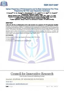
2. Amplitudes in Hilbert space Although QM allegedly is devoid of any picture of physical reality, that is not true. There are covert assumptions about physical nature embedded in the QM picture of a double slit experiment, assumptions that the waves and particles travel in the same direction, with wave interference located between the double slit barrier and the target screen (Figure–1 top).

2775 | P a g e

September 01, 2015

ISSN 2347-3487 Thomas Young made that assumption in 1800. Unfortunately, it turns out to be an illusion: a picture that exists in the minds of scientists but does not correspond to how nature works. Young was wrong, according to TEW. In nature particles follow zero energy amplitudes backwards (Figure–1 bottom). The amplitudes can be thought of as the cross section of an elementary ray. They start at every point of the target screen, penetrate backwards through the double slit barrier, and interference is located in proximity to the particle source, which we will refer to as an electron gun, even though the source could be firing Bucky balls (C60 fullerenes) instead of electrons. The probability of these elementary rays triggering a particle to follow the rays backward is proportional to the amplitude squared of the impinging rays. A particle, if triggered, follows one incident ray backwards instead of the myriad of competitors. It does so with a probability of one. It doesn’t matter which slit the electron uses. No interference that occurs subsequent to electron firing has any effect whatsoever. There is no wavefunction collapse at the target screen. Wavefunction collapse previously occurred inside the electron gun, prior to the electron being fired. A dot appears on the target screen at precisely that location from which its ray was emitted. When you write out the math (see equation 2), exactly the same interference fringe pattern is predicted on the target screen, as the one you expect (equation 1). In Figure 1–top we will use the complex number A to be the amplitude that an electron striking “X” came through slit A, and complex number B for the lower slit. The probability of an electron striking the target at any particular point, which is

 A  B 

P(x)  A  B 2  A    B   Re( AB *  A* B)  A    B    A  B  Reei(  )  ei(  ) )  A    B  2  A  B  cos(   )

(1)

Where  and  are the phases of the two complex numbers. Elementary rays leave the gun in phase and pass through slits A and B in phase but get out of phase because of the distance BX is longer than AX. One wavelength further distance translates into 2π rotations of phase. So if we move X slightly up or down the target screen so as to change the distance BX minus AX by ¼ wavelength, we will have changed the relative phase (   ) by ½ π.

Fig 1 Comparing the QM versus TEW picture of a double slit experiment Figure 1–top is a well-known picture of a double slit experiment according to QM. Figure 1–bottom shows the TEW picture of what happens: every point “X” on the target screen emanates zero energy elementary rays, which interfere in proximity to the electron gun. If an electron is fired, it follows one such ray backwards with a probability of one, and a dot appears at “X” on the target screen. In Figure 1–bottom our equation is identical. We will use the complex number A to be the amplitude that an elementary ray Æ impinging on the electron gun came through slit A, and complex number B for the amplitude that it came through slit B. The interference pattern on the target screen reflects the probability of an electron being fired in response to elementary waves from “X,” which is proportional to

2776 | P a g e

 A  B 

September 01, 2015

ISSN 2347-3487 P(x)  A  B 2  A    B   Re( AB *  A* B)  A    B    A  B  Reei(  )  ei(  ) )  A    B  2  A  B  cos(   )

(2)

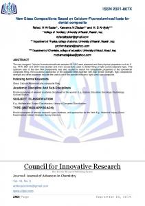
Where  and  are the phases of the two complex numbers. Elementary waves leave “X” in phase. They get out of phase because of the distance XB is longer than XA. One wavelength further distance translates into 2π rotations of phase. So if we move X slightly up or down the target screen so as to change the distance XB minus XA by ¼ wavelength, we will have changed the relative phase (   ) by ½ π. Equations 1 and 2 are identical. This shows the astonishing symmetry of QM and TEW. We will use the symbol ∏ to refer to the particle that follows an elementary ray (Æ) backwards. Every particle is attached to a ray, but not vice versa. In any volume of space there are an infinite number of elementary rays, but only a finite number of particles. We propose that at every location and in every inertial frame there are elementary rays of all frequencies and polarizations traveling at the speed of light in all directions. We are immersed in an ocean of such rays. Particles carry all the energy, momentum, spin, etc. They follow elementary rays simply because that is the way nature is rigged up. A particle must follow one ray or another. It is incapable of living without any ray. What we are describing is a cylindrical helix (see Figure 2–bottom), in which the angle of rotation, θ, is immediately involved with the length of the cylinder. Slight changes in distance translate into many rotations of the helix.

Fig 2 Elementary ray Æ (enlarged in bottom diagram) is helical in shape with amplitude A =   e

i

In Figure 2 an elementary ray Æ starts at “X”, passes through the upper slit, and impinges on the electron gun. The bottom of the diagram shows a close-up of the cylindrical helix. Figure 2 shows the model we propose for a helical elementary ray. The ray Æ has an amplitude A, which is a i

complex number, A =   e . According to this model the radius of the spiral is radius to be in Hilbert space, and we think of the Euclidean radius of a ray as zero.

r   A

We understand this

3. Hilbert and Euclidean spaces Vectors A and B can be added, as we saw in Equation 2, when the elementary ray through slit A joins the elementary ray through slit B at the electron gun. A vector can be multiplied by a scalar. Therefore these amplitudes constitute a linear i

Ği

vector space V. An adjoint of A =   e can be defined A* =   e . A helix which is left handed, like the one in Figure 2, has an adjoint that is right handed, and vice versa. The adjoints also form a linear vector space V*. For reasons discussed later, we will speak of each vector space as having n dimensions. We define an inner product

 A  B    An *)Bn .

The vector space V is complete and constitutes a Hilbert space.

n

2777 | P a g e

September 01, 2015

ISSN 2347-3487 To clarify: elementary rays, for which we use the symbol Æ, live in Euclidean space; their amplitudes live in Hilbert space. This is not the first time that a model has been proposed in QM that is an amalgam of Euclidean and Hilbert spaces. Feynman’s book QED talks about little arrows spinning around like the hand on a one handed clock. We will i

discuss this again below. Feynman’s little arrows are a simplified way of discussing A =   e . The clock faces move through Euclidean space at the speed of light, from the lamp toward the detector. Thus in Feynman’s model the tip of the hand of a clock face traces a cylindrical helix. If you take Feynman’s model and reverse the direction of the ray, so that the ray starts at the detector and travels toward the lamp, you have the model we are proposing. The two models are symmetrical. Here is the proposed mathematical description of Æ. From Figure 2 we will take X to be the real and Y to be the imaginary axis of the complex plane at the electron gun. We will take Z to be the green line that is orthogonal to the complex plane. The energy of a ray is zero:

E(® ) = 0 xÊ A cos  (t) yÊ A i sin (t)

zÊ Ğct where the radius is

rÊ |A 

angular frequency. The variable

the angle is

c

(3)

 (t)   t  2 t,

the frequency is

is the speed of light along axis Z. The frequency

the particle to which the wave can relate. The wavelength is

  2 c 

c







 (t)   , 2 t 2

and



is the

 varies depending on the energy of 2 k

,

where k is the wave number.

Although this helical object travels at the speed of light to the left on the Z axis, we are primarily interested in a cross section at the electron gun. In that plane on the gun has amplitude B

A   A  ei . Similarly, the elementary ray ÆB from “X” via slit B, impinging

  B  ei .

Since the math we are developing is tricky, we will keep things as simple as possible by limiting our discussion to a system consisting of one particle. We define  as follows:   ® +  where Æ is an elementary ray and ∏ is the particle following that ray backwards. Thus we subdivide the  of QM into a ray and particle traveling in the opposite direction. Since only the particle is visible in experiments,  appears to be located where the particle is located. Of course the ray is much longer, but, with one exception, most of it is invisible. The one exception is that nonlocal phenomena are a result of the invisible part of the elementary ray. The primary difference between  in QM and in TEW is that our wave–particle has an elementary ray embedded in it. That ray comes from the detector ahead, and may well be transporting into the wave–particle the latest information on the state of the detector toward which the wave–particle is zooming. That which QM calls “nonlocality,” TEW calls an “elementary rays.” One term is vague and nebulous. The other is specific enough for us to develop elegant mathematics and experiments to test it. Science flourishes more productively with a highly specific mathematical model than with a vague and nebulous mathematical model. We further propose that the TEW model is better for illuminating how nature is organized, whereas the QM model functions superbly for its purpose: predicting observables. We define the Dirac ket

   to be a complete set of amplitudes of the wave-particle (for observables that have    “the dynamical state of our system,” or “quantum state,” or “state vector.” For example,

discrete values), and we call a complete set of amplitudes for allowable energies, constitutes a ket which is intimately related to the Hamiltonian.

With these definitions the Schrödinger and other wave equations of QM can be imported wholesale into TEW unchanged. Even processes that are irreversible because of entropy can be imported, because entropy is a form of energy, and energy is a property of particles not waves in TEW. Particles in TEW travel in the same direction as particles in QM. Based on what has been said so far, it follows that a ket    can also be described as a vector in a linear vector space that is a Hilbert space. There is a subtle and tricky aspect to this mathematical model. We claim that behind the mathematics of Dirac notation there is another, and more basic mathematics of elementary rays. In other words, if   ® +  then    ® +  The question arises whether the particle  may be expendable from our mathematical structures. This is an open question, the answer to which is so far unknown. In other words, to what extent can we peel the outer skin off QM math (based on   ) and discover inside the math of elementary rays based on ® or

 ® ?

2778 | P a g e

September 01, 2015

ISSN 2347-3487 4. Did we make a mistake? This author keeps wondering if he made a mistake and wandered off into fanciful thinking. What reassurance do we have that the model we are developing is realistic, as opposed to being a fanciful error?

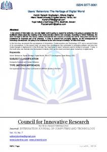
4.1 Using Feynman’s path integral model to check for errors in our model We trust Richard Feynman. In his book QED he presents the moving clock faces described above. The only difference between his model and ours is that he thought of the clocks as moving in the wrong direction through Euclidean space (see Figure 3).

Fig 3. This image is implicit, not explicit in Feynman’s book QED Feynman spoke to a lay audience that was math phobic. Instead of talking about complex vectors and linear algebra, he spoke about spinning arrows. Each arrow has an angle of rotation θ and a length. He emphasized that you have to square the length to get a probability. His imagery is that of a clock face moving through Euclidean space as shown in Figure 3. Intrinsic to Feynman’s model are all the peculiarities and problems we are discussing. He doesn’t make these problems explicit. If we take Feynman’s model (see Figure 3) and make explicit that which he didn’t say out loud, Feynman presents us a mathematics devoid of particles. Let us define Æ Backwards as being the cylindrical helices implicit in Feynman’s moving clock faces. We find internal to Feynman’s brain a covert assumption that behind the QM math based on kets   there stands a more basic math based on the cylindrical helixes of ÆBACKWARDS. Feynman apparently was comfortable with this. He didn’t see any problems in having two mathematical structures, the QM structure based on wave–particles and the underlying structure based on moving clock faces. He was a thoughtful man. He tended to see every problem from all possible angles. Hundreds of thousands of bright people have read QED and raised no objections, no red flags. So apparently there is nothing wrong with this way of thinking about quantum math. All we have done is make explicit what was implicit in Feynman’s brain. We also reversed the direction of the waves. This author feels reassured. Nevertheless, the intellectual world into which we have moved is eerie. To reiterate, we are proposing that perhaps we can peel the outer skin off QM math (based on   ) and discover inside the math of elementary rays (based on

® or  ®  ). This would be like taking the universe as science knows it, removing all the particles, and finding that the pattern and pathways that persist are somehow a ghost skeleton of pathways that stands behind or inside the reality we know. We need the particles in order to see it. Furthermore, without the particles the universe would slump into an amorphous blob. On the other hand, this peculiar way of thinking is also familiar. In any quantum experiment there are amplitudes that travel in all directions. In a double slit experiment such amplitudes penetrate both slits. Our “ghost skeleton” is simply a way of making that abstract QM idea concrete and based in physical nature independent of the observer. It was Einstein who introduced the language of ghosts, when he spoke of “spooky action at a distance.”

4.2 Divergent goals of QM versus TEW There is a conspicuous difference between our goals and the goals of Feynman (or any other branch of QM). We seek to develop a snapshot of physical nature. Intrinsic to the goal of taking a picture is that you only see one glimpse of reality with all its warts at one particular instant. Pictures ignore the thousands of different aspects of nature that are not shown in the picture. By contrast, Feynman seeks to compute a total amplitude that encompasses every possible way that nature could behave, even the remote and unlikely behaviors. That is because his goal is different than ours. His goal is to compute an “observable” that he can take to a lab to test it against experiments. Ultimately Feynman’s thinking is defined by the needs of a high energy particle lab. Our goal is defined by wanting a picture of nature independent of the observer, the way nature would work if there were no humans and no physics labs. Feynman would accuse us of making the “same mistake

2779 | P a g e

September 01, 2015

ISSN 2347-3487 that beginning physics students make,” by taking one particular Feynman diagram and believing we have a snapshot of reality. What Feynman would want us to do is to integrate across thousands of different Feynman diagrams, so as to encompass all possible ways that something would happen. Consider a photograph of a tree. For our purpose, we snap one picture that shows the tree at that particular moment. Life is always idiosyncratic and quirky, which is what makes our picture charming. However, if we wanted to compute “an observable” the way Feynman does, then we would need to integrate across all possible pictures of the tree: in each season, in daylight and starlight, in rain and drought, in forest fires and hurricanes, etc.

5. Back to Hilbert and Euclidean spaces i

Rays of multiple frequencies fit the description of having an amplitude of A   A  e at the electron gun in Figures 1 and 2. Most of them are irrelevant and should be ignored. The only ones that we will focus on have a frequency of

e 

Ee , h

where Ee is the energy of the electron about to be emitted and h is Planck’s constant. The frequency of an

elementary ray must match its particle. The wavelength of the elementary ray we seek is representation, if

 



is defined as a complete set of amplitudes for different levels of energy,

c

e



with an electron with a different energy level

r   A

In the energy

{E1, E2 , E3 , etc}, this

corresponds to a set of amplitudes for a family of coaxial elementary rays with different frequencies member of this family would have the same radius

ch . Ee

{ n 

En }. h

Every

Different members of this family would be able to connect

En  Think of a guitar string. It vibrates, sometimes in an elliptical motion, with

a multitude of different frequencies superimposed. In any specific double slit experiment, we are repeatedly dealing with electrons of the same energy is a linear combination of the basis energies. The state of our system is the

En 

That energy

    ® +      { j  E j }

where

{E j } constitute the basis energies, and  j are the amplitudes for each of those energies.

Elementary rays Æ live in Euclidean space. They carry amplitudes from Hilbert space. These elementary ray amplitudes are the analog in the physical world of the mathematical object called a probability amplitude. This is the basic reason why TEW and QM are symmetrical and are two languages for talking about the same topic: TEW being the science of the actual physical world independent of the observer; QM being the science of observables.

6. Why electrons behave differently if we look at them One of the great mysteries of the double slit experiment is complementarity: why is it that if we determine which slit an electron uses the interference fringe pattern on the target screen vanishes and vice versa? If photons are streaming through at least one of the slits, in order to determine which slit an electron went through, TEW has a simple and logical explanation, shown in Figure 4.

Fig 4 A light shines through slit A to show which slit an electron uses which destroys interference

2780 | P a g e

September 01, 2015

ISSN 2347-3487 Figure 4–top a light shining through slit A it destroys the interference of elementary rays between the double slit barrier and the electron gun. When it is turned off (Figure 4–bottom), the interference is restored. Our explanation of Figure 4 is that the light destroys the coherence of the two elementary rays (ÆA and ÆB) so they can’t interfere. If there is no interference then the electrons fired by the gun will report “no interference” at the target screen. That is in fact what is observed. We don’t know how or why the electrons disrupt the coherence of the elementary rays. Perhaps it is a change in energy. If a photon arrives at its detector with a change in energy, that might mean that it had a near encounter with an electron. The electron’s energy would reciprocally change, in the opposite direction. Therefore that electron would have to be following an elementary ray of different frequency. Thus the frequency of ÆA and ÆB would no longer match, so they would no longer interfere. Since an electron would use one slit and not both simultaneously, therefore if the frequency of ÆA would change while that of ÆB would remain the same, or vice versa. Never would both frequencies change in the same direction simultaneously. Thus the photon inadvertently destroys the coherence of the two rays. Another possibility is that the electron changes the amplitude of one of the two elementary rays, not the frequency. No matter how the electron disrupts the interference, it would produce the phenomena we observe in the lab. Problem solved!

7. Conclusion 7.1 Overview of elementary rays The doctrine of wave–particle duality is one of two major obstacles to physics students learning about elementary rays. We showed in other publications that every single experiment that allegedly “proves” wave particle duality can equally well be explained by TEW. Take the Davisson Germer experiment for example. They fired electrons at a nickel crystal and measured the voltage and angle at which the electrons ricocheted. Their data showed an unexpected spur at o 50 for electrons fired at 54 volts, which meant there were waves of 1.67 Å refracting through the crystal and interacting with electron particles. This was taken as absolute “proof” of wave particle duality, and Davisson was given a Nobel Prize. But no one has ever demonstrated whether those waves travel in the same direction as the electrons, or the opposite direction. From other experiments it is clear that waves and particles travel in opposite directions. Once we open our minds to the idea that particles follow elementary ray amplitudes backwards, it becomes urgent to understand what these rays look like and how they function. Quantum mathematics is our guide, our roadmap. Based on the ubiquity of amplitudes in quantum math, and the ubiquity of rays in TEW, we propose our corkscrew model. We know from quantum math that these corkscrews are very orderly and predictable. They support the Dirac notation and a vast superstructure of linear algebra. It is also clear that interference is delicate, to the point that if you look at it cross-eyed it vanishes. In the double slit experiments QM calls this phenomenon “complementarity.” QM however offers no plausible explanation for the doctrine of complementarity. Feynman was fond of saying that electrons don’t like to be looked at, and behave differently if we watch them. We have provided a simple and logical explanation of that phenomenon. Apparently electrons act different when we watch them because watching them destroys the coherence of one elementary ray with its twin. This means that coherence is fragile. We can learn a lot about coherence from the large body of experiments on double slit experiments in which every single effort, no matter how ingenious, to learn which slit an electron uses, destroys the interference fringe pattern on the target screen. There is an entire science of elementary rays waiting for young physicists to explore. There is however a second major obstacle to this happening: young physicists never heard of TEW. Why? This is not from lack of effort on our part. Leading journals of physics routinely reject articles we submit, saying things like “This article has no scientific merit.” When this author electronically submitted an article to the leading journal Science, it was rejected in less than fifteen minutes with the comment, “Not the kind of thing we publish.” So why is there such a roadblock to learning about a new idea? This is easy to understand once you comprehend the history of TEW, and the history of paradigm shifts.

7.2 The history of TEW and of paradigm shifts TEW did not arise from incremental advances in mainstream physics. Lewis E. Little, after getting his PhD in physics, wanted to find a local and realistic explanation of quantum experiments. He cooked up TEW over the course of several decades, working alone weekends and nights in his kitchen, talking to no one. Eventually he cracked the code. He thought of waves travelling in the opposite direction as particles. Such a bizarre idea had never occurred to anyone before. This led to TEW, which not only eliminates nonlocality, but, as we showed in other publications, provides a local and realistic explanation of Bell test experiments. He first published his idea in 1996, expecting the physics community would applaud. Instead his ideas were ignored. For many years this author worked with Little (see photo at the end of this article) seeking to promote his theory within the physics community. There were scholarly presentations at the American Physical Society and articles in physics research journals, as well as videos on YouTube (elwavetheory) and we plan to develop a Facebook page. This author was the first to publish an explanation of the Bell test experiments based on bi–rays from TEW. TEW is a newborn science: many issues need to be worked out. The one that gets under my skin is how the math of

2781 | P a g e

September 01, 2015

ISSN 2347-3487 QM relates to the math of TEW. I’m trained in mathematics. It took me years to figure out. I lost sleep and obsessed about a mathematical crosswalk between QM and TEW. The pivotal step was an image of corkscrews that crystallized in my brain while I was reading Feynman’s book QED. Feynman invokes images of spinning arrows like a hand on a clock: a hand (arrow) represents an amplitude. Meanwhile the clock faces move through Euclidean space, so the tip of the arrow traces a cylindrical helix, at least in my imagination. Thomas Kuhn observes seismic paradigm shifts of the past were despised in their time [13]. From the viewpoint of the establishment, a new paradigm threatens the status quo and make no sense at all.[xx] Consider plate tectonics. Alfred Wegener proposed his continental drift theory in 1912.[14] All continents used to be part of a supercontinent for which he coined the name Pangaea. After Pangaea broke up, the continents drifted apart. He had no idea why or how. Scientists were extremely hostile to this idea. A leading geologist, Sir Harold Jeffrey thought it was preposterous. The American Association of Petroleum Geologists officially said that Wegener’s idea made no sense at all. Rollin Chamberlin wrote, "Wegener's hypothesis in general is of the footloose type, in that it is less bound by restrictions or tied down by awkward, ugly facts than most." Geologist Barry Willis said, “further discussion of it merely encumbers the literature and befogs the mind of students.” Geologist Thomas Chamberlain, wrote, "If we are to believe in Wegener's hypothesis we must forget everything which has been learned in the past 70 years and start all over again." Even within Wegener’s family, his fatherin-law, a leading meteorologist, publically criticized Wegener’s idea as stupid. After Wegener’s death in 1930 his idea was swept under the rug and forgotten. When I was a child in the 1940’s we thought that the ocean floor consisted of thousands of miles of flat sand. If continents moved we couldn’t understand how they would plow through the sand. In the 1950’s Navy sonar discovered a mid-oceanic mountain range. Studies of magnetism of rocks suggested mid-ocean spreading in the 1960s. As more was learned about the ocean floor, scientists slowly and cautiously ventured to support the continental drift theory. After one century Wegener’s obscure crackpot idea, now called “plate tectonics,” is taken for granted by all geologists!

8. Acknowledgments Lewis E. Little taught me the basics of TEW.

9. Bibliography [1] J. J. Binney and D. Skinner, The Physics of Quantum Mechanics, c2010, available online at http://wwwthphys.physics.ox.ac.uk/people/JamesBinney/qb.pdf, access date May 20, 2015 [2]

R. P. Feynman, QED (Oxford University Press and Princeton U. Press, 1985).

[3] J. H. Boyd, A paradigm shift in mathematical physics, Part 1: the Theory of Elementary Waves (TEW), Journal of Advances in Mathematics, 11, #3, (July 2015). [4] J. H. Boyd, A paradigm shift in mathematical physics, Part 2: A new local realism explains Bell test & other experiments, Journal of Advances in Mathematics, 11, #4, (July 2015). [5] J. H. Boyd, A paradigm shift in mathematical physics, Part 3: A mirror image of Feynman’s quantum electrodynamics (QED), Journal of Advances in Mathematics (in press). [6] J. H. Boyd, A new variety of local realism explains a Bell test experiment: the Theory of Elementary Waves (TEW) with no hidden variables, Journal of Advances in Physics 8, 2051-58 (Mar 2015). [7] J. H. Boyd, The Theory of Elementary Waves eliminates Wave Particle Duality, Journal of Advances in Physics 7, 1916-1922 (Feb 2015). [8] J. H. Boyd, Re-thinking Alain Aspect's 1982 Bell test experiment with delayed choice, Physics Essays 26 (4) 582591 (2013). [9] J. H. Boyd, Re-thinking a delayed choice quantum eraser experiment: a simple baseball model, Physics Essays 26, 100-109 (March 2013), (doi: 10.4006/0836-1398-26.1.100). [10] J. H. Boyd, Rethinking a Wheeler delayed choice gedanken experiment, Physics Essays 25, (3) pp. 390-396, 2012. doi: http://dx.doi.org/10.4006/0836-1398-25.3.390 [11]

L. E. Little, Theory of Elementary Waves, Physics Essays 9 (1), 100-134 (1996).

[12]

L. E. Little, Theory of Elementary Waves, (New Classics Library, New York, 2009).

[13]

T. S. Kuhn, The Structure of Scientific Revolutions, (Chicago: U. of Chicago Press, 1996).

[14]

A. Wegener, Die Entstehung der Kontinente, Petermanns Geogr. Mitt. 7, 185 - 308, (1912).

Author’s biography with Photo Dr. Boyd was born in 1943 in northern New Jersey, USA, the son of a factory worker family in which no one had ever been to college. In high school he helped his father dig a basement by hand, using a pick, shovel and wheelbarrow. As a teenager he and his cousin, Lewis E. Little, played three dimensional tic-tac-toe, and developed strategies for four dimensional tic-tac-toe. Boyd chose which college to apply to based on Little’s advice about which had the best Applied Math department. Boyd’s undergraduate degree in mathematics was from Brown University in 1965, three years after

2782 | P a g e

September 01, 2015

ISSN 2347-3487 Little graduated from Brown in physics. Following Dr. Martin Luther King in the Civil Rights movement, Boyd was in Mississippi in 1965, where he learned that being denounced as an outside agitator did not mean one was doing the wrong thing. Boyd has post-graduate degrees from Harvard, Yale and Case Western Reserve Universities, has served on the research faculty of the National Institutes of Health for seven years, and has been on the faculty of the Yale Medical School. His day job is as a physician: a psychiatrist. Boyd retired after a quarter century at Waterbury Hospital, Waterbury CT, a Yale teaching hospital at which he served as chairman of behavioral health and chairman of ethics. Fifty five years ago Boyd abandoned his first love (mathematics) because of his belief that no mathematician over the age of 25 ever discovered anything important, and he was rapidly approaching that age. He wanted to be in a field where age and experience counted for you, not against you. A rewarding career in medicine followed. Then Andrew Wiles proved Femat’s last theorem at age forty and Lewis Little discovered elementary waves at age fifty-two. With this series of articles in JAP the author discovered, to his astonishment, that even this old dog can learn some new tricks. Boyd has published in the New England Journal of Medicine, Journal of Advances in Physics, Journal of Advances in Mathematics and Physics Essays. Boyd is currently working on videos to present his ideas via YouTube. See for example: https://www.youtube.com/watch?v=cmM8Dr3Hbb0&feature=youtu.be

Lewis E. Little

2783 | P a g e

Jeffrey H. Boyd

September 01, 2015