Counterexample Guided Inductive Optimization

Counterexample Guided Inductive Optimization Rodrigo F. Araújoa , Higo F. Albuquerqueb , Iury V. de Bessab , Lucas C. Cordeiroc , João Edgar C. Filhob

arXiv:1704.03738v1 [cs.AI] 11 Apr 2017

a Federal

Institute of Amazonas, Campus Manaus Distrito Industrial, Avenida Governador Danilo Areosa, 1672, Distrito Industrial, 69075351, Manaus, AM, Brasil b Department of Electricity, Federal University of Amazonas, Avenida General Rodrigo Octávio, 6200, Coroado I, Manaus, AM, 69077-000 c Department of Computer Science, University of Oxford, Wolfson Building, Parks Road, OXFORD, OX1 3QD, UK

Abstract This paper describes three variants of a counterexample guided inductive optimization (CEGIO) approach based on Satisfiability Modulo Theories (SMT) solvers. In particular, CEGIO relies on iterative executions to constrain a verification procedure, in order to perform inductive generalization, based on counterexamples extracted from SMT solvers. CEGIO is able to successfully optimize a wide range of functions, including non-linear and non-convex optimization problems based on SMT solvers, in which data provided by counterexamples are employed to guide the verification engine, thus reducing the optimization domain. The present algorithms are evaluated using a large set of benchmarks typically employed for evaluating optimization techniques. Experimental results show the efficiency and effectiveness of the proposed algorithms, which find the optimal solution in all evaluated benchmarks, while traditional techniques are usually trapped by local minima. Keywords: Satisfiability Modulo Theories (SMT), Model checking, Global optimization, Non-convex optimization

1. Introduction Optimization is an important research topic in many fields, especially in computer science and engineering [1]. Commonly, scientists and engineers have to find parameters, which optimize the behavior of a given system or the value of a given function (i.e., an optimal solution). Optimization characterizes and distinguishes the engineering gaze over a problem; for this particular reason, previous studies showed that optimization is one of the main differences between engineering design and technological design [2]. Computer science and optimization maintain a symbiotic relationship. Many important advances of computer science are based on optimization theory. As example, planning and decidability problems (e.g., game theory [3]), resource allocation problems (e.g., hardware/software co-design [4]), and computational estimation and approximation (e.g., numerical analysis [5]) represent April 13, 2017

important optimization applications. Conversely, computer science plays an important role in recent optimization studies, developing efficient algorithms and providing respective tools for supporting model management and results analysis [6]. There are many optimization techniques described in the literature (e.g., simplex [7], gradient descent [8], and genetic algorithms [9]), which are suitable for different classes of optimization problems (e.g., linear or non-linear, continuous or discrete, convex or non-convex, and single- or multi-objective). These techniques are usually split into two main groups: deterministic and stochastic optimization. Deterministic optimization is the classic approach for optimization algorithms, which is based on calculus and algebra operators, e.g., gradients and Hessians [10]. Stochastic optimization employs randomness in the optima search procedure [10]. This paper presents a novel class of search-based optimization algorithm that employs non-deterministic representation of decision variables and constrains the state-space search based on counterexamples produced by an SMT solver, in order to ensure the complete global optimization without employing randomness. This class of techniques is defined here as counterexample guided inductive optimization (CEGIO), which is inspired by the syntax-guided synthesis (SyGuS) to perform inductive generalization based on counterexamples provided by a verification oracle [11]. Particularly, a continuous non-convex optimization problem is one of the most complex problems. As a result, several traditional methods (e.g., NewtonRaphson [1] and Gradient Descent [8]) are inefficient to solve that specific class of problems [1]. Various heuristics are developed for obtaining approximated solutions to those problems; heuristics methods (e.g., ant colony [12] and genetic algorithms [9]) offer faster solutions for complex problems, but they sacrifice the system’s correctness and are easily trapped by local optimal solutions. This paper presents a novel counterexample guided inductive optimization technique based on SMT solvers, which is suitable for a wide variety of functions, even for non-linear and non-convex functions, since most realworld optimization problems are non-convex. The function evaluation and the search for the optimal solution is performed by means of an iterative execution of successive verifications based on counterexamples extracted from SMT solvers. The counterexample provides new domain boundaries and new optima candidates. In contrast to other heuristic methods (e.g., genetic algorithms), which are usually employed for optimizing this class of function, the present approaches always find the global optimal point. This study extends the previous work of Araújo et al. [13] and presents three variants of a counterexample guided inductive optimization approach based on SMT solvers, which improve the technique performance for specific class of functions. Furthermore, the experimental evaluation is largely expanded, since the algorithms are executed for additional optimization problems and the performance of each proposed algorithm is compared to six well-known optimization techniques. The present CEGIO approaches are able to find the correct global minima for 100% of the benchmarks, while other techniques are usually trapped by local minima, thus leading to incorrect so-

2

lutions. 1.1. Contributions Our main original contributions are: • Novel counterexample guided inductive optimization approach. This work describes three novel variants of a counterexample guided inductive optimization approach based on SMT solvers: generalized, simplified, and fast algorithms. The generalized algorithm can be used for any constrained optimization problem and presents minor improvements w.r.t. Araújo et al. [13]. The simplified algorithm is faster than the generalized one and can be employed if information about the minima location is provided, e.g., the cost function is semi-definite positive. The fast algorithm presents a significant speed-up if compared to the generalized and simplified ones, but it can only be employed for convex functions. • Convergence Proofs. This paper presents proofs of convergence and completeness (omitted in Araújo et al. [13]) for the proposed counterexample guided inductive optimization algorithms. • SMT solvers performance comparison. The experiments are performed with three different SMT solvers: Z3 [14], Boolector [15], and MathSAT [16]. The experimental results show that the solver choice can heavily influence the method performance. • Additional benchmarks. The benchmark suite is expanded to 30 optimization functions extracted from the literature [17]. • Comparison with existing techniques. The proposed technique is compared to genetic algorithm [9], particle swarm [18], pattern search [19], simulated annealing [20], and nonlinear programming [21], which are traditional optimization techniques employed for non-convex functions. 1.2. Availability of Data and Tools Our experiments are based on a set of publicly available benchmarks. All tools, benchmarks, and results of our evaluation are available on a supplementary web page http://esbmc.org/benchmarks/jscp2017.zip. 1.3. Outline Section 2 discusses related studies. Section 3 provides an overview of optimization problems and techniques, and describes background on software model checking. Section 4 describes the ANSI-C model developed for optimization problems that is suitable for the counterexample guided inductive optimization procedure. Section 5 describes the generalized and simplified optimization algorithms and respective completeness proofs. Section 6 describes the fast optimization algorithm and respective completeness proof. Section 7 reports the experimental results for evaluating all proposed optimization algorithms, while Section 8 concludes this work and proposes further studies.

3

2. Related Work SMT solvers have been widely applied to solve several types of verification, synthesis, and optimization problems. They are typically used to check the satisfiability of a logical formula, returning assignments to variables that evaluate the formula to true, if it is satisfiable; otherwise, the formula is said to be unsatisfiable. Nieuwenhuis and Oliveras [22] presented the first research about the application of SMT to solve optimization problems. Since then, SMT solvers have been used to solve different optimization problems, e.g., minimize errors in linear fixed-point arithmetic computations in embedded control software [23]; reduce the number of gates in FPGA digital circuits [24]; hardware/software partition in embedded systems to decide the most efficient system implementation [25–27]; and schedule applications for a multi-processor platform [28]. All those previous studies use SMT-based optimization over a Boolean domain to find the best system configuration given a set of metrics. In particular, in Cotton et al. [28] the problem is formulated as a multi-objective optimization problem. Recently, Shoukry et al. [29] proposed a scalable solution for synthesizing a digital controller and motion planning for under-actuated robots from LTL specifications. Such solution is more flexible and allows solving a wider variety of problems, but they are focused on optimization problems that can be split into a Boolean part and other convex part. In addition, there were advances in the development of different specialized SMT solvers that employ generic optimization techniques to accelerate SMT solving, e.g., the ABsolver [30], which is used for automatic analysis and verification of hybrid-system and control-system. The ABsolver uses a non-linear optimization tool for Boolean and polynomial arithmetic and a lazy SMT procedure to perform a faster satisfiability checking. Similarly, CalCs [31] is also an SMT solver that combines convex optimization and lazy SMT to determine the satisfiability of conjunctions of convex non-linear constraints. Recently, Shoukry et al. [32] show that a particular class of logic formulas (named SMC formulas) generalizes a wide range of formulas over Boolean and nonlinear real arithmetic, and propose the Satisfiability Modulo Convex Optimization to solve satisfiability problems over SMC formulas. Our work differs from those previous studies [30–32] since it does not focus on speeding up SMT solvers, but it employs an SMT-based model-checking tool to guide (via counterexample) an optimization search procedure in order to ensure the global optimization. Recently, νZ [33] extends the SMT solver Z3 for linear optimization problems; Li et al. proposed the SYMBA algorithm [34], which is an SMT-based symbolic optimization algorithm that uses the theory of linear real arithmetic and SMT solver as black box. Sebastiani and Trentin [35] present OptiMathSat, which is an optimization tool that extends MathSAT5 SMT solver to allow solving linear functions in the Boolean, rational, and integer domains or a combination of them; in Sebastiani and Tomasi [36], the authors used a combination of SMT and LP techniques to minimize rational functions; the related work [37] extends their work with linear arithmetic on the mixed integer/rational domain, thus combining SMT, LP, and ILP techniques. 4

As an application example, Pavlinovic et al. [38] propose an approach which considers all possible compiler error sources for statically typed functional programming languages and reports the most useful one subject to some usefulness criterion. The authors formulate this approach as an optimization problem related to SMT and use νZ to compute an optimal error source in a given ill-typed program. The approach described by Pavlinovic et al., which uses MaxSMT solver νZ, shows a significant performance improvement if compared to previous SMT encodings and localization algorithms. Most previous studies related to SMT-based optimization can only solve linear problems over integer, rational, and Boolean domains in specific cases, leading to limitations in practical engineering applications. Only a few studies [29] are able to solve non-linear problems, but they are also constrained to convex functions. In contrast, this paper proposes a novel counterexample guided inductive optimization method based on SMT solvers to minimize functions, linear or non-linear, convex or non-convex, continuous or discontinuous. As a result, the proposed methods are able to solve optimization problems directly on the rational domain with adjustable precision, without using any other technique to assist the state-space search. Furthermore, our proposed methods employ a model-checking tool to generate automatically SMT formulas from an ANSI-C model of the optimization problem, which makes the representation of problems for SMT solving easy for engineers. 3. Preliminaries 3.1. Optimization Problems Overview Let f : X → R be a cost function, such that X ⊂ R n represents the decision variables vector x1 , x2 , ..., xn and f ( x1 , x2 , ..., xn ) ≡ f (x). Let Ω ⊂ X be a subset settled by a set of constraints. Definition 1. A multi-variable optimization problem consists in finding an optimal vector x, which minimizes f in Ω. According to Definition 1, an optimization problem can be written as min s.t.

f (x), x ∈ Ω.

(1)

In particular, this optimization problem can be classified in different ways w.r.t. constraints, decision variables domain, and nature of cost function f . All optimization problems considered here are constrained, i.e., decision variables are constrained by the subset Ω. The optimization problem domain X that contains Ω can be the set of N, Z, Q, or R. Depending on the domain and constraints, the optimization search-space can be small or large, which influences the optimization algorithms performance. The cost function can be classified as linear or non-linear; continuous, discontinuous or discrete; convex or non-convex. Depending on the cost function nature, the optimization problem can be hard to solve, given the time and memory resources [39]. Particularly, non-convex optimization problems are the most difficult ones w.r.t. the cost function nature. A non-convex cost 5

function is a function whose epigraph is a non-convex set and consequently presents various inflexion points that can trap the optimization algorithm to a sub-optimal solution. A non-convex problem is necessarily a non-linear problem and it can also be discontinuous. Depending on that classification, some optimization techniques are unable to solve the optimization problem, and some algorithms usually point to suboptimal solutions, i.e., a solution that is not a global minimum of f , but it only locally minimizes f . Global optimal solutions of the function f , aforementioned, can be defined as Definition 2. A vector x∗ ∈ Ω is a global optimal solution of f in Ω iff f (x∗ ) ≤ f ( x ), ∀x ∈ Ω. 3.2. Optimization Techniques Different optimization problems offer different difficulties to their particular solutions. Such complexity is mainly related to the ruggedness (e.g., continuity, differentiability, and smoothness) and dimensionality of the problem (i.e., the dimension, and for the finite case, the number of elements of Ω). Depending on these factors, different optimization techniques can be more efficient to solve a particular optimization problem. Generally, traditional optimization techniques can be divided into two groups: deterministic and stochastic optimization. The deterministic techniques employ a search engine, where each step is directly and deterministically related to the previous steps [40]. In summary, deterministic techniques can be gradient-based or enumerative search-based. Gradient-based techniques search for points, where the gradient of cost function is null (∇ f (x) = 0), e.g., gradient-descent [41] and Newton’s optimization [1]. Although they are fast and efficient, those techniques are unable to solve non-convex or non-differentiable problems. Enumerative search-based optimization consists in scanning the search-space by enumerating all possible points and comparing cost function with best previous values, e.g., dynamic programming, branch and bound [42], and pattern search [43]. Stochastic techniques employ randomness to avoid the local minima and to ensure the global optimization; such techniques are usually based on metaheuristics [44]. This class of techniques has become very popular in the last decades and has been used in all types of optimization problems. Among those stochastic techniques, simulated annealing [20], particle swarm [18], and evolutionary algorithms (e.g., genetic algorithms [9]) are usually employed in practice. Recently, optimization techniques and tools that employ SMT solvers and non-deterministic variables were applied to solve optimization problems [29– 31, 33–37, 45], which searches for the global optima in a search-space that is symbolically defined and uses counterexamples produced by SMT solvers to further constrain the search-space. The global optima is the set of values for the decision variables that makes an optimization proposition satisfiable. The technique presented here is the first optimization method based on SMT solvers and inductive generalization described in the literature, which is able to solve non-convex problems over R.

6

3.3. Model Checking Model checking is an automated verification procedure to exhaustively check all (reachable) system’s states [46]. The model checking procedure typically consists of three steps: modeling, specification, and verification. Modeling is the first step, where it converts the system to a formalism that is accepted by a verifier. The modeling step usually requires the use of an abstraction to eliminate irrelevant (or less) important system details [47]. The second step is the specification, which describes the system’s behavior and the property to be checked. An important issue in the specification is the correctness. Model checking provides ways to check whether a given specification satisfies a system’s property, but it is difficult to determine whether such specification covers all properties in which the system should satisfy. Finally, the verification step checks whether a given property is satisfied w.r.t. a given model, i.e., all relevant system states are checked to search for any state that violates the verified property. In case of a property violation, the verifier reports the system’s execution trace (counterexample), which contains all steps from the (initial) state to the (bad) state that lead to the property violation. Errors could also occur due to incorrect system modeling or inadequate specification, thus generating false verification results. 3.3.1. Bounded Model Checking (BMC) BMC is an important verification technique, which has presented attractive results over the last years [48]. BMC techniques based on Boolean Satisfiability (SAT) [49] or Satisfiability Modulo Theories (SMT) [50] have been successfully applied to verify single- and multi-threaded programs, and also to find subtle bugs in real programs [51, 52]. BMC checks the negation of a given property at a given depth over a transition system M. Definition 3. [49] – Given a transition system M, a property φ, and a bound k; BMC unrolls the system k times and translates it into a verification condition (VC) ψ, which is satisfiable iff φ has a counterexample of depth less than or equal to k. In this study, the ESBMC tool [53] is used as verification engine, as it represents one of the most efficient BMC tools that participated in the last software verification competitions [48]. ESBMC finds property violations such as pointer safety, array bounds, atomicity, overflows, deadlocks, data race, and memory leaks in single- and multi-threaded C/C++ software. It also verifies programs that make use of bit-level, pointers, structures, unions, fixed- and floating-point arithmetic. Inside ESBMC, the associated problem is formulated by constructing the following logical formula ψk = I (S0 ) ∧

k i^ −1 _

γ ( s j , s j +1 ) ∧ φ ( s1 )

(2)

i =0 j =0

where φ is a property and S0 is a set of initial states of M, and γ(s j , s j+1 ) is the transition relation of M between time steps j and j + 1. Hence, I (S0 ) ∧ V i −1 j =0 γ ( s j , s j +1 ) represents the executions of a transition system M of length i. The above VC ψ can be satisfied if and only if, for some i ≤ k there exists 7

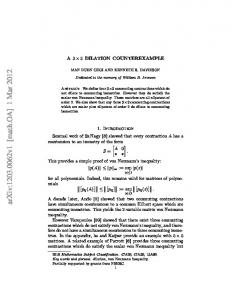
a reachable state at time step i in which φ is violated. If the logical formula (2) is satisfiable (i.e., returns true), then the SMT solver provides a satisfying assignment (counterexample). Definition 4. A counterexample for a property φ is a sequence of states s0 , s1 , . . . , sk with s0 ∈ S0 , sk ∈ Sk , and γ (si , si+1 ) for 0 ≤ i < k that makes (2) satisfiable. If it is unsatisfiable (i.e., returns false), then one can conclude that there is no error state in k steps or less. In addition to software verification, ESBMC has been applied to ensure correctness of digital filters and controllers [54–56]. Recently, ESBMC has been applied to optimize HW/SW co-design [25–27]. 4. Verification Model for Counterexample Guided Inductive Optimization 4.1. Modeling Optimization Problems using a Software Model Checker There are two important directives in the C/C++ programming language, which can be used for modeling and controlling a verification process: ASSUME and ASSERT. The ASSUME directive can define constraints over (non-deterministic) variables, and the ASSERT directive is used to check system’s correctness w.r.t. a given property. Using these two statements, any off-the-shelf C/C++ model checker (e.g., CBMC [52], CPAChecker [57], and ESBMC [53]) can be applied to check specific constraints in optimization problems, as described by Eq. (1). Here, the verification process is iteratively repeated to solve an optimization problem using intrinsic functions available in ESBMC (e.g., __ESBMC_assume and __ESBMC_assert). We apply incremental BMC to efficiently prune the state-space search based on counterexamples produced by an SMT solver. Note that completeness is not an issue here (cf. Definitions 1 and 2) since our optimization problems are represented by loop-free programs [58]. 4.2. Illustrative Example The Ursem03’s function is employed to illustrate the present SMT-based optimization method for non-convex optimization problems [17]. The Ursem03’s function is represented by a two-variables function with only one global minimum in f ( x1 , x2 ) = −3, and has four regularly spaced local minima positioned in a circumference, with the global minimum in the center. Ursem03’s function is defined by Eq. (3); Fig. 1 shows its respective graphic.   π  (2 − | x2 |)(3 − | x2 |) π  (2 − | x1 |)(3 − | x1 |) − sin 2.2πx2 − (3) f ( x1 , x2 ) = − sin 2.2πx1 − 2 4 2 4

4.3. Modeling The modeling process defines constraints, i.e., Ω boundaries (cf. Section 3.1). This step is important for reducing the state-space search and consequently for avoiding the state-space explosion by the underlying model-checking procedure. Our verification engine is not efficient for unconstrained optimization;

8

Figure 1: Ursem03’s function

fortunately, the verification time can be drastically reduced by means of a suitable constraint choice. Consider the optimization problem given by Eq. (4), which is related to the Ursem03’s function given in Eq. (3): min s.t.

f ( x1 , x2 ) x1 ≥ 0 x2 ≥ 0.

(4)

Note that inequalities x1 ≥ 0 and x2 ≥ 0 are pruning the state-space search to the first quadrant; however, even so it produces a (huge) state-space to be explored since x1 and x2 can assume values with very high modules. The optimization problem given by Eq. (4) can be properly rewritten as Eq. (5) by introducing new constraints. The boundaries are chosen based on Jamil and Yang [17], which define the domain in which the optimization algorithms can evaluate the benchmark functions. min s.t.

f ( x1 , x2 ) −2 ≤ x 1 ≤ 2 −2 ≤ x2 ≤ 2.

(5)

From the optimization problem definition given by Eq. (5), the modeling step can be encoded, where decision variables are declared as non-deterministic variables constrained by the ASSUME directive. In this case, −2 ≤ x1 ≤ 2 and −2 ≤ x2 ≤ 2. Fig. 2 shows the respective C code for modeling Eq. (5). Note that in Figure 2, the decision variables x1 and x2 are declared as floatingpoint numbers initialized with non-deterministic values; we then constraint the state-space search using assume statements. The objective function of Ursem‘s function is then declared as described by Eq. 3. 9

1 2 3 4 5 6 7 8 9 10 11 12 13 14 15

# include " math2 . h " fl o at nondet_float ( ) ; i n t main ( ) { // define decision variables f l o a t x1 = n o n d e t _ f l o a t ( ) ; f l o a t x2 = n o n d e t _ f l o a t ( ) ; / / c o n s t r a i n t h e s t a t e −s p a c e s e a r c h __ESBMC_assume ( ( x1 >= − 3) && ( x1 < = 3 ) ) ; __ESBMC_assume ( ( x2 >= − 2) && ( x2 < = 2 ) ) ; / / c o m p u t i n g Ursem ’ s f u n c t i o n float fobj ; f o b j = − s i n ( 2 . 2 ∗ p i ∗x1−p i /2)∗(2 − abs ( x1 ))(3 − abs ( x1 ) ) / 4 − s i n ( 2 . 2 ∗ p i ∗x2−p i /2)∗(2 − abs ( x2 ))(3 − abs ( x2 ) ) / 4 ; return 0 ; } Figure 2: C Code for the optimization problem given by Eq. (5).

4.4. Specification The next step of the proposed methodology is the specification, where the system behavior and the property to be checked are described. For the Ursem03’s function, the result of the specification step is the C program shown in Fig. 3, which is iteratively checked by the underlying verifier. Note that the decision variables are declared as integer type and their initialization depends on a given precision p, which is iteratively adjusted once the counterexample is produced by the SMT solver. Indeed, the C program shown in Fig. 2 leads the verifier to produce a considerably large state-space exploration, if the decision variables are declared as non-deterministic floating-point type. In this study, decision variables are defined as non-deterministic integers, thus discretizing and reducing the state-space exploration; however, this also reduces the optimization process precision. To trade-off both precision and verification time, and also to maintain convergence to an optimal solution, the underlying model-checking procedure has to be iteratively invoked, in order to increase its precision for each successive execution. An integer variable p = 10n is created and iteratively adjusted, such that n is the amount of decimal places related to the decision variables. Additionally, a new constraint is inserted; in particular, the new value of the objective function f (x( i) ) at the i-th must not be greater than the value obtained in the previous iteration f (x( i−1)). Initially, all elements in the statespace search Ω are candidates for optimal points, and this constraint cutoffs several candidates on each iteration. In addition, a property has to be specified to ensure convergence to the minimum point on each iteration. This property specification is stated by means of an assertion, which checks whether the literal loptimal given in Eq. (6) is satisfiable for every optimal candidate f c remaining in the state-space search (i.e., traversed from lowest to highest). loptimal ⇐⇒ f (x) > f c 10

(6)

The verification procedure stops when the literal loptimal is not satisfiable, i.e., if there is any x( i) for which f (x( i) ) ≤ f c ; a counterexample shows such xi , approaching iteratively f (x) from the optimal x∗ . Fig. 3 shows the initial specification for the optimization problem given by Eq. (5). The initial value of the objective function can be randomly initialized. For the example in Fig. 3, f (x(0) ) is arbitrarily initialized to 100, but the present optimization algorithm works for any initial state. 1 2 3 4 5 6 7 8 9 10 11 12 13 14 15 16 17 18 19 20 21 22 23 24 25 26

# include " math2 . h " # define p 1 / / p r e c i s i o n v a r i a b l e i n t nondet_int ( ) ; fl o at nondet_float ( ) ; i n t main ( ) { float f_ i = 100; / / previous o b j e c t i v e function value i n t l i m _ i n f _ x 1 = −2∗p ; i n t lim_sup_x1 = 2∗p ; i n t l i m _ i n f _ x 2 = −2∗p ; i n t lim_sup_x2 = 2∗p ; i n t X1 = n o n d e t _ i n t ( ) ; i n t X2 = n o n d e t _ i n t ( ) ; f l o a t x1 = f l o a t n o n d e t _ f l o a t ( ) ; f l o a t x2 = f l o a t n o n d e t _ f l o a t ( ) ; __ESBMC_assume ( ( X1>= l i m _ i n f _ x 1 ) && ( X1= l i m _ i n f _ x 2 ) && ( X2f _i __ESBMC_assume ( f o b j < f _ i ) ; assert ( fobj > f_i ) ; return 0 ; } Figure 3: C code after the specification of Eq. (5).

4.5. Verification Finally, in the verification step, the C program shown in Fig. 3 is checked by the verifier and a counterexample is returned with a set of decision variables x, for which the objective function value converges to the optimal value. A specified C program only returns a successful verification result if the previous function value is the optimal point for that specific precision (defined by p), i.e., f (x( i−1)) = f (x∗ ). For the example shown in Fig. 3, the verifier shows a counterexample with the following decision variables: x1 = 2 and x2 = 0. These decision variable are used to compute a new minimum candidate, note that f (2, 0) = −1.5, which is the new minimum candidate solution provided by this verification step. Naturally, it is less than the initial value (100), and 11

this verification can be repeated with the new value of f (x( i−1) ), in order to obtain an objective function value that is close to the optimal point on each iteration. Note that the data provided by the counterexample is crucial for the algorithm convergence and for the state-space search reduction. 5. Counterexample Guided Inductive Optimization of Non-convex Functions This section presents two variants of the Counterexample Guided Inductive Optimization (CEGIO) algorithm for global constrained optimization. A generalized CEGIO algorithm is explained in Subsection 5.1, together with a convergence proof in Subsection 5.2, while Subsection 5.3 presents a simplified version of that algorithm. 5.1. CEGIO: the Generalized Algorithm (CEGIO-G) The generalized SMT-based optimization algorithm previously presented by Araújo et al. [13] is able to find the global optima for any optimization problem that can be modeled with the methodology presented in Section 4. The execution time of that algorithm depends on how the state-space search is restricted and on the number of the solution decimal places. Specifically, the algorithm presents a fixed-point solution with adjustable precision, i.e., the number of decimal places can be defined. Naturally, for integer optimal points, this algorithm returns the correct solution quickly. However, this algorithm might take longer for achieving the optimal solution of unconstrained optimization problems with non-integer solutions since it depends on the required precision. Although this algorithm frequently produces a longer execution time than other traditional techniques, its error rate is typically lower than other existing methods, once it is based on a complete and sound verification procedure. Alg. 1 shows an improved version of the algorithm presented by Araújo et al. [13]; this algorithm is denoted here as ”Generalized CEGIO algorithm” (CEGIO-G). Alg. 1 repeats the specification and verification steps, described in Section 4, until the optimal solution x∗ is found. The precision of optimal solution defines the desired precision variable ǫ. An unitary value of ǫ results in integer solutions. Solution with one decimal place is obtained for ǫ = 10, two decimal places are achieved for ǫ = 100, i.e., the number of decimal places η for the solution is calculated by means of the equation η = log ǫ.

(7)

After the variable initialization and declaration (lines 1-3 of Alg. 1), the search domain Ω is specified in line 5, which is defined by lower and upper bounds of the x variable, and in line 6, the model for function, f ( x ), is defined. The specification step (line 8) is executed for each iteration until the desired precision is achieved. In this specific step, the search-space is remodelled for the i-th precision and it employs previous results of the optimization process, i.e., f (x( i−1) ). The verification step is performed in lines 9-10, where the candidate function f c , i.e., f (x( i−1)) is analyzed by means of the satisfiability check 12

input : A cost function f (x), the space for constraint set Ω, and a desired precision ǫ output : The optimal decision variable vector x∗ , and the optimal value of function f (x∗ ) 1 2 3 4 5 6 7 8 9 10 11 12 13 14 15 16

Initialize f (x(0) ) randomly and i = 1 Initialize the precision variable with p = 1 Declare the auxiliary variables x as non-deterministic integer variables while p ≤ ǫ do Define bounds for x with the ASSUME directive, such that x ∈ Ωη Describe a model for f (x) do Constrain f (x( i) ) < f (x( i−1) ) with the ASSUME directive Verify the satisfiability of lo ptimal given by Eq. (6) with the ASSERT directive Update x∗ = x( i) and f (x∗ ) = f (x( i) ) based on the counterexample Do i = i + 1 while ¬lo ptimal is satisfiable Update the precision variable p end x∗ = x( i−1) and f (x∗ ) = f ( i−1) (x) return x∗ and f (x∗ )

Algorithm 1: CEGIO: the generalized algorithm.

of ¬loptimal . If there is a f (x) ≤ f c that violates the ASSERT directive, then the candidate function is updated and the algorithm returns to the specification step (line 8) to remodel the state-space again. If the ASSERT directive is not violated, the last candidate f c is the minimum value with the precision variable p (initially equal to 1), thus p is multiplied by 10, adding a decimal place to the optimization solution, and the outer loop (while) is repeated. Note that Alg. 1 contains two nested loops, the outer (while) loop is related to the desired precision and the inner (do-while) loop is related to the specification and verification steps. This configuration speeds-up the optimization problem due to the complexity reduction if compared to the algorithm originally presented in Araújo et al. [13]. The generalized CEGIO algorithm uses the manipulation of fixed-point number precision to ensure the optimization convergence. 5.2. Proof of Convergence A generic optimization problem described in the previous section is formalized as follow: given a set Ω ⊂ R n , determine x∗ ∈ Ω, such that, f (x∗ ) ∈ Φ is the lowest value of the function f , i.e., min f (x), where Φ ⊂ R is the image set of f (i.e., Φ = Im( f )). Our approach solves the optimization problem with η decimal places, i.e., the solution x∗ is an element of the rational domain Ωη ⊂ Ω such that Ωη = Ω ∩ Θ, where Θ = {x ∈ Q n |x = k × 10−η , ∀k ∈ Z }, i.e., Ωη is composed by rationals with η decimal places in Ω (e.g., Ω0 ⊂ Z n ). Thus, x∗,η is the minima of function f in Ωη .

13

Lemma 1. Let Φ be a finite set composed by all values f (x) < f c , where f c ∈ Φ is any minimum candidate and x ∈ Ω. The literal ¬loptimal (Eq. 6) is UNSAT iff f c holds the lowest values in Φ; otherwise, ¬loptimal is SAT iff there exists any xi ∈ Ω such that f (xi ) < f c . Theorem 1. Let Φi be the i-th image set of the optimization problem constrained by Φi = { f (x) < f ci }, where f ci = f (x( i−1) ), ∀i > 0, and Φ0 = Φ. There exists an ∗ i ∗ > 0, such that Φi∗ = ∅, and f (x∗ ) = f ci . Proof. Initially, the minimum candidate f c0 is chosen randomly from Φ0 . Considering Lemma 1, if ¬loptimal is SAT, any f (x0 ) (from the counterexample) is adopted as next candidate solution (i.e., f c1 = f (x(0) ), and every element from Φ1 is less than f c1 . Similarly in the next iterations, while ¬loptimal is SAT, f ci = f (x( i−1) ), and every element from Φi is less than f ci , consequently, the number of elements of Φi−1 is always less than that of Φi . Since Φ0 is finite, in the i ∗ -th iteration, Φi∗ will be empty and the ¬loptimal is UNSAT, which leads to (Lemma 1) f (x∗ ) = f ci∗ . Theorem 1 provides sufficient conditions for the global minimization over a finite set; it solves the optimization problem defined at the beginning of this section, iff the search domain Ωη is finite. It is indeed finite, once it is defined as an intersection between a bounded set (Ω) and a discrete set (Θ). Thus, the CEGIO-G algorithm will always provide the minimum x∗ with η decimal places (i.e., x∗,η ). 5.2.1. Avoiding the Local Minima As previously mentioned, an important feature of this proposed CEGIO method is always to find the global minimum (cf. Theorem 1). Many optimization algorithms might be trapped by local minima and they might incorrectly solve optimization problems. However, the present technique ensures the avoidance of those local minima, through the satisfiability checking, which is performed by successive SMT queries. This property is maintained for any class of functions and for any initial state. Figures 4 and 5 show the aforementioned property of this algorithm, comparing its performance to the genetic algorithm. In those figures, Ursem03’s function is adapted for a single-variable problem over x1 , i.e., x2 is considered fixed and equals to 0.0, and the respective function is reduced to a plane crossing the global optimum in x1 = −3. The partial results after each iteration are illustrated by the various marks in these graphs. Note that the present method does not present continuous trajectory from the initial point to the optimal point; however, it always achieves the correct solution. Fig. 4 shows that both techniques (GA and SMT) achieve the global optimum. However, Fig. 5 shows that GA might be trapped by the local minimum for a different initial point. In contrast, the proposed CEGIO method can be initialized further away from the global minimum and as a result it can find the global minimum after some iterations, as shown in Figures 4 and 5.

14

−0.5 GA SMT

Start Point GA −1

Start Point SMT

1

f(x )

−1.5

−2

−2.5

−3 −3

−2

−1

0 x

1

2

3

1

Figure 4: Optimization trajectory of GA and SMT for a Ursem03’s plane in x2 = 0. Both methods obtain the correct answer.

5.3. A Simplified Algorithm for CEGIO (CEGIO-S) Alg. 1 is suitable for any class of functions, but there are some particular functions that contain further knowledge about their behaviour (e.g., positive semi-definite functions such as f (x) ≥ 0). Using that knowledge, Alg. 1 is slightly modified for handling this particular class of functions. This algorithm is named here as “Simplified CEGIO algorithm” (CEGIO-S) and it is presented in Alg. 2. Note that Alg. 2 contains three nested loops after the variable initialization and declaration (lines 1-4), which is similar to the algorithm presented in [13]. In each execution of the outer loop while (lines 5-25), the bounds and precision are updated accordingly. The main difference in this algorithm w.r.t the Alg. 1 is the presence of the condition in line 9, i.e., it is not necessary to generate new checks if that condition does not hold, since the solution is already at the minimum limit, i.e., f (x∗ ) = 0. Furthermore, there is another inner loop while (lines 12-15), which is responsible for generating multiple VCs through the ASSERT directive, using the interval between f m and f (x( i−1) ). Note that this loop generates α + 1 VCs through the step defined by δ in line 8. These modifications allow Alg. 2 to converge faster than Alg. 1 for the positive semi-definite functions, since the chance of a check failure is higher due to the larger number of properties. However, if α represents a large number, then the respective algorithm would produce many VCs, which could

15

input : A cost function f (x), the space for constraint set Ω, a desired precision ǫ, and a learning rate α output : The optimal decision variable vector x∗ , and the optimal value of function f (x∗ ) 1 2 3 4 5 6 7 8 9 10 11 12 13

14 15 16 17 18 19 20 21 22 23 24 25 26

Initialize f m = 0 Initialize f (x(0) ) randomly and i = 1 Initialize the precision variable with p = 1 Declare the auxiliary variables x as non-deterministic integer variables while p ≤ ǫ do Define bounds for x with the ASSUME directive, such that x ∈ Ωη Describe a model for f (x) Declare δ = ( f (x( i−1) ) − f m )/α if ( f (x( i−1) ) − f m > 0.00001) then do Constraint f (x( i) ) < f (x( i−1) ) with the ASSUME directive while ( f m ≤ f (x( i−1) ) do Verify the satisfiability of lo ptimal given by Eq. (6) with the ASSERT directive Do f m = f m + δ end Update x∗ = x( i) and f (x∗ ) = f (x( i) ) based on the counterexample Do i = i + 1 while ¬lo ptimal is satisfiable end else break end Update the precision variable p end x∗ = x( i−1) and f (x∗ ) = f ( i−1) (x) return x∗ and f (x∗ )

Algorithm 2: CEGIO: a simplified algorithm.

16

−0.5 GA SMT

Start Point GA −1

1

f(x )

−1.5

Start Point SMT

−2

−2.5

−3 −3

−2

−1

0 x

1

2

3

1

Figure 5: Optimization trajectory of GA and SMT for a Ursem03’s plane in x2 = 0. GA is trapped by an local minimum, but SMT obtains the correct answer.

cause the opposite effect and even lead the verification process to exhaust the memory. 6. Counterexample Guided Inductive Optimization of Convex Problems This section presents the fast CEGIO algorithm for convex optimization problems. Subsection 6.1 presents the convex optimization problems, while the fast SMT algorithm is explained in Subsection 6.2. Additionally, a convergence proof of the CEGIO convex problem is described in Subsection 6.3. 6.1. Convex Optimization Problems Convex functions are an important class of functions commonly found in many areas of mathematics, physics, and engineering [59]. A convex optimization problem is similar to Eq. (1), where f (x) is a convex function, which satisfies Eq. (8) as f (αx1 + βx2 ) ≤ α f ( x1 ) + β f ( x2 ) (8) for all xi ∈ R n , with i = 1, 2 and all α, β ∈ R with α + β = 1, α ≥ 0, β ≥ 0. Theorem 2 is an important theorem for convex optimization, which is used by most convex optimization algorithms. Theorem 2. A local minimum of a convex function f , on a convex subset, is always a global minimum of f [60].

17

Here, Theorem 2 is used to ensure convergence of the CEGIO convex optimization algorithm presented in Subsection 6.2. 6.2. Fast CEGIO (CEGIO-F) Alg. 1 aforementioned evolves by increasing the precision of the decision variables, i.e., in the first execution of its while loop, the obtained global minimum is integer since p = 1, called x∗,0 . Alg. 3 is an improved algorithm of that Alg. 1 for application in convex functions. It will be denoted here as fast CEGIO algorithm. Note that, the only difference of Alg. 1 is the insertion of line 13, which updates Ωk before of p. For each execution of the while loop, the solution is optimal for precision p. A new search domain Ωk ⊂ Ωη is obtained from a CEGIO process over Ωk−1 , defining Ωk as follows: Ωk = Ωη ∩ [ x ∗,k−1 − p, x ∗,k−1 + p], where x ∗,k−1 is the solution with k − 1 decimal places. input : A cost function f (x), the space for constraint set Ω, and a desired precision ǫ output : The optimal decision variable vector x∗ , and the optimal value of function f (x∗ ) 1 2 3 4 5 6 7 8 9 10 11 12 13 14 15 16 17

Initialize f (x(0) ) randomly and i = 1 Initialize the precision variable with p = 1 Declare the auxiliary variables x as non-deterministic integer variables while p ≤ ǫ do Define bounds for x with the ASSUME directive, such that x ∈ Ωk Describe a model for f (x) do Constrain f (x( i) ) < f (x( i−1) ) with the ASSUME directive Verify the satisfiability of lo ptimal given by Eq. (6) with the ASSERT directive Update x∗ = x( i) and f (x∗ ) = f (x( i) ) based on the counterexample Do i = i + 1 while ¬lo ptimal is satisfiable Update set Ωk Update the precision variable p end x∗ = x( i−1) and f (x∗ ) = f ( i−1) (x) return x∗ and f (x∗ )

Algorithm 3: Fast CEGIO.

6.3. Proof of Convergence for the Fast CEGIO Algorithm The fast CEGIO algorithm computes iteratively for every Ωk , 0 ≥ k ≤ η. Theorem 1 ensures the global minimization for any finite Ωk . The global convergence of the fast CEGIO algorithm is ensured iff the minima of any Ωk−1 is inside Ωk . It holds for the generalized algorithm since Ω1 ⊂ Ω2 ... ⊂ Ωk−1 ⊂ Ωk . However, the fast CEGIO algorithm modifies Ωk boundaries using the k − 1-th solution.

18

Lemma 2. Let f : Ωk → R be a convex function, as Ωk is a finite set, Theorem 1 ensures that the minimum, x ∗,k in Ωk is a local minimum for precision p, where k = log p. In addition, as f is a convex function, any element x ∈ Ωk+1 outside [ x ∗,k − p, x ∗,k + p] has its image f ( x ) > f ( x ∗,k ) ensured by Eq. (8). Lemma 2 ensures that the solution is a local minimum of f , and Theorem 2 ensures that it is a global minimum. As a result, bounds of Ωk can be updated on each execution of the outer while loop; this modification considerably reduces the state-space searched by the verifier, which consequently decreases the algorithm execution time. 7. Experimental Evaluation This section describes the experiments design, execution, and analysis for the proposed CEGIO algorithms. We use the ESBMC tool as verification engine to find the optimal solution for a particular class of functions. We also compare the present approaches to other exisiting techniques, including genetic algorithm, particle swarm, pattern search, simulated annealing, and nonlinear programming. Preliminary results allowed us to improve the experimental evaluation as follows. (i) There are functions with multiplication operations and large inputs, which lead to overflow in some particular benchmarks. Thus, the data-type float is replaced by double in some particular functions to avoid overflow. (ii) ESBMC uses different SMT solvers to perform program verification. Depending on the selected solver, the results, verification time, and counterexamples can be different. This is observed in several studies [27, 54, 55, 61]; as a result, our evaluation here is also carried out using different SMT solvers such as Boolector [15], Z3 [14], and MathSAT [16], in order to check whether a particular solver heavily influences the performance of the CEGIO algorithms. (iii) There are functions that present properties which permits the formulation of invariants to prune the state-space search, e.g., functions that use absolute value operators (or polynomial functions with even degree); those functions will always present positive values. As a result, the optimization processes can be simplified, reducing the search domain to positive regions only. Such approach led to the development of Algorithm 2, which aims to reduce the verification time. All experiments are conducted on a otherwise idle computer equipped with Intel Core i7-4790 CPU 3.60 GHz, with 16 GB of RAM, and Linux OS Ubuntu 14.10. All presented execution times are CPU times, i.e., only time periods spent in allocated CPUs, which were measured with the times system call (POSIX system).

19

7.1. Experimental Objectives The experiments aim to answer two research questions: RQ1 (sanity check) what results do the proposed CEGIO algorithms obtain when searching for the functions optimal solution? RQ2 (performance) what is the proposed CEGIO algorithms performance if compared to genetic algorithm, particle swarm, pattern search, simulated annealing, and non-linear programming? 7.2. Description of Benchmarks In order to answer these research questions, we consider 30 reference functions of global optimization problems extracted from the literature [62]; all reference functions are multivariable with two decision variables. Those functions present different formats, e.g., polynomials, sine, cosine, floor, sum, square root; and can be continuous, differentiable, separable, non-separable, scalable, non-scalable, uni-modal, and multi-modal. The employed benchmark suite is described in Table 1 as follows: benchmark name, domain, and global minimum, respectively. In order to perform the experiments with three different CEGIO algorithms, generalized (Alg. 1), simplified (Alg. 2), and fast (Alg. 3), a set of programs were developed for each function, taking into account each algorithm and varying the solver and the data-type accordingly. For the experiment with the generalized algorithm, all benchmarks are employed; for the simplified algorithm, 15 functions are selected from the benchmark suite. By previous observation, we can affirm that those 15 functions are semi-definite positive; lastly, we selected 10 convex functions from the benchmark suite to evaluate the fast algorithm. For the experiments execution with the proposed algorithms, random values are generated, belonging to the solutions space of each function, and they are used as initialization of the proposed algorithms, as described in Section 5. The other optimization techniques used for comparison, had all benchmarks performed by means of the Optimization Toolbox in MATLAB 2016b [63] with the entire benchmark suite. The time presented in the following tables are related to the average of 20 executions for each benchmark; the measuring unit is always in seconds based on the CPU time. 7.3. Experimental Results In the next subsections, we evaluate the proposed CEGIO algorithms performance; we also compare them to other traditional techniques. 7.3.1. Generalized Algorithm (CEGIO-G) Evaluation The experimental results presented in Table 2 are related to the performance evaluation of the Generalized Algorithm (CEGIO-G) (cf. Alg. 1). Here, the CPU time is measured in seconds to find the global minimum using the ESBMC tool with a particular SMT solver. Each column of Table 2 is described as follows: columns 1 and 5 are related to functions of the benchmark suite;

20

Table 1: Benchmark Suite for Global Optimization Problems.

# 1 2 3 4 5 6 7 8 9

Benchmark Alpine 1 Booth Chung Cube Dixon & Price Egg Crate Himmeblau Leon Power Sum

Domain −10 ≤ xi ≤ 10 −10 ≤ xi ≤ 10 −10 ≤ xi ≤ 10 −10 ≤ xi ≤ 10 −10 ≤ xi ≤ 10 −5 ≤ x i ≤ 5 −5 ≤ x i ≤ 5 −2 ≤ x i ≤ 2 −1 ≤ x i ≤ 1

10

Price 4

−10 ≤ xi ≤ 10

11 12 13

Engvall Schumer Tsoulos

−10 ≤ xi ≤ 10 −10 ≤ xi ≤ 10 −1 ≤ x i ≤ 1

14

Branin RCOS

−5 ≤ xi ≤ 15

15 16 17 18 19 20 21 22 23 24 25 26 27 28 29 30

Schuwefel 2.25 Sphere Step 2 Scahffer 4 Sum Square Wayburn Seader 2 Adjiman Cosine S2 Matyas Rotated Ellipse Styblinski Tang Trecanni Ursem 1 Zettl Zirilli

−10 ≤ xi ≤ 10 0 ≤ xi ≤ 10 −100 ≤ xi ≤ 100 −10 ≤ xi ≤ 10 −10 ≤ xi ≤ 10 −500 ≤ xi ≤ 500 −1 ≤ x i ≤ 2 −1 ≤ x i ≤ 1 −5 ≤ x i ≤ 5 −10 ≤ xi ≤ 10 −500 ≤ xi ≤ 500 −5 ≤ x i ≤ 5 −5 ≤ x i ≤ 5 −3 ≤ x i ≤ 3 −5 ≤ xi ≤ 10 −10 ≤ xi ≤ 10

Global Minima f (0, 0) = 0 f (1, 3) = 0 f (0, 0) = 0 f (1, 1) = 0 f ( xi ) = 0, xi = 2−((2i−2) /2i) f (0, 0) = 0 f (3, 2) = 0 f (1, 1) = 0 f (0, 0) = 0 f {(0, 0), (2, 4), (1.464, −2.506)} = 0 f (1, 0) = 0 f (0, 0) = 0 f (0, 0) = −2 f {(−π, 12.275), (π, 2.275), (3π, 2.425)} = 0.3978873 f (1, 1) = 0 f (0, 0) = 0 f (0, 0) = 0 f (0, 1.253) = 0.292 f (0, 0) = 0 f ({0.2, 1}, {0.425, 1}) f (2, 0.10578) = −2.02181 f (0, 0) = −0.2 f ( x1 , 0.7) = 2 f (0, 0) = 0 f (0, 0) = 0 f (2.903, 2.903) = −78.332 f ({0, 0}, {2, 0}) = 0 f (1.697136, 0) = −4.8168 f (0.029, 0) = −0.0037 f (1.046, 0) ≈ −0.3523

columns 2 and 6 are related to the configuration of ESBMC with Boolector; columns 3 and 7 are related to ESBMC with Z3; and columns 4 and 8 are related to ESBMC with MathSAT. All benchmarks are employed for evaluating the generalized algorithm performance. The correct global minima is found in all benchmarks using different SMT solvers: MathSAT, Z3, and Boolector. For all evaluated benchmarks, MathSAT is 4.6 times faster than Z3, although there are benchmarks in which MathSAT took longer than Z3, e.g., in Adjiman and Cosine functions. If we compare Boolector performance to other SMT solvers, we can also observe that it is routinely faster than both Z3 and MathSAT. 21

Table 2: Experimental Times Results with the Generic Algorithm (in seconds).

# 1 2 3 4 5 6 7 8 9 10 11 12 13 14 15

Boolector 537 2660 839* 170779* 36337* 5770 4495 269 3 16049* 1020 445 305 17458 2972

Z3 6788 972 5812* 77684* 22626* 3565 11320 1254 40 110591 3653 20 9023 25941 5489

MathSAT 590 5 2 5 8 500 10 4 4 6 662 4 2865 3245 7

# 16 17 18 19 20 21 22 23 24 25 26 27 28 29 30

Boolector 1 3 6785 41 33794* 665 393 32 5945 1210 1330 76 808 271 383

Z3 1 1 14738 1 36324 2969 2358 13 5267 2741 19620 269 645 611 720

MathSAT 2 11 33897 3 37 19313 3678 10 23 16 438 2876 11737 11 662

Initially, all experiments were performed using float-type variables, but we noticed that there was either overflow or underflow in some particular benchmarks, e.g., the Cube functions. It occurs due to truncation in some arithmetic operations and series, e.g., sines and cosines, once the verification engine employs fixed-point for computations. This might lead to a serious problem if there are several operations being performed with very large inputs, in a way that causes errors that can be propagated; those errors thus lead to incorrect results. For this specific reason, we decided to use double-type variables for these particular benchmarks to increase precision. We observed that the global minimum value is always found using double precision, but it takes longer than using float-type variables. The cells with asterisks in Table 2 identify the benchmarks that we use double- instead of float-type. Additionally, we observed that when the function has more than one global minimum, e.g., Wayburn Seader 2 with the decision variables f {(0.2.1), (0.425, 1)}, the algorithm first finds the global minimum with the decision variables of less precision, then in this case f (0.2, 1). Analyzing Alg. 1, when an overall minimum value is found, the condition in line 9 is not satisfied since there is no candidate function with a value less than the current one found; on line 13 the precision is updated and the outer loop starts again. Even if there is another overall minimum in this new precision, it will not be considered by the ASSUME directive in line 8 since the decision variables define a candidate function with the same value as the current function f ( x ), and not less than the defined in Eq. 6. In order to find the other global minimum, it would be necessary to limit it with the ASSUME directive, disregarding the previous minimum.

22

7.3.2. Simplified Algorithm (CEGIO-S) Evaluation The simplified algorithm (CEGIO-S) is applied to functions that contain invariants about the global minimum, e.g., semi-definite positive functions, where it is not needed to search for their minimum in the f negative values. For instance, the leon function presented in Eq. (9) has the global minimum at f (1, 1) = 0 as follows f ( x1 , x2 ) = 100( x2 − x1 2 )2 + (1 − x1 )2 .

(9)

By inpesction it is possible to claim that there are no negative values for f ( x ). Therefore, in order to effectively evaluate Algorithm 2, 15 benchmarks are selected, which have modules or exponential pair, i.e., the lowest possible value to global minimum is a non-negative value. The experiments are performed using the float data-type, and double as needed to avoid overflow, using the same solvers as described in Subsection 7.3.1. According to the experimental results shown in Table 3, we confirmed that all obtained results match those described in the literature [62]. Table 3: Experimental Results with the Simplified Algorithm (in seconds).

# 1 2 3 4 5 6 7 8 9 10 12 15 16 19 20

Boolector 74