Counting Messages as a Proxy for Average ... - Alexandre Bergel

Counting Messages as a Proxy for Average Execution Time in Pharo Alexandre Bergel PLEIAD Lab, Department of Computer Science (DCC), University of Chile, Santiago, Chile http://bergel.eu http://pleiad.dcc.uchile.cl Proceedings of ECOOP’11

Abstract. Code profilers are used to identify execution bottlenecks and understand the cause of a slowdown. Execution sampling is a monitoring technique commonly employed by code profilers because of its low impact on execution. Regularly sampling the execution of an application estimates the amount of time the interpreter, hardware or software, spent in each method execution time. Nevertheless, this execution time estimation is highly sensitive to the execution environment, making it non reproductive, non-deterministic and not comparable across platforms. On our platform, we have observed that the number of messages sent per second remains within tight (±7%) bounds across a basket of 16 applications. Using principally the Pharo platform for experimentation, we show that such a proxy is stable, reproducible over multiple executions, profiles are comparable, even when obtained in different execution contexts. We have produced Compteur, a new code profiler that does not suffer from execution sampling limitations and have used it to extend the SUnit testing framework for execution comparison.

1

Introduction

Software execution profiling is an important activity to identify execution bottlenecks. Most programming environments come with one or more powerful code execution profilers. Profiling the execution of a program is delicate and difficult. The main reason is that introspecting the execution has a cost, itself hardly predictable. This situation is commonly referred to the Heisenberg effect1 . Profiling an application is essentially a compromise between the accuracy of the obtained result and the perturbation generated by the introspection. Execution profiling is commonly achieved via several mechanisms, often complementary: simulation [26], application instrumentation, and periodically sampling the execution, typically the method call stack. Sampling the execution is favored by many code profilers since it has a low overhead and it is accurate for a long application execution. Execution sampling assume that the number of samples for a method is proportional to the time spent in the method. Profilers 1

“Observation that the very act of becoming a player changes the game being played.”, http://www.businessdictionary.com/definition/Heisenberg-effect.html.

uses execution sampling to estimate the amount of time an interpreter, the CPU or a virtual machine, has spent in each method of the program. Nevertheless, execution sampling is highly sensitive to garbage collection, thread scheduling and characteristics of the virtual machine, making it nondeterministic (e.g., the same execution, profiled twice, does not generally give two identical profiles) and tied to the execution platform (e.g., two profiles of the same execution realized on two different virtual machines or operating systems cannot be meaningfully related to each other). As a consequence, the method execution time estimate is highly variable across multiple executions and closely dependent on the execution environment. Pharo2 is an emerging object-oriented programming languages that is very close to Smalltalk, is syntactically simple, has a minimal core and with few but strong principles. In Pharo, sending a message (also termed “invoking a method” or “calling a method”) is the primitive syntactic construction from which all computations are expressed. Class and method creation, loops, and conditional branches are all realized via sending messages. As coined by Ungar et al. when referring to Smalltalk, “the pure object-orientation of the language implies a huge number of messages which are often time-consuming in conventional implementations [23]”. The results presented in this paper were obtained with Pharo. This paper argues that counting message sends has strong benefits over estimating the method execution time from execution sampling in Pharo. Since Pharo realizes a computation almost exclusively by sending messages, it is natural to evaluate whether counting messages can be used as a proxy for estimating the application execution time. The three research questions addressed in this paper are: – A - Is the number of sent messages related to the average execution time over multiple executions? – B - Is the number of sent messages more stable than the execution time over multiple executions? – C - Is the number of sent messages as useful as the execution time to identify an execution bottleneck? This paper answers these three questions positively after careful and extended measurements in different execution settings. We show that counting the number of sent messages is an accurate proxy for estimating the execution time of an application and of an individual method. Naturally, the execution time of a piece of code is not solely related to the number of invoked methods. Garbage collection, use of primitives offered by the virtual machine, and native calls are likely to contribute to the execution time. However, for all the applications we have considered in our experiments, these factors represent a minor perturbation. The number of method invocations is highly correlated with the average execution time for 10 successive executions (correlation of 0.99 when considering the application execution and 0.97 when considering individual methods). Moreover, counting messages is more stable 2

http://www.pharo-project.org

2

over multiple executions, with a variability ranging from 0.06% to 2.47%. The execution time estimated from execution sampling has a variability ranging up to 46.99% (!). For our application setting, we show that measuring the number of sent messages is about 22 times more stable than the measured execution time. The main innovations and contributions of this paper are as follows: – the limitations of execution sampling are identified (Section 2) – for a number of selected applications, we show empirically that the number of message sends is a more stable criterion for profiling than execution sampling for each application (Section 3) and individual method (Section 4) – we describe a general model for evaluating the stability and precision of profiles over multiple executions (Section 4.4) – we propose an extension of the xUnit framework to compare execution based on the Compteur profiler (Section 5) Subsequently, key implementation points are presented (Section 6). Reflections and lessons learnt are given next (Section 7). We then review the related work (Section 8) before concluding (Section 9).

2

Profiling based on Execution Sampling

Profiling is the recording and analysis of which pieces of code are run, and how frequently, during a program’s execution. Profiling is often considered essential when one wants to understand the dynamics of a program’s execution. A profiler has to be carefully designed to provide a satisfactory balance between accuracy and overhead. However execution sampling approximates the time spent in an application’s methods by periodically stopping a program and recording the collection of methods being executed. Such a profiling technique has little impact on the overall execution. Almost all mainstream profilers (JProfiler3 , YourKit4 , xprof [12], hprof5 ) use execution sampling. Execution sampling comes with a number of serious issues. As we will see, some of these issues have already been pointed out by other researchers. Nevertheless we have chosen to list them in this section for the sake of completeness, and because we will address them in the forthcoming sections. This section is presented from the point of view of the Pharo programming language. Dependency on the executing environment. Execution sampling is highly sensitive to the executing environment. As one may expect, running other threads or OS processes while profiling is likely to consume resources including CPU and memory which could invalidate the measurements. Most operating systems use the multilevel feedback queue algorithm to schedule threads [15]. The algorithm determines the nature of a process and gives preferences to short and input/output 3 4 5

http://www.ej-technologies.com http://www.yourkit.com http://java.sun.com/developer/technicalArticles/Programming/HPROF.html

3

processes. The thread scheduling disciplines offered by operating systems and/or virtual machines makes thread scheduling a source of measurement perturbation that cannot reliably be predicted. One of the reasons is that no enforcement is made to consistently execute a task in a delimited amount of time: writing a simple email makes concurrently executing programs execute a few CPU cycles longer. Execution sampling traditionally requires virtual machine support6 or an advanced reflective mechanism. In Pharo, execution sampling is realized via a thread running at a high priority that regularly introspects the method call stack of the thread that is running the application. Scheduling new threads, or varying the activity of existing threads (e.g., a refresh made by the user interface thread), is a source of perturbation when measuring execution time since a smaller share of the total profiled execution time is granted to the thread of interest. Garbage collection is another significant source of perturbation since the profiled application process shares the memory and the garbage with other processes. A memory scan (necessary when scavenging unused objects) suspends the computation, but adds to the application execution time. Garbage collection occurs when memory is in short supply and is hence not exactly correlated with any particular execution sequence. These problems are not Pharo-specific. They are found in several common execution platforms, as mentioned by Mytkowicz et al. [21,22]. There are numerous other sources of measurement bias, for example the relation between the sampling period and the period of thread scheduling [21]. Randomly collecting sampling has been proved to be effective in reducing some of the problems related to execution sampling [21], however, it does not address the non-determinism and the lack of portability. Non-determinism. Regularly sampling the execution of an application is so sensitive to the executing environment that it makes the profiling non-deterministic. Profiling the very same piece of code twice does not produce exactly the same profile. Consider the Pharo expression 30000 factorial. On an Apple MacBook Pro 2.26Ghz, evaluating this expression takes between 3 803 and 3 869 ms (ranges obtained after 10 executions). The difference may be partially explained due to the variation of the garbage collection activity. Computing the factorial of 30 000 triggers between 800 and 1000 incremental garbage collections in Pharo. The point we are making is not that the implementation of the factorial function requires a garbage collector, but that a single piece of code may induce significant variation in memory activity. A common way to reduce the proportion of random perturbations is to ensure that the code to be profiled takes a long execution time. By doing so, the effect of the garbage collector is minimized. Long profiling periods are relatively accurate, however, it makes code profiling an activity that may not be practiced as often as a programmer would like. Lack of portability. Profiles based on execution sampling are not reusable across different runtime execution platforms [6], virtual machines and CPUs. A profile 6

e.g., http://download.oracle.com/javase/1.4.2/docs/guide/jvmpi/jvmpi.html

4

realized on a platform A cannot be easily related to a similar profile realized on a platform B. For example, the first version of the Mondrian visualization engine [18] was released in 2005 for Visualworks Smalltalk7 . In 2008 Mondrian development was moved to Pharo. Since its beginning Mondrian has been constantly profiled to meet scalability and performance requirements. However, because of (i) the language change from Visualworks to Pharo, (ii) the constant evolution of Pharo and (iii) the continuous evolution of the physical machine and the Pharo virtual machine, profiles cannot meaningfully be related to each other. Shared resources. In addition to the general issues mentioned above, a particular profiler implementation comes with its own limitations. Memory is a persistent global shared resource. Executions that were completed before beginning the profiling may leave the memory in such a state that the application is prone to excessive garbage collection. In Pharo, the programming environment uses the same memory heap that is used to run applications. Previous programming activity may therefore impact it. MessageTally, the standard profiler of Pharo, constructs a profile sharing the same memory space as the running application, which is a favorable condition for the Heisenberg effect. The longer the application execution takes, the more objects are created by MessageTally to model the call graph and store runtime information, thus exercising additional pressure on the memory manager.

3

Counting Messages as a Proxy for Execution Time

Almost all computation in Smalltalk, and thus in Pharo, is realized via sending messages. Operations like conditional branching and arithmetic are essentially realized via sending messages. In such an environment, it seems possible that CPU time is likely to be related to the number of messages sent. 3.1

Execution time and number of message sends

Determining whether the number of messages sent during the execution of an expression is related to the time taken for the expression to execute is a bit trickier than it appears. Execution time measurements are hardly predictable. As with any statistical measurement, the correlation between two variables is realized by bounding the error margin in the measurement. The relation is established if this margin is “small enough”. Determining a relation between two data sets requires a number of statistical tools [16]. We will follow the traditional steps of constructing a regression model. Intuitively, we expect the number of messages sent during the execution of an expression to increase with an increase of the execution time: the longer an expression takes to execute, the more messages are sent. We will later discuss native calls and other interactions with the operating system. This subsection answers research question A. 7

http://www.cincomsmalltalk.com/main/products/visualworks/

5

Measurements. From the Pharo ecosystem8 we selected 16 Pharo applications. We selected these applications based on their coverage of Pharo. Appendix A lists the applications and gives the rationale for choosing them. The experiment was conducted on a MacBook Pro 2.26 GHz Intel Core 2 Duo with OSX 10.6.4 and 2GB 1067 MHz DDR3 using the SqueakVM Host 64/32 Version 5.7b3 (this execution context is designated as c in the following sections). Our measurements, used to relate the number of sent messages the execution time, have to be based on representative application executions, close to what programmers are experiencing. Running unit tests is convenient in our setting since unit tests are likely to represent common usage and execution scenarios [17]. We execute the unit tests associated with each of the 16 applications. None of the tests we used in this paper manipulates randomly generated data or makes use of non-deterministic data input. The execution time and the number of message sends are measured for each test suite execution. As an illustration of the message-send metric we are interested in, consider the following code (which is a simplified version of a test from Moose, a platform for software analysis): ModelTest>> testRootModel self assert: MooseModel new mooseID > 0 Behavior>> new ˆ self basicNew initialize Behavior>> basicNew Object>> initialize ˆ self MooseElement>> mooseID ˆ mooseID

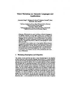
The test testRootModel sends 6 messages. The messages assert:, new, mooseID and > are directly sent by testRootModel. The message new sends basicNew and initialize. The total number of messages sent by testRootModel is 115. The message assert:, which belongs to the SUnit framework, does some checks on the argument and the method initialize is redefined in the class MooseElement. The number of messages can easily skyrocket. Running the tests associated with the Pharo collection library [10] takes slightly more than 32 seconds. The test execution sends more than 334 million messages. Linear regression. A scatter plot is drawn from our measurements (Figure 1). Each of the applications we have profiled is represented by a point (execution time, number of message sends) and is denoted with a cross in the scatter plot. The measurements execution time and number of message sends are the average of 10 successive executions. These values form an almost straight line with a statistical correlation of 0.99. The correlation is a general statistical relationship 8

Principally available from http://www.squeaksource.com

6

message sends

6

400 x 10 400000000 6

300 x 10 300000000 6

200 x 10 200000000 6

100 x 10 100000000

0

0

10000

20000

30000

40000

times (ms) Fig. 1. Linear regression for the 16 Pharo applications.

between two random variables and observed data values: a value of 1 means the data forms a perfect straight line. This line, commonly called regression line, may be deduced from these values. The general equation of a regression line is ˆy = a + bx where a is constant term; b is the line slope; x is the independent variable; y is the dependent variable; ˆy the predicted value of y for a given value of x. The independent variable is the execution time and the dependent variable is the number of message sends. We also put an additional constraint on the constant term: an execution time of 0 means that no message has been sent. Using the material provided in Appendix A, we estimate the sample regression line on our machine to be ˆy = 9 335.55 x, meaning that in the average, the virtual machine sends 9.3 million of messages per second. The line is drawn in Figure 1. We designate the average message rate (number of message sends per unit of time) as MRΓ,c where Γ is the set of the applications we profile and c the context in which the experiment has been realized. c captures all the variables that the measurements depends on (e.g., computer, RAM, method cache implementation, temperature of the room). We now have established the relation between the number of message sends and the execution time. We are not done yet however: only an approximation has been determined. The MRΓ,c value has been computed from an arbitrary set of applications. If we had chosen a different set of applications, say Γ 0 , MRΓ 0 ,c would have probably be slightly different from MRΓ,c . MRΓ,c is said to be a random variable, and it possesses a probability distribution. Assuming that the applications we have chosen are representative of the all possible applications available in Pharo, the real value of MRA,c , where A is the set of all Pharo applications, rests in an interval that is calculated according to how confident we want to be in our findings. 7

The standard deviation of error tells us how widely the errors are spread around the regression line. This value is essential to estimate the confidence interval that includes MRA,c . Appendix A details how the standard deviations (se and sb ) are computed. We have the standard deviation of error se = 16 448 897. The confidence interval is [MRΓ,c − t sb ; MRΓ,c + t sb ] where sb = 350.84 is the standard deviation of MRΓ,c and t is a value obtained from the standard t distribution table based on the confidence (1 − α) we want to have, with 1 (= 100%) being the most confident. For a 95% confidence interval, we have α = 0.05 and therefore t = 2.145 according to the standard t distribution, which may be found in any statistical text book. As a result, the confidence interval is [8 582, 10 089], which means that there is a probability of 95% that the real value MRA,c is within the interval. The linear regression model enables the prediction of the average execution time from the number of sent messages. Consider GitFS, an implementation of Git in Pharo. The tests of GitFS send 28 096 569 messages. According to the regression model, this corresponds to a period of time (28 096 569−418 253)/9 335.55 = 2 965. GitFS’ tests actually run in 2 928 milliseconds, which is included in the time interval [2 743, 3 225]. 3.2

Method invocation

One of the problems message counting is addressing is the poor stability and prediction of execution sampling. This section compares the stability of the execution time with the stability of number of sent messages, which answers the research question B. Hash values. Before we further elaborate on the precision of message counting, it is relevant to remark that executing the same code expression multiple times may not always send the same number of messages. For example, adding an element to a set does not always send the same number of messages. Consider the following code excerpt: |s| s := Set new. Compteur numberOfCallsIn: [ 1000 timesRepeat: [ s add: Object new ] ]

Line 2 creates a new set. Line 3 invokes our library by sending the message numberOfCallsIn: which takes a block as parameter (a block is equivalent to a

lambda expression in Scheme and Lisp and an anonymous inner class in Java). Line 4 creates 1000 entries in the set. The hash values of the key objects are used for the internal indexing of the set. The virtual machine generates the hash values and they cannot be predicted since they are based on a pseudo random number generator9 . Each execution of this piece of code gives a different value (e.g., 54 383, 55 997, 56 165) since the computation needed to add an object 9

In Cog, the jitted virtual machine, the hash is derived from the memory allocation pointer. The non-jitted VM produces a new hash value from a formula taking as input the previous generated hash value.

8

into a table depends on the object hash value pseudo-randomly provided by the virtual machine. Even though the way hash values are assigned to objects is indeed a source of non-determinism, as we will subsequently see, it has a low impact on our measurement: for the applications we have profiled, the number of message invocations varies significantly less than the execution time. Interactively acquiring data from the user, the filesystem or the network may also be another source of variation for the number of message sends.

Coefficient of variation. Each execution of the same piece of code results in a different execution time and a different number of messages sent. We will now assess whether the number of sent messages is a more stable metric than the execution time over multiple executions. For each of the 16 applications we executed its tests 10 times and calculated the standard deviation of execution time (sTimeTaken ) and number of sent messages (smessages ). To be able to compare these two standard deviations, we use the coefficient of variation, defined as the ratio of the standard deviation to the mean, resulting in ctime and cmessages , respectively. Appendix A gives our measurement and details how the variation is computed. For the 16 applications we considered, our result shows that the stability of the execution time (the ctime column) varies significantly from one application to another. For example, the applications ProfStef, Glamour and Magritte are relatively constant in their execution time. The variation may even be below 1% for ProfStef. However, execution time significantly changes at each run for a number of the applications. The execution time of XMLParser, DSM and PetitParser varies from 25% to 46%. The execution time of PetitParser may vary by 46% from one run to another. The reason for this is not completely clear. Private discussion with the author of PetitParser revealed the cause of this variation to be the intensive use of short methods on streams. These short methods, such as peek to fetch one character from a stream and next to move the stream position by one, have an execution time close to the elementary operations performed by the virtual machine to lookup the message in method cache10 . In contrast to execution time, message counting is a much more stable metric since its variation is usually below 1%. The greatest variation we have measured are with Mondrian and Moose. This is not surprising since these two applications intensively use non-deterministic data structures like sets and dictionaries to store their model. The average values of the normalized standard deviation of execution time ctime and cmessages are 13.95 and 0.61, respectively. For the experimental set up we have used, we have found that over multiple executions of the same piece of code, measuring the number of sent messages is 22.86 (13.95 / 0.61) times more stable than measuring the execution time. 10

The reason why fast messages cause the execution time to vary so much is not completely clear to us. We cannot reproduce this on micro-benchmarks. Additional analyses are required. We have left this as future work.

9

3.3

Effect of the execution context

We repeated the experiment on two additional execution platforms: on the MacBook Pro using the Cog virtual machine (which supports Just-In-Time compilation (JIT)) and a Linux Gentoo (2.6.34-gentoo-r6 running on an Intel Xeon CPU 3.06GHz GenuineIntel) using a non-jitted virtual machine. On the Cog virtual machine we have MRΓ,c0 = 58 384.75, with a 95% confidence interval [55 325, 64 123]. On this platform, the ratio between ctime and cmessages is 18.98. This is lower than what we obtained on the non-jitted virtual machine. The reason stems from the multiple method compilations, each being a resource-consuming process on its own. On the standard virtual machine running on Linux we obtained MRΓ,c00 = 12 412.34, with a 95% confidence interval of [9 615, 14 121]. The ratio between ctime and cmessages is 22.34, which corresponds to the ratio we have measured on the MacBook Pro without the JIT-ing VM. 3.4

Tracking optimizations

We identified a number of execution bottlenecks in the Mondrian visualization engine in our previous work [5]. We removed the bottlenecks by adding a “memoization” mechanism which is a common technique applied to methods free of side effects to avoid unnecessary recalculations. Memoizing the method MOGraphElement>> bounds improved Mondrian performance by 43%. Another memoization of MOGraphElement>> absoluteBounds resulted in a speedup of 45% (for the UI thread this time). Comparing the number of message sends with and without the optimization gives performance increases in the same range: the number of messages sent with the bounds optimization is 42% less than the non-optimized version and 44% for the absoluteBounds optimization. We have sequentially measured the logic thread then the UI thread. After having sampled the execution of the logic thread we had to restart the virtual machine to use the same initial state of the memory and the method cache. There was no need to restart the virtual machine between the two measurements when counting messages. No major conclusion can be drawn from this experiment. However, it emphasizes an important practical point. 3.5

Cost of counting messages

Counting the number of executed send bytecode instructions is cheap. We measure the execution time of each of the 16 applications with and without the presence of message counting. Table 3 reports our results. Each measurement is the average of 5 executions. The overhead is computed as overhead = (time on modified VM – time on normal VM) / time on normal VM * 100. The cost of message counting is almost insignificant. The execution time variation ranges from 0% to 0.02%. These results are not surprising actually. Message counting is simple to implement within the virtual machine; at each send bytecode a global variable is incremented. This is a cheap operation compared to the complex machinery to lookup method implementation, interpret the bytecode, and to manage the memory. The execution time variation we have measured on a non-jitted virtual machine is of the same range on Cog. 10

4

Counting Messages to Identify Execution Bottlenecks

CPU profilers aim at identifying methods that consume a large share of the execution time. These methods are likely to be considered for improvement and optimization, aiming at reducing the total program execution time. This section considers counting message as a means of finding runtime bottlenecks, and answers research question C. 4.1

A method as an execution bottleneck

A method is commonly referred as an execution bottleneck when it is perceived as taking a “lot of time”, or more time that it should. The intuition on which we will elaborate is that if a method is slow then it is likely to be sending (directly and indirectly) “too many” messages. Sending “too many” messages may not be the only source of slow down. An excessive use of memory and numerous invocations of the primitives offered by the virtual machine are likely to play a role in the time taken for a program to execute. A program that intensively uses files or the network may spend a significant amount of time executing the corresponding primitives. In Pharo, executing a primitive suspends the program execution and resumes it once the primitive has completed. Consider a program that sends few messages but makes a great use of primitives: the program can take a long time to execute with few sent messages. However, we have not detected such occurrence in all the applications we studied. As we will see in the coming sections, in spite of the perturbation that may be introduced by primitive executions, still make message counting more advantageous than execution sampling for all the applications we have considered. 4.2

Method invocations per method

Counting the number of messages sent by a particular method is an essential step to compare execution sampling with message counting. Counting the number of sent messages for each method requires associating with each method the number of messages it sends at each execution. Most code instrumentation libraries and tools, including most aspect-oriented programming ones, easily meet this requirement. The instrumentation we consider for each method of the application to be profiled is done as follows. CompteurMethod>> run: methodName with: listOfArguments in: receiver | oldNumberOfCalls v | oldNumberOfCalls := self getNumberOfCalls. v := originalMethod valueWithReceiver: receiver arguments: listOfArguments. numberOfCalls := (self getNumberOfCalls - oldNumberOfCalls) + numberOfCalls - 5. ˆ v

Compteur is the implementation of our message-based code profiler for Pharo. An instance of the class CompteurMethod is associated with each method of the application to be profiled. CompteurMethod acts as a method wrapper by 11

intercepting each method invocation. At each method invocation, the method run:with:in: is executed to increase the variable numberOfEmittedCalls defined in the CompteurMethod instance. The number of executions of a method is associated with the method itself. Note that we do not instrument the whole system, but just the application we are interested in profiling. The method getNumberOfCalls uses a primitive operation defined in the virtual machine to obtain the current number of message sends. The instrumentation itself sends 5 messages: valueWithReceiver:arguments:, withArgs:executeMethod: and the second getNumberOfCalls, plus 2 messages sent by valueWithReceiver:arguments:, not presented here. We therefore need to subtract 5 from the number of calls. 4.3

Method execution time and number of message sends

number of method invocations

The total execution time of an individual method is correlated with the number of messages that are directly and indirectly sent by the method. In this section, we focus on a single application, Mondrian. Other applications enjoy the correlation.

6

10.0 x 10 10000000 6

7.5 x 10 7500000 6

5.0 x 10 5000000 6

2.5 x 10 2500000 0

0

75

150

225

300

time (ms)

Fig. 2. Linear regression for the methods of Mondrian.

Figure 2 plots the methods of the Mondrian application according to their execution time in milliseconds with the number of sent messages. Note that we consider the total execution time and the total number of message sends for each method, counting the closure of all of the methods that it invokes. This means that if a method is invoked 100 times for which each execution takes 2 ms and sends 5 messages, then the method is plotted as the point (200, 500). The graph shows that the time taken by the computation that is initiated by sending a message is almost constant: the execution time of a method is directly proportional to the number of messages that it sends. 12

As with application execution (Section 3.1), the regression model indicates that the large majority of (execution time, number of message sends) plots form a straight line (Figure 2), confirmed by a correlation of 0.97. The equation of the regression line is ˆy = 31 811.38 x. Figure 2 gives this line. We see that the slope of the regression line is about 3.4 greater than the slope we found when we studied application executions (Section 3.1). The reason stems from the cumulative effect of nested message sends. To get a feeling why this happens, consider the following two methods: MOGraphElement>> bounds | basicBounds | boundsCache ifNotNil: [ ˆ boundsCache ]. self shapeBoundsAt: self shape ifPresent: [ :b |ˆ boundsCache := b ]. ... MONode>> startPoint ˆ self bounds bottomCenter

The method bounds sends 239 direct and indirect messages. The method startPoint sends 2 direct messages. But since it invokes bounds and bottomCenter (which sends 27 messages), in total, startPoint sends 2 + 27 + 239 = 268 messages. 4.4

Stability of message counting

To assess the stability of message counting over execution sampling we will compare a list of profiles made with message counting and execution sampling. The idea is to numerically assess the variability of the method ranking against multiple profiles of the same code execution. We will then characterize a stable set of profiles with a constant method ranking. Stability of profiles. We have profiled Mondrian 20 times: 10 using execution sampling and 10 using message counting. Each profile is obtained by running the unit tests and provides a ranking of the methods. Methods are ranked in order of “computational cost”. To save space, Table 1 gives only an excerpt of our measurements: the first 9 methods (names have been shortened to m1...m9) are ranked for 5 profiles. The method ranked first is the one that has the greatest share of the CPU execution time; the method ranked last is the one that has consumed the least CPU. The 5 profiles are obtained with MessageTally. As stated earlier (Section 2), due to the high sensitivity of the environment, not all the rankings are the same. Quantifying the variation of the method ranking for a set of profiles is the topic of this section. For each method, we compute the standard deviation of the ranking (ses ) to estimate ranking variability. We have ses (m) = 0 if the method m is always ranked the same across the profiles. The greater ses is, the greater the variability of the ranking. The stability of a set of profiles depends on the variability of the method ranking. However, not all methods deserve to be considered in the same way. We use the discounted cumulated gain [13] to weight the ranking. The point of 13

m1 m2 m3 m4 m5 m6 m7 Profile 1 1 2 3 4 5 6 7 Profile 2 1 2 3 4 6 5 10 Profile 3 1 2 3 4 6 5 10 Profile 4 1 2 3 4 5 6 9 Profile 5 1 2 3 5 6 4 9 Average 1 2 3 4.1 5.4 5.5 8.9 Stand. Dev. ses 0.000 0.000 0.000 0.316 0.516 0.707 1.197

m8 8 12 12 7 12 10.4

m9 9 7 7 13 7 8.2

1.955 1.989

Table 1. Ranking of the first 9 methods of Mondrian for 5 profiles (execution sampling).

a weight is that the lower the ranked position of a method, the less valuable it is for the user, because the less likely it is that the user will ever consider the method as being slow. A discounting function is needed which progressively reduces the method score as its position in the ranking increases. We weight a method ranked n as w(n) = 1/ln (n + 1). We P define the instability for the first n n methods of the set of profiles P as ψ n (P ) = i=1 ses (i) ∗ w(n), the sum of the weighted standard deviations. According to the excerpt given in Table 1, we have ψ 9 (P ) = 0 1 + ... + 0.316 1 + 0.516 1 + ... + 1.989 1 = 3.177. ln(1+1) ln(4+1) ln(5+1) ln(9+1) A perfectly stable set of profiles P has the value ψ(P ) = 0. Experimental setting. We have profiled each application γ 20 times in the execution context c. We have γ ∈ Γ , where Γ is the list of applications given in Appendix A. 10 of these profiles were obtained using the standard execution sampling. We refer to these 10 profiles as Pγ,c . As mentioned earlier, the execution context in which the applications are profiled is c. The 10 remaining profiles were obtained using message counting, referred as Qγ,c . We have chosen to consider the same number of methods for each application since not all the applications have the same code size. As previously described, we ran the unit tests to produce the profiles. Poor stability of execution sampling. The method ranking against the execution time is not constant: each new profile gives a slightly different method ranking. For example, for 8 of the 10 profiles of PPetitParser,c , the method ranked 5th in terms of execution time is PPPredicateTest>> testHex. However, in the 2 remaining profiles, this method is ranked 35 and 36 (!). After an examination of the tests to make sure they do not randomly generate data, we speculate that this odd ranking is due to a mixture of the problems highlighted at the beginning of this article (Section 2). This kind of variability in the method ranking is hardly avoidable, even though we took great care to garbage collect the memory and release unwanted object references between each profile. We define ψ 10 (Pγ,c ) over the first 10 methods given by a set of profiles P for an application γ realized in an execution context c. To give a reference point, we artificially build a random data set R on which we can compare ψ of the 14

applications we profile: we randomly generate 10 random rankings. For our random set of profiles, we have ψ 10 (R) = 173 and ψ 10 (PPetitParser,c ) = 11. All the remaining ψ 10 range from 3 to 5. The greatest instability of the set of profiles we obtained is for PetitParser. PetitParser makes heavy uses of stream and string processing, which perturbs MessageTally, the standard execution sampling profiler of Pharo, for the same reasons mentioned in Section 3.2 (use of short methods). Perfect stability of message counting. The profiles obtained with message counting have a ψ of 0 for each of the applications we have profiled. This means that the 10 profiles we made for each application do not show a variation in the method ranking according to the number of sent messages. Even though we have seen that the number of method invocations varies slightly (Section 4.2), the data we collected from this experiment show that this does not impact the method ranking. Profiling multiple times always ranks the methods identically. The stability execution sampling does not equal that of message counting. The stability of message counting is clearly superior to that of execution sampling.

4.5

Cost of the instrumentation

Determining the number of sent messages for each method requires complete instrumentation of the application to be profiled. This instrumentation introduces an overhead. The cost of the instrumentation depends on the infrastructure used for code transformation. We used the Spy framework [4]. To evaluate our implementation, we performed two set of measurements. For each application, we ran its associated unit tests twice, with and without the instrumentation. Table 4 presents our results.

Overhead (%)

Overhead (%)

3000

10000

2250

1000

1500

100

750

10

0

0

10000

20000

30000

40000

Execution time (ms) (a) Linear scale

1

0

10000

20000

30000

(b) Logarithmic scale

Fig. 3. Ratio between overhead and execution time.

15

40000

Execution time (ms)

Running the unit tests while counting message sends for each method has an overhead that ranges from 2% to 2 524%. This overhead includes the time taken to actually instrument and uninstrument the application. When the unit test takes a short time to execute, then the instrumentation may have a high cost. The worst cases are with XMLParser and AST. AST’s unit tests take 37 ms to execute. They take 971 ms with the instrumentation, representing an overhead of 2 524%. The AST package is composed of 76 classes and 1 246 methods. XMLParser’s unit tests take 36 ms to execute. The package is composed of 47 classes and 785 methods. Since XMLParser is smaller than AST, the overhead of the instrumentation is also smaller. Figure 3 represents the ratio of the overhead to the test execution time. The left hand-side presents this ratio with a linear scale. The right-hand side gives the same data, with a logarithmic scale for the overhead. Each cross is a pair (execution time, overhead), representing an application. Figure 3 shows a general trend: the longer the unit tests take to execute, the smaller the instrumentation overhead. Above an execution time of approximately 5 seconds, determining the number of message sends per method has an overhead of less than 100%, which represents twice the execution time of the unit tests. In practice, this is acceptable in most of the situations we have experienced. DSM has an overhead of 2.4%, the smallest overhead we measured. The reason for this low overhead is that most of the logic used by the DSM package is actually implemented in Famix, a different package. When DSM is the only package instrumented, the overhead is low since most of the work happens in a different package, itself uninstrumented. Note that the execution time of the tests and the cost of the instrumentation are unrelated. This is because the execution time of the tests depends on how much logic is executed to complete tests, and not on how much of that execution is attributable to the execution package.

5

Contrasting Execution Sampling with Message Counting

We revisit the issues encountered with execution sampling that we previously enumerated (Section 2) and contrast them with the message counting technique described above. No need for sampling. Message counting provides an exact measurement of a particular execution. The measurement is solely obtained by counting the number of message sends. Message counting therefore does not depend on thread support or advanced reflective facilities (e.g., MessageTally heavily relies on threads and runtime call stack introspection) or sophisticated support of the virtual machine (e.g., the JVM offers a large protocol for profiling agents). As described in Section 6, adapting a non-jitted virtual machine to count send instructions may require adding a few dozen lines of code. Execution environment. Message counting is not influenced by the thread scheduling or memory management. The benefit is that we are able to compare profiles 16

obtained from different execution environments. For the applications we have considered, sending messages is correlated with the average execution time. As we have shown, this means that the average execution time can be easily approximated from the number of messages. Stable measurements. Measurements obtained from message counting are significantly more stable than those obtained from execution sampling. Even though the exact number of message sends may vary over multiple executions (partly due to the hash values given by the virtual machine), the metric is stable and reproducible in practice. Profiling time. Contrary to execution sampling, message counting is well adapted to short profiles since an exact value is always returned. One compelling application of this property is asserting upper bounds on message counts when writing tests. We have produced an extension of unit test that offers a new kind of assertion: assertIs:fasterThan: to compare the number of messages sent. We have written a number of tests that define time execution invariant. One example for Mondrian is (the difference between the two executions is shown in bold): MondrianSpeedTest>> testLayout2 | view1 view2 | ”All the subclasses of Collection” view1 := MOViewRenderer new. view1 nodes: (Collection allSubclasses). view1 edgesFrom: #superclass. view1 treeLayout. ”Collection and all its subclasses” view2 := MOViewRenderer new. view2 nodes: (Collection withAllSubclasses). view2 edgesFrom: #superclass. view2 treeLayout. self assertIs: [ view1 root applyLayout ] fasterThan: [ view2 root applyLayout ]

The code above says that computing the layout of a tree of n nodes is faster than with n + 1 nodes. The difference between these two expressions is just the message sent to Collection. Being able to write a test for short execution time is a nice application of message counting. As far as we are aware, none of the mainstream testing frameworks is able to define assertions to compare execution times.

6

Implementation

Compteur is an implementation of the message-counting mechanism for Pharo. It comprises a new virtual machine and a profiler based on the Spy profiling framework [4]. The modification made in the virtual machine is lightweight: a global variable initialized to 0 is incremented each time a send bytecode is interpreted. In the 17

non-jitted Pharo virtual machine, the increment is realized in the part of the bytecode dispatch switch dedicated to interpret message sending. In the jitted Cog virtual machine, the preamble of the method translated in machine code by the JIT compiler realizes the increment. The maximum value of a small integer in Pharo is 230 (∼ 1.073 ∗ 109 ). Over this value, an integer is represented as an instance of the LargeInteger class, which is slow to manipulate within the virtual machine. The current Pharo virtual machine (5.7beta3) executes approximately 12 M message sends per second on micro benchmarks11 . This means that the range of the Pharo integer values may be exhausted after 90 seconds (1 073 / 12). Using a 64 bit integer is not an option since Pharo is designed to run on 32 bit machines. We therefore use two small integers to encode the number of sent messages. The maximum number of messages that can be counted in this way is ∼ 1.152 ∗ 1018 . Even at full interpretation speed, this value is not reached after 2 million hours. The global message counter is made accessible within our profiler written in Pharo via primitives. The counter is reset via a dedicated primitive. The instrumentation is realized by wrapping methods to intercept incoming messages [4]. To obtain the number of message sends per method, the application has to be instrumented to capture the value of the global counter before and after executing the method, as illustrated in Section 4.2. Using the Aspect-OrientedProgramming terminology, such instrumentation is easily realized with around or before and after advice.

7

Discussion

The design of our approach is the result of a careful consideration of various points. Modifying the virtual machine. Even though the modification we made in the virtual machine is relatively lightweight, we are not particularly enthusiastic about producing a new virtual machine since the Pharo community is not particularly keen on changing the virtual machine. People are often reluctant to use non-standard tools, even if the benefits are strong and apparent. We have not found a satisfactory alternative. As an initial attempt, before we implemented the work presented in this paper, we made a profiler that counted only the messages sent by the application, and not by dependent libraries and the runtime. The application was instrumented by code modification and the virtual machine was left unmodified. We discovered that the information we gathered was insufficient to demonstrate the properties presented in this paper. As soon as the execution flow leaves the application, no information is recorded until it returns to the application. Since it cannot be accurately predicted how long the execution flow will spend outside the application, we could not establish a correlation between the number of messages sent by the application and execution time. 11

Result of the standard 0 tinyBenchmarks micro benchmark.

18

Instrumentation. Our approach requires instrumentation of the application to be profiled: only the methods defined in the application we wish to improve need to be instrumented. Instrumenting the complete system has not proven to be particularly useful or possible in our situation: (i) if an execution slowdown is experienced, there is no need to look for its cause outside the application we are actually considering; (ii) instrumenting the whole system has a significant runtime cost; (iii) this easily leads to meta-circularity issues since our profiler shares the runtime with the profiled application. Even if recent advances in instrumentation scoping are adopted [24], this increases the complexity of the implementation without a clear benefit. Efficiently handling metacircularity is necessary to profile the profiler itself. However, since the implementation of Compteur is not particularly complex, we have not felt the need to do so. Special messages. For optimization purposes, not all messages are sent in Pharo. Depending on the name of the message being sent, the Pharo compiler may decide to transform the message send into a particular sequence of bytecode instructions. Consider the message ifTrue:ifFalse: with literal two block arguments. For example, the expression (1 < 2) ifTrue: [ ’Everything is okay’] ifFalse: [ ’Something is wrong’ ] is translated into the sequence: 76 pushConstant: 77 pushConstant: B2 send: < 99 jumpFalse: 27 21 pushConstant: 90 jumpTo: 28 20 pushConstant: 87 pop 78 returnSelf

1 2

’Everything is okay’ ’Something is wrong’

Beside ifTrue:ifFalse:, there are other 17 control flow instructions treated as “special messages” by the Pharo compiler. In the Pharo virtual machine, a jump bytecode is faster than a send. In the whole Pharo library, approximately 62% of all message sends contained in the source code are translated into send bytecode instructions. The correlation we established between execution time and message sends is strong, even if 38% of message sends are not translated into send bytecode instructions. We obtained these figures by comparing for each method in Pharo the abstract syntax tree of the source code and the generated bytecode instructions. The case of primitives. The execution time of a method may have little relation to the number of messages sent. This could happen if the method intensively uses primitives, or if the program had to wait for a keystroke. The profile of such a program then depends on how long the user has waited before pressing a key. We reasonably assume that this is not what happens in practice: we chose unit tests as the execution reference, which is a realistic approximation of a program execution. 19

Particularities of Pharo. Pharo’s compiler is rather simplistic, not designed for producing optimized bytecode. It does not offer additional optimization than a mere bytecode generation pattern based on the name (e.g., ifTrue:ifFalse:, timesRepeat:), as previously mentioned. Pharo memory layout is based on a generational and compacting mark and sweep. Virtual memory file mapping is supported and the virtual machine has the ability to grow and shrink the memory space. Are our results applicable to other dynamic languages? At first glance, Jython12 , JRuby13 , Groovy14 enjoy the same nice properties as Pharo: the computation is solely realized via sending messages. It is therefore tempting to extrapolate our results to these languages. However, the Java Virtual Machine, which is the execution platform of these languages, has a radically different execution model. For example, the JVM has native threads which have an impact on the memory management. Pharo has “green threads”: the scheduler is implemented in Pharo itself. Most implementations of the JVM garbage collector have many more generations than the one of Pharo: Pharo supports only 2 generations (young and old) whereas the HotSpot Java VM has 5 memory pools. Last but not least, the heavy optimization of the JVM just-in-time compiler has the potential to completely invalidate our finding. Testing whether our results are applicable to other “pure OO” languages implies further analysis and measurements.

8

Related Work

The work presented in this paper is not the first attempt at finding an alternative to execution sampling. However we are not aware of any work which studied the number of message sends. Bytecode instruction counting. Camesi et al. [6] pioneered the field by investigating the use of bytecode instruction counting as an estimate of real CPU consumption. For all the platforms they have considered, there is an application-specific ratio of bytecode instructions per unit of CPU time. Such a bytecode ratio can be used as a basis for translating a bytecode instruction value into the corresponding CPU consumption. Out results are similar. We have also identified a message ratio, however this ratio is attached to a particular execution platform, and not to an application. Dynamic bytecode instrumentation. Instrumentation-based profiling has a high cost. However, such overhead can be reduced by instrumenting only the subset of the application where a bottleneck is known to be. Dmitriev [8] proposes that for a given set of arbitrary “root” methods, instrumentation applies to the call subgraph of the roots only. Dmitriev observed that this approach generally works much better for large applications, than for small benchmarks. The reason is that additional code and data become negligible once the size of the profiled application 12 13 14

http://www.jython.org http://jruby.codehaus.org http://groovy.codehaus.org

20

goes above a certain threshold. Message counting has similar properties. Only a subset of the system needs to be instrumented. However, message counting behaves perfectly well for small benchmarks. Hardware Performance Counters. Most modern processors have complex microarchitectures that dynamically schedule instructions. These processors are difficult to understand and model accurately. For that purpose, they provide hardware performance counters [1]. For example, Sun’s UltraSPARC processors count events such as instructions executed, cycles expended and many more. With message counting we exploit the same kind of information, but obtained from the Pharo virtual machine. Optimizing Smalltalk. The popularity of Smalltalk during the 80’s has led to numerous works that directly tackled the slow execution of Smalltalk programs. Sophisticated mechanisms on mapping bytecode to instruction machine [23,25], improved compiled methods and cache contexts [19], manipulating method dictionaries [3] and adding type declaration and inference [2,14] have been produced.

9

Conclusion

A code profiler provides high-level snapshots of a program execution. These snapshots are often the only way to identify and understand the cause of a slow execution. Whereas execution sampling is a widely used technique among code profilers to monitor execution at a low cost, it brings its own limitations, including non-determinism and inability to relate profiles obtained from different platforms. We propose counting method invocations as a more advantageous profiling technique for Pharo. We have shown that having method invocation as the exclusive computational unit in Pharo makes it possible to correlate message sending and average execution time with stability, both for applications as a whole and for individual methods. We believe that code profiling has not received the attention it deserves: execution sampling uses stack frame identifiers, which essentially ignore the nature of object-oriented programming. In general, code profilers profile object-oriented applications pretty much the same way that they would profile applications written in C. We hope the work presented in this paper will stimulate further research of the field to give more importance to objects than to low-level implementation considerations. Acknowledgment. We thank Mircea Lungu, Oscar Nierstrasz, Lukas Renggli and Romain Robbes for the multiple discussions we had and their comments on an early draft of the paper. We particular thank Walter Binder for his multiple discussions and advices. Our thanks also go to Eliot Miranda for his help on porting Compteur to Cog, the jitted virtual machine of Pharo. We thank Gilad Bracha and Jan Vran´ y for the fruitful discussions we had. We also thank Andrew P. Black for his precious help on improving the paper. We gratefully thank Mar´ıa Jos´e Cires for her help on the statistical part. We also thank ESUG, the European Smalltalk User Group, for its financial contribution to the presentation of this paper.

21

References 1. Glenn Ammons, Thomas Ball, and James R. Larus. Exploiting hardware performance counters with flow and context sensitive profiling. In Proceedings of PLDI’97, pages 85–96, ACM. 2. Robert G. Atkinson. Hurricane: An optimizing compiler for Smalltalk. In Proceedings OOPSLA’86, pages 151–158, ACM. 3. S. Baskiyar. Efficient execution of pure object-oriented programs by follow-up compilation. Computing, 69:273–289, December 2002. 4. Alexandre Bergel, Felipe Ba˜ nados, Romain Robbes, and David R¨ othlisberger. Spy: A flexible code profiling framework. In Smalltalks 2010. To appear. 5. Alexandre Bergel, Romain Robbes, and Walter Binder. Visualizing dynamic metrics with profiling blueprints. In Proceedings of TOOLS EUROPE’10, pages 291–309. Springer. 6. Andrea Camesi, Jarle Hulaas, and Walter Binder. Continuous bytecode instruction counting for cpu consumption estimation. In Proceedings of the 3rd international conference on the Quantitative Evaluation of Systems, pages 19–30, 2006, IEEE. 7. Amer Diwan, Han Lee, and Dirk Grunwald. Energy consumption and garbage collection in low-powered computing. Cu-cs-930-02, University of Colorado, 2002. 8. M. Dmitriev. Profiling java applications using code hotswapping and dynamic call graph revelation. In Proceedings of the Fourth International Workshop on Software and Performance, pages 139–150, ACM, 2004. arli, Roel Wuyts, and Andrew P. 9. St´ephane Ducasse, Oscar Nierstrasz, Nathanael Sch¨ Black. Traits: A mechanism for fine-grained reuse. TOPLAS, 28(2):331–388, ACM, March 2006. 10. St´ephane Ducasse, Damien Pollet, Alexandre Bergel, and Damien Cassou. Reusing and composing tests with traits. In Proceedings of TOOLS EUROPE’09, pages 252–271, Springer. 11. David Freedman, Robert Pisani, and Roger Purves. Statistics, Third Edition. W. W. Norton & Company, 1997. 12. Aloke Gupta and Wen-Mei W. Hwu. Xprof: profiling the execution of X Window programs. In Proceedings of joint international conference on Measurement and modeling of computer systems, SIGMETRICS ’92/PERFORMANCE ’92, pages 253–254, ACM. 13. Kalervo J¨ arvelin and Jaana Kek¨ al¨ ainen. Cumulated gain-based evaluation of ir techniques. ACM Trans. Inf. Syst., 20(4):422–446, October 2002. 14. Ralph Johnson. TS: An optimizing compiler for Smalltalk. In Proceedings of OOPSLA ’88, pages 18–26, ACM. 15. L. Kleinrock and R. R. Muntz. Processor sharing queueing models of mixed scheduling disciplines for time shared system. J. ACM, 19(3):464–482, July 1972. 16. Prem S. Mann. Introductory Statistics. Wiley, 2006. 17. Robert Cecil Martin. Agile Software Development. Principles, Patterns, and Practices. Prentice-Hall, 2002. 18. Michael Meyer, Tudor Gˆırba, and Mircea Lungu. Mondrian: An agile visualization framework. In Proceedings of Symposium on Software Visualization (SoftVis’06), pages 135–144, ACM. 19. Eliot Miranda. Brouhaha — A portable Smalltalk interpreter. In Proceedings of OOPSLA ’87 pages 354–365, ACM. 20. Todd Mytkowicz, Amer Diwan, Matthias Hauswirth, and Peter F. Sweeney. Producing wrong data without doing anything obviously wrong! In Proceeding of the 14th international conference on Architectural support for programming languages and operating systems, ASPLOS ’09, pages 265–276, ACM.

22

21. Todd Mytkowicz, Amer Diwan, Matthias Hauswirth, and Peter F. Sweeney. Evaluating the accuracy of java profilers. In Proceedings of PLDI ’10, pages 187–197, ACM. 22. Todd Mytkowicz, Amer Diwan, and Elizabeth Bradley. Computers Are Dynamical Systems. Chaos, 19:033124, 2009. 23. A. Dain Samples, David Ungar, and Paul Hilfinger. SOAR: Smalltalk without bytecodes. In Proceedings of OOPSLA ’86, pages 107–118, ACM. ´ 24. Eric Tanter. Execution levels for aspect-oriented programming. In Proceedings of AOSD’10, pages 37–48, ACM. 25. David Ungar, David Patterson Smalltalk-80: Bits of History, Words of Advice Berkeley Smalltalk: Who Knows Where the Time Goes? In Smalltalk-80: Bits of History, Words of Advice, pages 189–206, Addison-Wesley, 1983. 26. Jia Yu, Jun Yang, Shaojie Chen, Yan Luo, and Laxmi Bhuyan. Enhancing network processor simulation speed with statistical input sampling. In Proceedings of High Performance Embedded Architectures and Compilers, volume 3793 of LNCS, pages 68–83, Springer, 2005.

A

Linear Regression Material

This section contains the relevant data and theoretical tools to construct the regression linear model described in Section 3.1 and Section 4.3. Measurements. Table 2 lists 16 Pharo applications. Each of these applications covers a particular aspect of the Pharo library and runtime. Collections is an intensively used library to model collections. Mondrian, Glamour and DSM make an intensive use of graphical primitives and algorithms. Nile is a stream library based on Traits [9]. Moose is a software analysis platform which deals with large models and files. Mondrian and Moose heavily employ hash tables as internal representation of their models. SmallDude, PetitParser, XMLParser heavily manipulate character strings. Magritte and Famix are meta-models. ProfStef intensively makes use of reflection. Network uses primitive in the virtual machine. ShoutTest and AST heavily parse and manipulate abstract syntax trees. Arki is an extension of Moose that performs queries over large models. These applications cover the features of Pharo that are intensively used by the Pharo communities: most of the applications are either part of the standard Pharo runtime or are among the 20 most downloaded applications. Not all the set of primitives offered by the virtual machines are covered by the applications. For example, none of them makes use of sound. We are not aware of any application that intensively uses Pharo’s musical support. For each of these applications, we report the mean execution time over 10 trials to run its corresponding unit tests (time taken (ms)) and the number of sent messages (# sent messages). These reported results are averages over 10 runs. For each of these two measurements, we compute the standard deviations (smessages and sTimeTaken , not reported here) and normalize it yielding ctime = sTimeTaken ∗100/TimeTaken and cmessages = smessages ∗100/messages. These applications were run on a virtual machine modified to support our message counting mechanism. The source code of each of these applications is available online on SqueakSource. 23

Application time taken (ms) # sent messages ctime % cmessages % Collections 32 317 334 359 691 16.67 1.05 Mondrian 33 719 292 140 717 5.54 1.44 Nile 29 264 236 817 521 7.24 0.22 Moose 25 021 210 384 157 24.56 2.47 SmallDude 13 942 150 301 007 23.93 0.99 Glamour 10 216 94 604 363 3.77 0.14 Magritte 2 485 37 979 149 2.08 0.85 PetitParser 1 642 31 574 383 46.99 0.52 Famix 1 014 6 385 091 18.30 0.06 DSM 4 012 5 954 759 25.71 0.17 ProfStef 247 3 381 429 0.77 0.10 Network 128 2 340 805 6.06 0.44 AST 37 677 439 1.26 0.46 XMLParser 36 675 205 32.94 0.46 Arki 30 609 633 1.44 0.35 ShoutTests 19 282 313 5.98 0.11 Average 13.95 0.61

Table 2. Applications considered in our experiment (second and third columns are average over 10 runs)

Estimating the sample regression line. For sake of completeness and providing easy-to-reproduce results, we provide the necessary statistical material. Complementary information may be easily obtained from standard statistical books [11]. For the least squares regression line ˆy = a+b x, we have the following formulas for estimating a sample regression line: b=

SSxy SSxx

a=y−b x

where y and x are the average of all y values and x values, respectively. The y variable corresponds to the # sent messages column and x to time taken (ms) in the table given above. P P P X X ( x)2 ( x)( y) 2 SSxx = x − SSxy = xy − n n where n is number of samples (i.e., 16, the number of applications we have profiled). SS stands for “sum of squares.” The standard deviation of error for the sample data is obtained from: rP P X SSyy − b SSxy ( y)2 se = where SSyy = y2 − n−2 n In the above formula, n − 2 represent the degrees of freedom for the regression se model. Finally, the standard deviation of b is obtained with sb = √SS . xx

24

Application Normal VM (ms) Compteur (ms) overhead (%) Collections 32 317 32 323 0.02 Mondrian 33 719 33 720 0 Nile 29 264 29 267 0.01 Moose 25 021 25 023 0.01 SmallDude 13 942 13 944 0.01 Glamour 10 216 10 218 0.02 Magritte 2 485 2 485 0 PetitParser 1 642 1 642 0 Famix 1 014 1 015 0.1 DSM 4 012 4 013 0.02 ProfStef 247 247 0 Network 128 128 0 AST 37 38 2.7 XMLParser 36 36 0 Arki 30 30 0 ShoutTests 19 19 0

Table 3. Cost of the Virtual Machine Modification

Application No inst (ms) Inst. (ms) overhead (%) Collections 32317 33590 3.94 Mondrian 33719 36983 9.68 Nile 29264 36387 24.34 Moose 25021 26652 6.52 SmallDude 13942 24467 75.49 Glamour 10216 12976 27.02 Magritte 2485 4361 75.51 PetitParser 1642 2102 28.01 Famix 1014 3327 228.07 DSM 4012 4108 2.40 ProfStef 247 562 127.47 Network 128 875 583.87 AST 37 971 2524.00 XMLParser 36 559 1452.78 Arki 30 236 685.71 ShoutTests 19 40 111.76

Table 4. Cost of the Application Instrumentation

25