Oct 16, 2015 - erators are of fundamental importance [Ar, B, CZ, D, M, S], and generalize the ... of the University of Missouri, and by the Simons Foundation. ..... Proposition 2.52] gives rise to the spectral flow argument essential for the ...
arXiv:1510.05015v1 [math.SP] 16 Oct 2015
COUNTING SPECTRUM VIA THE MASLOV INDEX FOR ONE ¨ DIMENSIONAL θ−PERIODIC SCHRODINGER OPERATORS CHRISTOPHER K. R. T. JONES, YURI LATUSHKIN, AND SELIM SUKHTAIEV Abstract. We study the spectrum of the Schr¨ odinger operators with n × n matrix valued potentials on a finite interval subject to θ−periodic boundary conditions. For two such operators, corresponding to different values of θ, we compute the difference of their eigenvalue counting functions via the Maslov index of a path of Lagrangian planes. In addition we derive a formula for the derivatives of the eigenvalues with respect to θ in terms of the Maslov crossing form. Finally, we give a new shorter proof of a recent result relating the Morse and Maslov indices of the Schr¨ odinger operator for a fixed θ.
1. introduction Relations between the spectral count and conjugate points for differential operators are of fundamental importance [Ar, B, CZ, D, M, S], and generalize the classical Sturm Theorem saying that the number of negative eigenvalues of the one dimensional scalar differential operator is equal to the number of conjugate points, that is, the zeros of the eigenfunction corresponding to the zero eigenvalue. In the matrix valued or multidimensional case the conjugate points are understood as the points of intersection of a path in the space of Lagrangian planes with the train of a fixed plane determined by the boundary conditions associated with the differential operator. The signed count of the conjugate points is called the Maslov index [Ar, BF, CLM, F]. Recently the relation between the spectral count and the Maslov index attracted much attention [BM, DJ, DP, CJLS, CJM1, CJM2, CDB1, CDB2, PW]. In particular, formulas relating the number of the negative eigenvalues of the Schr¨odinger operators with periodic potentials and the Maslov index were given in [JLM, LSS]. In this paper we continue this latter work but give it a new spin using θ as a parameter generating the path of the Lagrangian planes. The Schr¨odinger operator H = −∂x2 + V with a periodic potential V on R can be represented as the direct integral of θ−periodic Schr¨odinger operators Hθ on [0, 2π], see [ReSi, Section XIII]. This construction gives rise to the decomposition of the spectrum Spec(H) = ∪∞ k=1 [αk , βk ] into the union of spectral intervals [αk , βk ], with the end points αk , βk being equal to the k−th eigenvalue of the operator with either periodic or anti-periodic boundary conditions. Thus the properties of each fiber operator Hθ and its eigenvalues are of great interest. A natural question in this Date: October 20, 2015. Key words and phrases. Schr¨ odinger equation, Hamiltonian systems, eigenvalues, stability, differential operators, discrete spectrum. Supported by the NSF grant DMS-1067929, by the Research Board and Research Council of the University of Missouri, and by the Simons Foundation. We thank Graham Cox, Gregory Berkolaiko, and Alim Sukhtayev for discussions. Our special thanks go to Jared Bronski for asking if the parameter θ can be used to compute the Maslov index, and to Fritz Gesztesy for help. 1
C. JONES, Y. LATUSHKIN, AND S. SUKHTAIEV
s ✻
θ ✻ eigenvalues
θ2
s
Γ4
Γ2
eigenvalues
λ∞
Γ1
s s
s
θ1
✲λ
r
I
no intersections
Γ3
conjugate points
no intersections
s s
s
eigenvalues
s
Γ3
1
s
s s Γ4
Γ2
eigenvalues Γ1
∞
λ
II
s
conjugate points
2
τ
✲λ
0 r
Figure 1. context is how certain quantitative characteristics of Hθ , such as the Morse index Mor(Hθ ) = N (0, θ) or, more generally, the eigenvalue counting function N (r, θ), vary with respect to the parameter θ. We address these questions by employing methods of symplectic geometry. Let [a, b] be a finite interval and V ∈ L∞ ([a, b], Rn×n ) be symmetric a.e., and consider the eigenvalue problem for the operator Hθ := (−∂x2 )θ + V defined in (2.1)-(2.3), that is, the boundary value problem − u′′ (x) + V (x)u(x) = λu(x), λ ∈ R, x ∈ [a, b], u = (u1 , . . . , un ) ∈ Cn , iθ
′
iθ ′
u(b) = e u(a), u (b) = e u (a), θ ∈ [0, 2π).
(1.1) (1.2)
Problem (1.1),(1.2) can be reformulated in terms of existence of conjugate points. A pair of numbers (λ, θ) ∈ R × [0, 2π) is called a conjugate point if the subspace Fλ2 ⊂ C4n consisting of the Dirichlet and Neumann boundary traces of solutions to the second order equation (1.1) has a nontrivial intersection with the set Fθ1 := {(P, eiθ P, −Q, eiθ Q)⊤ : P, Q ∈ Cn }. By varying θ between the given values θ1 < θ2 in [0, π], and the spectral parameter λ between λ∞ , the uniform lower bound for the spectrum of Hθ , and some fixed number r > λ∞ , we obtain a loop γ in the set of Lagrangian planes in R16n . Each intersection of this loop with the diagonal plane {(p, p) : p ∈ R8n } gives a conjugate point. The total number of the conjugate points, corresponding to the part of the loop where θ = θ1 (respectively, θ = θ2 ), is equal to the number of the eigenvalues of Hθ1 (respectively, Hθ2 ) located below r. Using the homotopy invariance property of the Maslov index, one concludes that the total number of conjugate points (counting their signs) is equal to zero. Therefore the difference between the eigenvalue counting functions for Hθ1 and Hθ2 can be evaluated via the Maslov index Mas(γ|λ=r ), the total number of the conjugate points (counting their signs) for the part of the loop where λ = r is fixed, cf. Figure 1(I). Denoting by N (r, θ) the number of the eigenvalues of Hθ located below a fixed r ∈ R, our main result therefore states that, see Theorem 3.2, N (r, θ2 ) − N (r, θ1 ) = Mas(γ|λ=r ).
(1.3)
Also, we prove its Corollary 3.4 saying that if (θ1 , θ2 ) ⊂ (0, π) ∪ (π, 2π), then |N (r, θ2 ) − N (r, θ1 )| ≤ n.
(1.4)
In addition, we derive a formula for the derivative of the eigenvalues λ(θ) of Hθ with respect to θ in terms of the Maslov crossing form, see Theorem 3.5. A similar in spirit technique can be used to derive formulas for the difference between the Morse indices of Hθ and its rescaled version Hθ (t) := −t−2 (d2 /dx2 )θ + V (tx), t ∈ (0, 1], here the parameter θ is fixed, and the role of the varying parameter
MASLOV INDEX
3
is played by t. The latter setting has been already considered in [JLM]. Section 4 of the current paper provides an alternative proof without using an augmented system employed in [JLM]. We point out that the method briefly discussed above is quite general and well suited for Schr¨odinger operators with self-adjoint boundary conditions on bounded domains in Rn , e.g. Dirichlet, Neumann, Robin, ~θ−periodic. It has been successfully employed in [CJLS], [CJM1], [CJM2], [DJ], [LSS]. The novelty of the current approach is in variation of the parameter describing the boundary conditions, not the geometry of domain. Notations. We denote by In and 0n the n × n identity and zero matrix. For an k,ℓ n × m matrix A = (aij )n,m i=1,j=1 and a k × ℓ matrix B = (bij )i=1,j=1 , we denote by A ⊗ B the Kronecker product, that is, the nk × mℓ matrix composed of k × ℓ blocks aij B, i = 1, . . . n, j = 1, . . . m. We let (· , ·)Rn denote the real scalar product in the space Rn of n × 1 vectors, and let ⊤ denote transposition. When a = (ai )ni=1 ∈ Rn m and b = (bj )m are (n × 1) and (m × 1) column vectors, we use notation j=1 ∈ R ⊤ (a, b) for the (n + m) × 1 column vector with the entries a1 , . . . , an , b1 , . . . , bm (just avoiding the use of (a⊤ , b⊤ )⊤ ). We denote by L(X ) the set of linear bounded operators and by Spec(T ) = Spec(T ; X ) the spectrum of an operator on a Hilbert space X . Finally, we use notation J and Mθ for the following 2 × 2 matrices � � � � 0 1 cos θ − sin θ J := , Mθ := , θ ∈ [0, 2π). (1.5) −1 0 sin θ cos θ 2. Symplectic Approach To The Eigenvalue Problem In this section we introduce a framework for the sequel: firstly, we give a formal definition of the unperturbed θ−periodic Laplacian on L2 ([a, b], Cn ), −∞ < a < b < ∞, secondly, we discuss the symplectic approach to the eigenvalue problem, and, finally, we recall the definition of the Maslov index. Given a θ ∈ [0, 2π), we consider the operator (−∂x2 )θ , defined as follows (−∂x2 )θ : L2 ([a, b], Cn ) → L2 ([a, b], Cn ), (2.1) n dom(−∂x2 )θ := u ∈ L2 ([a, b], Cn ) : u, u′ ∈ AC([a, b], Cn ), u′′ ∈ L2 ([a, b], Cn ) o u(b) = eiθ u(a) and u′ (b) = eiθ u′ (a) , (2.2) (−∂x2 )θ u := −u′′ , u ∈ dom(−∂x2 )θ .
(2.3)
The operator (−∂x2 )θ is self-adjoint, non-negative, and its spectrum is discrete (see, e.g., [ReSi] for more details). Next, we consider the Schr¨odinger operator Hθ := (−∂x2 )θ + V with a matrix potential V . Throughout this paper we assume that the potential is bounded and symmetric, V ∈ L∞ ([a, b], Rn×n ), V ⊤ = V . For the operator Hθ we introduce the counting function N (·, θ), that is, we denote the number of its eigenvalues smaller than r by N (r, θ), X N (r, θ) := dimC ker(Hθ − λ). (2.4) λ −∞.
(2.5)
4
C. JONES, Y. LATUSHKIN, AND S. SUKHTAIEV
Next we turn to the eigenvalue problem (1.1),(1.2). We recast the existence of non-zero solutions to (1.1),(1.2) in terms of intersections of two families, Fθ1 and Fλ2 , of 2n dimensional subspaces of C4n . Namely, the first family is determined by the boundary conditions (1.2) and is defined by Fθ1 := {(P, eiθ P, −Q, eiθ Q)⊤ : P, Q ∈ Cn }, θ ∈ [0, 2π),
(2.6)
the second one is given by the traces of solutions to (1.1) and is defined by Fλ2 := {(u(a), u(b), −u′(a), u′ (b))⊤ : −u′′ + V u = λu}, λ ∈ R.
(2.7)
Then, obviously, ker(Hθ − λ) 6= {0} if and only if Fθ1 ∩ Fλ2 6= {0}. As we will see below, the complex subspaces Fθ1 , Fλ2 give rise to the real Lagrangian planes in Λ(4n), thus allowing us to use tools from symplectic geometry. Combining this with some geometric properties of the Maslov index (mainly its homotopy invariance), we will be able to relate N (r, θ1 ) and N (r, θ2 ) through the Maslov index of a certain path in Λ(4n). Furthermore, varying a parameter obtained by rescaling the operator to a smaller segment, we will compute the Maslov index, thus providing an alternative proof of the results obtained in [JLM], and estimate the Maslov index using the boundary conditions (1.2), when θ is the varying parameter. Having outlined the main idea, we now switch to a more technical discussion. Our first objective is to recall from [F](cf., [BF]) the definition of the Maslov index, Mas(Υ, X ), for a continuous path Υ ∈ C([c, d], Λω (m)); here m ≥ 1, and we denote by Λω (m) the metric space of the Lagrangian planes in R2m with respect to a symplectic bilinear form ω, and X is a given Lagrangian plane in Λω (m) so that dim X = m and ω vanishes on X . Given a subspace Y ⊂ R2m we denote by PY the orthogonal projection onto Y. Then, following [F, Section 2.4], we introduce the Souriau map SX associated with the given Lagrangian plane X : SX : Λω (m) → U (R2m ω ), SX (Y) := (I2m − 2PY )(2PX − I2m ), 2m where U (R2m ω ) denotes the set of unitary operators on the complex space Rω . 2m ⊥ The complex vector space Rω = X ⊕ X = X ⊕ ΩX = X ⊗ C is defined via the given complex structure Ω, that is, the operator satisfying Ω2 = −I2m , Ω⊤ = −Ω, ω(u, v) = (u, Ωv)R2m , see [F, Section 2.4]. For a vector u ∈ R2m , we write u1 := PX u, u2 := u − PX u, and define the multiplication in R2m ω by
(α + iβ)u := αu1 − βu2 + Ω(αu2 + βu1 ), α, β ∈ R,
(2.8)
and the complex scalar product on R2m ω by (u, v)ω := (u, v)R2m − iω(u, v), u, v ∈ R2m .
(2.9)
We remark that the right hand sides of (2.8),(2.9) do not depend on the choice of the Lagrangian plane X . The following property of the Souriau map from [F, Proposition 2.52] gives rise to the spectral flow argument essential for the definition of the Maslov index of the flow Υ(·) relative to the subspace X ∈ Λ(m): dimR (X ∩ Y) = dimC ker(SX (Y) + I2m ), X , Y ∈ Λ(m).
(2.10)
Setting υ : t 7→ SX (Υ(t)) for t ∈ [c, d], the Maslov index of Υ is defined as the spectral flow through the point −1 of the spectra of the family υ of the unitary operators in R2m ω . To proceed with the definition, note that there exists a partition c = t0 < t1 < · · · < tN = d of [c, d] and positive numbers εj ∈ (0, π), such that
MASLOV INDEX
5
ei(π+εj ) 6∈ Spec(υ(t)) for P each 1 ≤ j ≤ N , see [F, Lemma 3.1]. For any ε > 0 and t ∈ [c, d] we let k(t, ε) := 0≤α≤ε ker(υ(t) − ei(π+α) ) and define the Maslov index XN (k(tj , εj ) − k(tj−1 , εj )) , (2.11) Mas(Υ, X ) := j=1
see [F, Definition 3.2]. By [F, Proposition 3.3] the number Mas(Υ, X ) is well defined, i.e., it is independent on the choice of the partition tj and εj . The Maslov index can be computed via crossing forms. Indeed, given Υ ∈ C 1 ([c, d], Λω (m)) and a crossing t∗ ∈ [a, b] so that Υ(t∗ ) ∩ X 6= ∅, there exists a neighbourhood Σ0 of t∗ and Rt ∈ C 1 (Σ0 , L(Υ(t∗ ), Υ(t∗ )⊥ )), such that Υ(t) = {u + Rt u u ∈ Υ(t∗ )}, for t ∈ Σ0 , see [CJLS, Lemma 3.8] . We will use the following terminology from [F, Definition 3.20]. Definition 2.1. Let X be a Lagrangian subspace and Υ ∈ C 1 ([c, d], Λω (m)). (i) We call t∗ ∈ [c, d] a conjugate point or crossing if Υ(t∗ ) ∩ X 6= {0}. (ii) The quadratic form d Qt∗ ,X (u, v) := ωH (u, Rt v) t=t∗ = ωH (u, R˙ t=t∗ v), for u, v ∈ Υ(t∗ ) ∩ X , dt is called the crossing form at the crossing t∗ . (iii) The crossing t∗ is called regular if the form Qt∗ ,X is non-degenerate, positive if Qt∗ ,X is positive definite, and negative if Qt∗ ,X is negative definite. Theorem 2.2. [F, Corollary 3.25] If t∗ is a regular crossing of a path Υ ∈ C 1 ([c, d], Λω (m)) then there exists δ > 0 such that (i) Mas(Υ|t−t∗ | λ∞ , then N (r, θ2 ) − N (r, θ1 ) = 1 /2 Mas(Fθ1 |θ1 ≤θ≤θ2 , Fr2 ).
(3.11)
1 Proof. Given parametrization (3.7)-(3.10), we introduce the paths Υ1 (s) := Fθ(s) , 2 e Υ2 (s) := F , and their direct sum Υ(s) := Υ1 (s) ⊕ Υ2 (s), s ∈ Σ, taking values λ(s)
e is a closed loop, we have Mas(Υ(s), e in Λω˜ (8n) for ω e := ω ⊕ (−ω). Since Υ ∆) = 0, 8n where ∆ := {(p, p) : p ∈ R }. On the other hand, e e e Mas(Υ(s), ∆) = Mas(Υ(s)| Σ1 , ∆) + Mas(Υ(s)|Σ2 , ∆)
e e + Mas(Υ(s)| Σ3 , ∆) + Mas(Υ(s)|Σ4 , ∆).
(3.12)
We will compute each term individually and use (3.12) to obtain formula (3.11). e = Υ1 (s)⊕Υ2 (s) = F 1 ⊕Υ2 (s), Step 1. Since θ(s) = θ1 for all s ∈ Σ1 , one has Υ θ1 1 e Σ1 , ∆) = − Mas(Υ2 (s), F ). thus Mas(Υ| θ1 Let s∗ ∈ (λ∞ , r) be a conjugate point, i.e. Υ2 (s∗ ) ∩ Fθ11 6= {0}. There exists a small neighbourhood Σs∗ ⊂ (λ∞ , r) of s∗ and a family � (s + s∗ ) 7→ R(s+s∗ ) in C 1 Σs∗ , L(Υ2 (s∗ ), Υ2 (s∗ )⊥ ) , Rs∗ = 08n , such that Υ2 (s) = {u+R(s+s∗ ) u u ∈ Υ2 (s∗ )} for all (s+s∗ ) ∈ Σs∗ (cf., the discussion prior Definition 2.1). Let us fix a solution y 0 to (3.1),(3.2) with λ = λ(s∗ ) and θ = θ1 (this solution exists since s∗ is a conjugate point). Then tr(y 0 ) + R(s+s∗ ) tr(y 0 ) ∈ 2 for small |s|, and thus there exists a family of solutions ys0 of (3.1) Υ2 (s) = Fλ(s) 0 such that tr(ys ) := tr(y 0 ) + R(s+s∗ ) tr(y 0 ). Next we calculate the crossing form using integration by parts and that ys0 solves (3.1) with λ = λ(s∗ + s): ω(tr(y 0 ), R(s+s∗ ) tr(y 0 )) Z b ′′ = (−y 0 , ys0 − y 0 )R2n − (y 0 , −(ys0 − y 0 )′′ )R2n dx =
Z
a
b
′′
(y 0 , ys0 − (V ⊗ I2 )ys0 + λ(s∗ )ys0 )R2n dx a
= (λ(s∗ ) − λ(s + s∗ ))
Z
b
(y 0 , ys0 )R2n dx = −s a
Z
b
(y 0 , ys0 )R2n dx.
(3.13)
a
Differentiating with respect to s at s = 0 yields d Qs∗ ,Fθ1 (tr(y 0 ), tr(y 0 )) := ω(tr(y 0 ), R(s+s∗ ) tr(y 0 )) s=0 = −ky 0 k2L2 ([a,b],R2n ) . 1 ds By Theorem 2.2 (i) we therefore have � � (3.14) Mas Υ2 Σs , Fθ11 = sign Qs∗ ,Fθ1 = − dimR Υ2 (s∗ ) ∩ Fθ11 1 ∗ linearly independent in L2 ([a, b], R2n ) solutions to (3.1),(3.2) = −# = −2 dimC ker(Hθ1 − λ(s∗ )). with λ = λ(s∗ ) and θ = θ1
8
C. JONES, Y. LATUSHKIN, AND S. SUKHTAIEV
Formula (3.14) holds for all crossings s∗ ∈ Σ1 , thus, using (3.7), � � � X sign Qs,Fθ1 + n+ Qr,Fθ1 Mas Υ2 Σ , Fθ11 = λ∞