Coupled Bayesian Sets algorithm for semi-supervised learning and information extraction Saurabh Verma1 and Estevam R. Hruschka Jr.2 1
Institute of Technology Banaras Hindu University Varanasi-India
[email protected] 2 Federal University of Sao Carlos SP-Brazil
[email protected]
Abstract. Our inspiration comes from Nell (Never Ending Language Learning), a computer program running at Carnegie Mellon University to extract structured information from unstructured web pages. We consider the problem of semi-supervised learning approach to extract category instances (e.g. country(USA), city(New York)) from web pages, starting with a handful of labeled training examples of each category or relation, plus hundreds of millions of unlabeled web documents. Semisupervised approaches using a small number of labeled examples together with many unlabeled examples are often unreliable as they frequently produce an internally consistent, but nevertheless, incorrect set of extractions. We believe that this problem can be overcome by simultaneously learning independent classifiers in a new approach named Coupled Bayesian Sets algorithm, based on Bayesian Sets, for many different categories and relations (in the presence of an ontology defining constraints that couple the training of these classifiers). Experimental results show that simultaneously learning a coupled collection of classifiers for random 11 categories resulted in much more accurate extractions than training classifiers through original Bayesian Sets algorithm, Naive Bayes, BaS-all and Coupled Pattern Learner (the category extractor used in NELL). Keywords: Semi supervised learning, information extraction
1
Introduction
The Web can be seen as a powerful source of knowledge. Translating the Web content into a structured knowledge base containing facts about entities (e.g., Company(Disney)) and also about semantic relations between those entities (e.g. CompanyIndustry(Disney, entertainment)) would be of great use to many applications. Machine learning approaches have been successfully employed in tasks such as information extraction from text, where the main goal is to learn to extract instances of various categories of entities (e.g., Athlete(Carl
2
Saurabh Verma, Estevam R. Hruschka Jr.
Lewis), City(Pittsburgh), Company(Google Inc.), etc.) as well as instances of semantic relations (e.g., CompanyLocatedInCity(Google Inc.,Pittsburgh)) from structured and unstructured text [1–3]. One of the drawbacks of entity and semantic relation instance extractors based on supervised learning approaches is that they tend to be costly. Traditionally, such an approach requires a substantial number of labeled training examples for each target category and semantic relation. Therefore, many researchers have explored semi-supervised learning methods that use only a small number of labeled examples, along with a large volume of unlabeled text [4]. While such semi-supervised learning methods are promising, they might exhibit low accuracy, mainly, because the limited number of initial labeled examples tends to be insufficient to reliably constrain the learning process, thus, raising concept drift problems [5, 6]. The Bayesian Sets algorithm, proposed in [7], was designed to extract entity instances using a few labeled examples and a number of unlabeled examples (in a task traditionally known as set expansion). It can be considered a Bayesian inference method that, when applied to exponential family models with conjugate priors, can be implemented using exact algorithms that tend to be computationally efficient. Recent studies [8, 9] have shown, however, that the direct application of Bayesian Sets may produce poor results in tasks such as information extraction from text. In addition, when Bayesian Sets are applied to problems in which the number of labeled examples is too small, the induced results tend to be deteriorated. NELL1 (Never-Ending Language Learner) [10] is a computer system that runs 24 hours per day, 7 days per week. It was started up on January, 12th, 2010 and should be running forever, gathering more and more facts from the web to populate its own knowledge base. In a nutshell, NELL’s knowledge base (KB) is an ontology defining hundreds of categories and semantic relations that should be populated by the system. One of the main components of NELL is called CPL, which is described in more details in [4] and works as a free-text knowledge extractor which learns and uses the learned category and semantic relation contextual patterns (e.g. “mayor of X ” and “X plays for Y ”), to extract instances of each category and each semantic relation defined in the KB. The hypothesis explored in this paper is that we can follow the ideas proposed in [10, 9], and achieve much higher accuracy in semi-supervised learning by coupling the simultaneous training of many extractors using a Coupled Bayesian Sets (CBS) algorithm to help NELL populating its own KB with more precision than the current CPL component. The intuition here is that the underconstrained semi-supervised learning task can be made easier by adding new constraints that arise from coupling the training of many extractors based on Bayesian Sets. Following NELL’s principles, we present an approach in which the input to the semi-supervised learner is an ontology defining a set of target categories and semantic relations, a handful of seed examples for each category and for each semantic relation, and also, a set of constraints that couple the 1
http://rtw.ml.cmu.edu
CBS for semi supervised learning and information extraction
3
various categories and relations (e.g., Person and Sport are mutually exclusive). We show that, given this input and a huge set of unlabeled data (text from Web pages written in English), and using a semi-supervised learning approach, CBS can achieve very significant accuracy improvements by coupling the training of extractors for dozens of categories and relations. In addition, CBS allows the system to automatically identify new constraints suggesting new instances that can be considered as mutually exclusive for a specific category.
2
RELATED WORK
The literature shows that bootstrapping approaches used to information extraction can yield impressive results with little initial human effort (in labeling examples). Bootstrapping approaches [11–13] start with a small number of labeled seed examples and iteratively grow the set of labeled examples using high-confidence labels from the current model. Such approaches have shown promising results in applications such as web page classification, named entity classification, parsing, and machine translation, among others. After many iterations, however, accuracy typically declines mainly because errors in labeling tend to accumulate, a problem that has been referred to as semantic drift. To reduce errors introduced in under-constrained semi-supervised learning, several methods have been considered. Coupling the learning of category extractors by using positive examples of one category as negative examples for others has been shown to help limiting such a decline in accuracy[4]. Also, entity set expansion using topic information can alleviate semantic drift in bootstrapping entity set expansion [8]. Bayesian Sets (BS) algorithm is the basis for Coupled Bayesian Sets (CBS) presented in Section 3 of this paper. BS was proposed in [7], and its main idea is to take a query consisting of a small set of items (labeled examples), and, based on that query, the algorithm returns additional items (from a set of unlabeled examples) which belong in this set. It computes a score for each item by comparing the posterior probability of that item given the set, to the prior probability of the item itself. These probabilities are computed with respect to a statistical model for the data, and since the parameters of this model are unknown they are marginalized out. As proposed in [7], let D be a dataset of items, and x be an item from this set. Consider also that the user provides a query set Dc which is a small subset of D. Then, Bayesian Sets computes the ratio: score(x) =
p(x, Dc ) p(x|Dc ) = p(x) p(x)
(1)
which can be interpreted as the ratio of the joint probability of observing x and Dc , to the probability of independently observing x and Dc . Intuitively, this ratio compares the probability that x and Dc were generated by the same model with the same (though unknown) parameters θ, to the probability that x and Dc came from models with different parameters θ and θ0 .
4
Saurabh Verma, Estevam R. Hruschka Jr.
The Bayesian Sets approach is based on an unsupervised idea of clustering together items that belong to the same set. Thus, it defines a cluster assuming that the data points in the cluster all come independently and identically distributed from some simple parameterized statistical model. To have a better understanding on that, consider for example, that the parameterized model is p(x|θ), where θ are the parameters. In this example, if the all data points in Dc belong to one cluster, then under this definition they were generated from the same setting of the parameters. The problem in this assumption is that the parameters setting is unknown, thus, BS averages over all possible parameter values weighted by some prior density on parameter values, p(θ). Following along these lines it is possible to estimate probabilities on x, Dc and θ as in equations (2) ,(3), (4) and (5): Z p(x) = p(x|θ)p(θ)dθ (2) Z
Y
p(Dc ) =
p(xi |θ)p(θ)dθ
(3)
p(x|θ)p(θ|Dc )dθ
(4)
xi ∈Dc
Z p(x|Dc ) =
p(θ| Dc ) =
p(Dc |θ)p(θ) p(Dc )
(5)
Considering that there are many more items (in the set of unlabeled examples) that are not members of a target set T than items that are members of T , the data can be considered binary and sparse. Thus, it is possible to have log of the score linear in x. Therefore, still following [7], let’s assume each item xi ∈ Dc is a binary vector xi = (xi1 , ..., xiJ ) where xij ∈ {0, 1}, and that each element of xi has an independent Bernoulli distribution as in equation (6): p(xi |θ) =
J Y
x
θj ij (1 − θj )1−xij
(6)
i=1
It is well-known that the conjugate prior for the parameters of a Bernoulli distribution is the Beta distribution: p(θ|α, β) =
J Y Γ (αj + βj ) αj −1 θj (1 − θj )βj −1 Γ (α )Γ (β ) j j j=1
(7)
where α and β are hyperparameters, and the Gamma function (Γ ) is a generalization of the factorial function. For a query Dc = xi consisting of N vectors it is easy to show that: p(Dc |α, β) =
Y Γ (αj + βj ) Γ (α˜j )Γ (β˜j ) Γ (αj )Γ (βj ) Γ (α˜j + β˜j ) j
(8)
CBS for semi supervised learning and information extraction
5
PN PN where α ˜ = α + i=1 xij and β˜ = β + N − i=1 xij . For an item x = (x.1 . . . x.J ) the score, written with the hyperparameters explicit, can be computed as follows: score(x) =
=
p(x|Dc , α, β) p(x|α, β) Y
Γ (αj +βj +N ) Γ (α˜j +x.j )Γ (β˜j +1−x.j ) Γ (αj +βj +N +1) Γ (α˜j )Γ (β˜j )
j
Γ (αj +βj ) Γ (αj +x.j )Γ (βj +1−x.j ) Γ (αj +βj +1) Γ (αj )Γ (βj )
(9)
The log of the score is linear in x: log score(x) = c +
X
qj x.j
(10)
j
where c=
X
log(αj + βj ) − log(αj + βj + N ) + log β˜j − log βj
(11)
j
and qj = log α˜j − log αj − log β˜j + log βj
(12)
One of the most important assumptions to make Bayesian Sets a very fast method, in practice, is that if the entire data set D is stored into one large matrix X with J columns, it is possible to compute the vector s of log scores for all points using a single matrix vector multiplication s = c + Xq
(13)
Thus, for sparse data sets this linear operation can be implemented very efficiently. Each query Dc corresponds to computing the vector q and scalar c. As aforementioned, the set of unlabeled examples tend to be sparse in a set expansion task. In addition, as pointed out in [7], this can also be done efficiently if the query is also sparse, since most elements of q will equal log βj − log(β + N ) which is independent of the query. In [9], the Bayesian Sets weakness (that can be observed when it is applied to a problem having too few initially labeled examples) is investigated based on an Iterative Bayesian Sets proposal. It explores the fact the seed data mean must be greater than the instance data mean on feature j. Only such kind of features can be regarded as high-quality features in Bayesian Sets. Unfortunately, it is not always the case due to the idiosyncrasy of the data. There are many high-quality features, whose seed data mean may be even less than the candidate data mean. In that proposed approach, however, the Iterative Bayesian Sets still leaves room to the insertion of new constraints (which are not explored) to adjust the problem in a way that wrong extractions can be filtered out from the self-labeling results. These new constraints are explored in our proposed approach described in Section 3.2. When considering related works focusing on Machine Reading, there are interesting approaches that do not implement the never-ending learning idea (as
6
Saurabh Verma, Estevam R. Hruschka Jr.
done in NELL). The KnowItAll system, by Etizioni and co-workers [14] and its extensions [15, 16], also, the Yago system [17] are good examples, although they implement different strategies on how to build a system that can read the Web.
3
Coupled Bayesian Sets - CBS
This section describes the idea of coupling semi-supervised learning of multiple functions to constrain Bayesian Sets. Our Coupled Bayesian Sets method starts by training classifiers based on a small amount of labeled data, then uses these classifiers to label unlabeled data. The most confident new labels are added to the pool of labeled data and, then are used to retrain the models. The process keeps iterating for an indefinite time (Section 3.2 describes this process in more details). The iterative training is coupled by constraints that restrict labellings. 3.1
Coupling Constraints Used by CBS
As already mentioned, the inspiration to CBS is taken from [10, 4], where three coupling constraints are defined: – Output constraints: For two functions fa : X → Ya and fb : X → Yb , if we know some constraint on values ya and yb for an input x, we can require fa and fb to satisfy this constraint. For example, if fa and fb are Booleanvalued functions and fa (x) ⇒ fb (x), we could constrain fb (x) to have value 1 whenever fa (x) = 1. – Compositional constraints: For two functions f1 : X1 → Y1 and f2 : X1 × X2 → Y2 , we may have a constraint on valid y1 and y2 pairs for a given x1 and any x2 . We can require f1 and f2 to satisfy this constraint. For example, f1 could “type check” valid first arguments of f2 , so that ∀x1 , ∀x2 , f2 (x1 , x2 ) ⇒ f1 (x1 ). – Multi-view-agreement constraints: For a function f : X → Y , if X can be partitioned into two “views” where we write X = hX1 , X2 i and we assume that both X1 and X2 can predict Y , then we can learn f1 : X1 → Y and f2 : X2 → Y and constrain them to agree. For example, Y could be a set of possible categories for a web page, X1 could represent the words in a page, and X2 could represent words in hyperlinks pointing to that page (this example was used for the Co-Training setting [18]). Considering the CBS approach, the learned functions can be considered classifiers informing the system whether a given noun phrase is an instance of some category (or whether a pair of noun phrases is an instance of some semantic relation). In the experiments described in Section 4, the (output constraint) coupling is used to implement the mutual exclusiveness constraint described in Subsection 3.2. In this sense, consider that both city and company are categories. In addition, consider that city has been defined as mutually exclusive with company. In such a scenario, CBS will then have binary functions (classifiers)
CBS for semi supervised learning and information extraction
7
fa : XN E → Ycity and fb : XN E → Ycompany . If, for a specific noun phrase (e.g. Bristol ), fa (Bristol) = 1 and fb (Bristol) = 1, then the belief that Bristol is a city (and also a company) decreases. However, if fa (Bristol) = 1 and fb (Bristol) = 0, then the belief that Bristol is a city (and not a company) increases. 3.2
Coupled Bayesian Set algorithm
In this section, we describe our algorithm CBS to improve semi-supervised learning for information extraction based on coupling principles. CBS was designed to address the problem of learning extractors to automatically populate categories (predefined in an initial ontology) with high-confidence instances. It has as input an initial ontology (describing categories and semantic relations), a small set of labeled instances for each category and for each semantic relation and also, a large corpus of web pages. CBS is a bootstrapping algorithm, based on Bayesian Sets (BS) [7], that leverages mutual exclusion principle using positive examples of one category as negative examples for other ones to learn high-precision instances for all categories defined in an initial ontology. Based on BS scoring metric (see Equations (10) and (12)), consider, that in CBS, we are simultaneously learning one classifier for each category given in the initial ontology. Assume that category C has weight vector q c (obtained using positive labeled examples for that category) and it is mutually exclusive with K categories with q 1 , q 2 . . . q k as their weight vector respectively. Then, in this case, CBS score for an instance x is evaluated as: X XX log score(x) = c + qjc x.j − qji x.j (14) j
i
j
where qji = 0 for all j which are positive features (obtained using positive labeled examples) of category qjc for all i and also for all j which are not features of the ith class, and c is calculated as follows: X c= log(αj + βj ) − log(αj + βj + N ) + log β˜j − log βj j
where αj and βj are hyper-parameters, and i
qji = log α ˜ i − log αj − log β˜j + log βj Following BS ideas, if we put the entire data set D into one large matrix X, we can compute the vector s of log scores for all points using a single matrix vector multiplication X s = c + Xq c − Xq i (15) i
The hyper-parameters α and β are empirically set from data, α=η∗m
8
Saurabh Verma, Estevam R. Hruschka Jr.
β = η ∗ (1 − m)
where m is a mean vector of features over all instances, and η is a scaling factor (η = 2 in our experiments). The intuition behind Equation(14) is that it predicts high score for an instance x which has more features related only to that particular category. On the other hand, it penalizes the score of instances having a higher number of features present in mutually exclusive categories. Penalization depends upon weight vector of mutually exclusive categories. Therefore, for an instance related only with features that are exclusive to the target category (and having no relation with features that are present in other mutually exclusive categories) equation(14) reduces to the same as equation(10). In the case where the instance x is related to features that are shared by mutually exclusive categories, equation(14) can also be rewritten as given below showing reduced effective category weight vector.
log score(x) = c +
X j
(qjc −
X
qji )x.j
(16)
i
The main motivation is to have a classifier that gives more strength to features that are exclusive to a single category and penalizes features which are common among various categories. This helps to integrate the constraint information in our system and extract high confidence instances from data. If for a given instance x, categories a and b are mutually exclusive, then both feature and weigth vectors of category a and b will be used to estimate two scores for x (scorea and scoreb , respectively). For example, if category a has non zero feature ids say (1,2,4,6,8,10) for classification and (1,2,3,5,8,9,10,15) for category b, out of 15 total ids. Then, log scorea (x) will be calculated adding the values for features (1,2,4,6,8,10) and subtracting (penalizing) the values for features (3,5,9 and 15) according to the value of weight vector qa and qb respectively. All the other features (7,11,12,13,14) do not contribute to log scorea (x). This is the reason why we have qji =0 for all j which are features of the target category (i.e in case of category a, qjb = 0 for all j = (1, 2, 4, 6, 8, 10) and also for all j which are not the features of ith category weight vector). And in this example, qjb = 0 for all j = (7, 11, 12, 13, 14). A summarized version of CBS pseudo-code is presented in Algorithm 1.
CBS for semi supervised learning and information extraction
9
Algorithm 1 :Coupled Bayesian Sets algorithm 1: Input: An initial ontology O (defining categories, mutually exclusiveness relations and a small set of labeled examples to each category) and a corpus C 2: Output: Trusted instances for each given category 3: for i = 0 to ∞ do 4: for each category do 5: extract new instances using available labeled examples 6: filter instances which are violating coupling; 7: rank instances using score mentioned in Equation (14); 8: label top ranked instances; 9: end for 10: end for
In CBS, instances are filtered to enforce mutual exclusion. An instance x is rejected whenever scoreci (x) for the target category ci is lower than all scorecj for all the other categories cj (where j 6= i). This soft constraint is much more tolerant of the inevitable noise in web text as well as ambiguous noun phrases than a hard constraint. CBS was specially designed to allow efficient learning of many categories simultaneously from a very large corpus of sentences extracted from web text. Considering we have a binary sparse corpus (texts from the web), scoring all items in a large data set can be accomplished using a simple sparse matrix-vector multiplication (as done in BS). Thus, we get a very fast and simple algorithm.
4
Experiments and Results
We ran our experiments using a subset obtained from ClueWeb [19]. Our dataset consists of 2,070,896 noun phrases (nps) as instances and 72,996 contexts (conts) as features. The dataset is stored as a cont×np matrix (context by noun phrase matrix) M, where each cell Mi,j represents the number of co-occurrences of conti and npj . To transform M in a binary matrix, the data was preprocessed normalizing each cell value based on the sum of each column, and then thresholding so that Mi,j = 1 if (npj −f requency) > (2×context−f requency−mean). The input ontology used in all experiments is a subset taken from NELL’s ontology and has 11 categories namely Company, Disease, KitchenItem, Person, PhysicsTerm, Plant, Profession, SocioPolitics, Website, Vegetable, Sport. Categories were initialized with 6-8 seed instances specified by a human. The performed experiments were designed in order to help us having empirical evidence to answer the following question: 1. Can CBS outperform other algorithms, such as BS [7], Iterative Bayesian Sets BaS-all [9] and Coupled Pattern Learner CPL [4], in the task of category instances extraction?
10
Saurabh Verma, Estevam R. Hruschka Jr.
2. Can CBS be applied to a task of populating NELL’s ontology in an iterative bootstrap approach? 3. Can CBS be applied to a task of populating an ontology in which mutually exclusiveness relations are not known (and in such a situation, these relation can be automatically discovered and used as new constraints for coupling)? 4.1
Coupled Bayesian Sets versus other approaches
In order to have empirical evidence to answer questions (1), Coupled Bayesian set algorithm (CBS) was used to extract (from a specific corpus) category instances following the methodology described in [4]. In CBS, for each extracted instance a score is calculated (based on equation(15)) and then a filter is applied coupling the results of all the classifiers. Here, the mutually exclusive principle is used for coupling (i.e. an instance x can not belong to more than one mutually exclusive category). After filtering out the instances (using coupling), we promote the top 5 new instances as new labeled examples for that category. To allow comparative analysis, the same methodology was applied using the original Bayesian Sets algorithm (BS), the CPL algorithm (the category extractor used in NELL), and also the Bas-all algorithm [9]. Following along these lines, we performed 10 iterations. Top 20 output instances for sports category are shown in Table 4.2 (where incorrect output instances are highlighted). To have a better idea of the precision of each one of the methods used in the performed experiments, a metric commonly used in set expansion evaluation [9] was adopted. This metric is referred to as P recision@N and is calculated in the following way: after ranking all the promoted instances in an specific iteration, the percentage of correct instances in the subset formed by the top N entities (in the ranked list) is calculated. Table 2 shows the results after one, three, five and ten iterations. The net effect is substantial, as is apparent Analyzing Table 2, it is possible to notice that CBS is the only method (in these experiments) that could keep precision rates above 85% even after 10 iterations. This can be considered empirical evidence that CBS can avoid concept drift in situations where other approaches would fail. BS and Bas-all achieved very low precision rates after ten iterations (below 40%). And CPL could keep good precision up to seven iteration, but its results started deteriorating after ten iterations. It is important to mention, however, that CPL is not the only algorithm employed by NELL. Thus, the results shown for CPL (in Table 2) do not represent NELL’s precision. On the other hand, these result can give some evidence that CBS could help NELL’s self-supervised approach to prevent concept drift. Table 3 presents the precision of different categories for CBS, BS, Bas-all and CPL. Considering that Bayesian Sets are defined on some adaptation from the Naive Bayes classifier [20], to finish this subsection we present (see Table 4) some results from experiments performed to compare CBS and Naive Bayes algorithm using a small version of our dataset consisting of 5548 contexts and
CBS for semi supervised learning and information extraction
11
Table 1. Top 20 instances for Category Sport in the first and second iterations of CBS, BS and Bas-all
CBS
Iteration 1 BS BaS-all
CBS
Iteration 2 BS BaS-all
Football Baseball Basketball Soccer Skiing Tennis Hockey Swimming Wrestling Boxing Volleyball Polo Badminton Curling table tennis water polo Bocce Softball cycling
Football Baseball basketball Soccer Skiing Tennis Hockey swimming Wrestling Boxing Golf Volleyball Chess Cricket Yoga surfing guitar Dancing sailing
football Baseball Basketball Soccer Skiing Tennis Hockey Swimming Wrestling Boxing Volleyball Softball Polo Badminton table tennis Curling cycling scuba diving water polo
golf football baseball soccer surfing skiing cricket Tennis hockey swimming chess wrestling boxing dancing Meditation cooking piano guitar sailing
football baseball Basketball Soccer Skiing Tennis Hockey Swimming Wrestling Boxing sport golf fishing chess cricket guitar dancing hunting sailing
sports boxing dance politics fishing golf football baseball basketball soccer skiing tennis hockey chess swimming wrestling photography yoga writing
Table 2. Precision@30 of CBS, BS, CPL and Bas-all after one, three, five and ten iterations Precision@30 after Iteration Algorithms
1st
3rd
5th
7th
10th
CBS BS CPL Bas-all
79% 68 74% 70%
84% 70% 78% 72%
92% 72% 79% 74%
90% 54% 82% 64%
87% 36% 70% 39%
12,500 noun phrases. Top 10 output instances for the very first iteration of categories countries, sports, food are shown in Table 4. We believe that most of our results are self-explanatory, there are a few details that we would like to elaborate on. We found out that though Naive Bayes classifier can predict correctly the classes for large number of instances but the probability with which it classifies is not good enough for methods like iterative bootstrapping learning. It is evident from the Table 4 that CBS completely outperforms the Naive Bayes algorithm in our case.
12
Saurabh Verma, Estevam R. Hruschka Jr.
Table 3. Precision@30 for CBS, BS, CPL and Bas-all in all 11 categories (after 5 and 10 iterations) Iteration 5
Iteration 10
Categories
CBS
BS
CPL
Basall
CBS
BS
CPL
Basall
Companies Diseases KitchenItems Persons PhysicsTerms Plants Professions SocioPolitics Sports Websites Vegetables
100% 100% 94% 100% 100% 100% 100% 48% 97% 94% 83%
78% 84% 92% 64% 78% 68% 84% 30% 84% 64% 72%
64% 100% 97% 82% 82% 94% 84% 38% 90% 67% 78%
78% 84% 92% 64% 84% 74% 84% 30% 84% 74% 64%
100% 100% 94% 100% 100% 100% 87% 34% 100% 90% 48%
44% 48% 40% 32% 36% 38% 54% 18% 43% 36% 14%
54% 74% 94% 68% 78% 84% 87% 28% 87% 58% 54%
44% 54% 40% 32% 48% 32% 54% 14% 54% 36% 14%
Average Preci- 92% sion@30
72%
79%
74%
87%
36%
70%
39%
Table 4. Top 10 output instances for CBS and Naive Bayes after 1st iteration. Wrong extractions are highlighted
Query:Countries
Query:Sports
Query:Food
NB
CBS
NB
CBS
NB
CBS
Order Argentina India Future US U.S. cash
United States China Canada England Japan India France
Fishing Guitar Development Politics Baseball character competition
football basketball Baseball Soccer Tennis Wrestling Hockey
information Glass advice interview manager bread butter
creation poker football
Boxing fruits Softball list NFL football chance
tomatoes spinach fontina Shrimps Pancetta Strawberry parmesancheese Coffees bread GreenOnions
France Russia South Africa Mexico government Singapore
CBS for semi supervised learning and information extraction
4.2
13
CBS versus CPL: beyond concept drift
The results presented in the previous subsection (Subsection 4.1) give empirical evidence that CBS can prevent concept drift in scenarios where other algorithms might fail. Therefore, CBS tends to be a good algorithm to perform category instances extractions in a system like NELL. Another interesting issue related to CBS (that can make it suitable to be used in a never-ending learning system like NELL) is its capability of discriminating the probabilistic score of each extracted instance. In other words, when running a classifier based on many features (hundreds of features or more) it is common that the probabilistic score of most predictions are close to each other (tending to 0 or 1). Such a behavior is very common in the Naive Bayes classifier and also in logistic regression approaches having too many features. Considering that CBS (as well as BS) is based on the idea of marginalizing out the (unknown) parameters of the model (for each query), the algorithm tends to give a more discriminative probabilistic score for each performed prediction. To have some empirical evidence on how CBS would perform regarding the probabilistic score precision and discriminations (when compared to CPL) some experiments were designed. Thus, a smaller dataset consisting of 5200 contexts and 68,919 instances was used as input to both CBS and CPL and results (after 5th iteration) for categories Websites (see Table 4.2) and Sports (Table 4.2) extractions as well as their respective scores were analyzed. Results are self explanatory but one important thing which we would like to point is that, for CPL results, most of instances have same probability, while in CBS results, the scores tend to discriminate each extracted instance. In order to illustrate an interesting scenario related to it, consider that, after every iteration only the top five extractions (the ones with higher confidence associated) should be promoted. In such a situation, CPL results (presented in Table 4.2) would introduce some uncertainty on which would be the best instances to be promoted (because there are 8 instances with the same probability). Results obtained using CBS, on the contrary, would not bring this uncertainty to the promotion task. These results reflect the potential of CBS to learn through bootstrapping approach and stand robustly against BS, Naive Bayes, Bas-all and Nell. 4.3
Automatically Finding Negative Examples for Coupling
To find some insight and empirical evidence to help us answering the third question, some extra experiments were designed as follows. In this experiments, at first, we run CBS without any negative seed example (Classif ier1 ). After getting the top instances for each category (to be promoted), we also extract the bottom instances (from Classif ier1 ) as negative seed examples. Then, for each category, we create a new CBS version (Classif ier2 ), whose seed instances are these negative seed examples. Therefore, we can apply the two CBS versions (Classif ier1 and Classif ier2 ) as if they were classifiers for two mutually exclusive categories. Thus with this approach, we have built a new constraint relation
14
Saurabh Verma, Estevam R. Hruschka Jr.
Table 5. CPL probability and CBS score for extracted instances (after 5 iterations) for category Website CPL
probability
CBS
score
Wikepedia Google radio page yahoo blog facebook monday ebay MSN
0.9375 0.9375 0.9375 0.9375 0.9375 0.9375 0.9375 0.9375 0.875 0.875
google wikipedia facebook mysapce youtube twitter yahoo Wordpress amazon skype
1104.486 1104.486 877.4 806.103 718.338 482.433 457.542 443.554 416.628 394.378
Table 6. CPL probability and CBS score for extracted instances (after 5 iterations) for category Sport CPL
probability
CBS
score
Game Show Football Day Drama Music Basketball chess Baseball Golf
0.998047 0.998047 0.998047 0.998047 0.996094 0.996094 0.996094 0.992188 0.992188 0.992188
Baseball Basketball Soccer Skiing Tennis Hockey Sailing Wrestling Boxing Swimming
1782.201 1630.333 1223.195 1162.535 1022.093 1012.905 984.733 802.307 724.129 677.489
for a category which is independent of previously known mutually exclusive relationships. For support of our above discussion we have compared this approach with BaS-all[9] which consider only positive seed examples for entity set expansion. We run CBS for two categories namely Vegetables and Diseases against BaS-all and the results are shown in Figure 1. Analyzing Figure 1 it is possible to notice that using CBS results to generate new negative examples, which can be coupled to the extractions process, can help the system to reduce the impact of concept drift even when no mutually exclusive relation is given in advance.
5
Conclusion and Future work
In this paper, we consider the problem of semi-supervised learning approach to extract category instances (e.g. country(USA), city(New York) from web pages,
CBS for semi supervised learning and information extraction
15
Fig. 1. Precision@50 of CBS and BaS-all algorithms over categories Vegetables and Diseases
starting with a handful of labeled training examples of each category, plus hundreds of millions of unlabeled web documents (as described in NELL [10]. Following along these lines, we propose a new algorithm, based on Bayesian Sets [7], to perform a set expansion task which can help a never-ending learning system (such as NELL) to avoid concept drifting during the iterative (and never-ending) process of extracting facts from the Web. The proposed algorithm is named Coupled Bayesian Sets (CBS). CBS implementation makes it fast as its only need to perform a sparse Matrix×Vector multiplication, and thus, it can easily be applied to huge data collections. The performed experiments revealed that CBS can outperform algorithms such as the original Bayesian Set, the Naive Bayes classifier, the Bas-all and the coupled semi-supervised logistic regression algorithm (CPL) on which Nell is currently running. In addition, CBS can be used to automatically generate new constraints to the set expansion task even when no mutually exclusiveness relationship is previously defined, thus, allowing the method to help NELL’s self-reflection capabilities. As future work we intend to adjust and evaluate CBS for exploring also other types of coupling constraints such as Compositional and Multi-view-agreement constraints. We would also like to use CBS in the Portuguese version of Nell which is currently under development. Acknowledgements This work was partially supported by Department of Science and Technology, Government of India under Indo-Brazil cooperation programme and the Brazilian research agencies CAPES, CNPq and FAPESP. Also we are very grateful to Zoubin Ghahramani and K.A. Heller for making available their Bayesian set code for comparison. In addition, we would like to thank Tom Mitchell and all the Read The Web group for helping on issues related to NELL. We also place our thanks on record to all those who have directly or indirectly helped us in completion of this paper.
16
Saurabh Verma, Estevam R. Hruschka Jr.
References 1. Bikel, D.M., Schwartz, R., Weischedel, R.M.: An algorithm that learns what’s in a name. Machine Learning 34(1) (February 1999) 211–231 2. Talukdar, P.P., Pereira, F.: Experiments in graph-based semi-supervised learning methods for class-instance acquisition. In: ACL 2010. (2010) 1473–1481 3. Pennacchiotti, M., Pantel, P.: Automatically building training examples for entity extraction. In: Proceedings of Computational Natural Language Learning (CONLL-11). (2011) 163–171 4. Carlson, A., Betteridge, J., Wang, R.C., Jr., E.R.H., Mitchell, T.M.: Coupled semi-supervised learning for information extraction. In: Proc. of WSDM. (2010) 5. Riloff, E., Jones, R.: Learning dictionaries for information extraction by multi-level bootstrapping. In: Proc. of AAAI. (1999) 6. Curran, J.R., Murphy, T., Scholz, B.: Minimising semantic drift with mutual exclusion bootstrapping. In: Proc. of PACLING. (2007) 7. Ghahramani, Z., Heller, K.: Bayesian sets. In: in Advances in Neural Information Processing Systems. Volume 18. (2005) 8. Sadamitsu, K., Saito, K., Imamura, K., Kikui, G.: Entity set expansion using topic information. In: Proceedings of the 49th Annual Meeting of the Association for Computational Linguistics: Human Language Technologies: short papers - Volume 2. HLT ’11, Stroudsburg, PA, USA, Association for Computational Linguistics (2011) 726–731 9. Zhang, L., Liu, B.: Entity set expansion in opinion documents. In: Proceedings of the 22nd ACM conference on Hypertext and hypermedia. HT ’11, New York, NY, USA, ACM (2011) 281–290 10. Carlson, A., Betteridge, J., Kisiel, B., Settles, B., Hruschka Jr., E.R., Mitchell, T.M.: Toward an architecture for never-ending language learning. In: Proceedings of the Twenty-Fourth Conference on Artificial Intelligence (AAAI 2010). (2010) 11. Brin, S.: Extracting patterns and relations from the world wide web. In: Proc. of WebDB Workshop at 6th Int. Conf. on Extending Database Technology. (1998) 12. Collins, M., Singer, Y.: Unsupervised models for named entity classification. In: Proc. of EMNLP. (1999) 13. Agichtein, E., Gravano, L.: Snowball: extracting relations from large plain-text collections. In: ACM DL. (2000) 85–94 14. Etzioni, O., Cafarella, M., Downey, D., Popescu, A.M., Shaked, T., Soderland, S., Weld, D.S., Yates, A.: Unsupervised named-entity extraction from the web: an experimental study. Artif. Intell. 165(1) (2005) 91–134 15. Banko, M., Cafarella, M.J., Soderland, S., Broadhead, M., Etzioni, O.: Open information extraction from the web. In: IJCAI. (2007) 16. Etzioni, O., Fader, A., Christensen, J., Soderland, S., Mausam: Open information extraction: The second generation. In: IJCAI. (2011) 3–10 17. Hoffart, J., Suchanek, F.M., Berberich, K., Lewis-Kelham, E., de Melo, G., Weikum, G.: Yago2: exploring and querying world knowledge in time, space, context, and many languages. In: Proc. of the 20th int. con. on World wide web. WWW ’11, New York, NY, USA, ACM (2011) 229–232 18. Blum, A., Mitchell, T.: Combining labeled and unlabeled data with co-training. In: Proc. of COLT. (1998) 19. Callan, J., Hoy, M.: Clueweb09 data set. http://boston.lti.cs.cmu.edu/Data/clueweb09/ (2009) 20. Duda, R.O., Hart, P.E.: Pattern Classification and Scene Analysis. John Wiley & Sons Inc (jun 1973)