Experimental visualizations of the coupled flutter of an assembly of two, three and ... velocity, on the inter-plate distance and on the plate length different coupled ...
Coupled flutter of parallel plates Lionel Schouveiler and Christophe Eloy IRPHE, CNRS & Aix-Marseille Universit´e, 49 rue Joliot-Curie, 13013 Marseille, France. (Dated: July 21, 2009) Experimental visualizations of the coupled flutter of an assembly of two, three and four flexible parallel cantilevered plates immersed in an axial uniform flow are presented. Depending on the flow velocity, on the inter-plate distance and on the plate length different coupled modes are observed. Selected modes and the associated thresholds and frequencies are compared with the results of a linear stability analysis.
The flutter instability can take place when a flexible body is immersed in a flow of sufficiently high velocity. Flutter of flexible plate has been widely studied as a canonical example of aeroelasticitic instabilities1 and is still today subject of works2–5 . A coupling of flutters can occur when two, or more, flexible bodies are placed in proximity. For example, experiments with two flexible filaments in a flowing soap film has been conducted to model the coupling between one-dimensional plate flutters6 . As the separation distance was increased, filaments were observed to flap first in phase, then outof-phase. For much larger distance, flutters of both filaments became independent. These experiments have been confirmed by numerical simulations7–9 . The linear stability of the coupled flutter of two plates has been analyzed10 , and the absolute/convective transition of the out-of-phase flutter has been investigated11 . These two analyzes have been performed in the limit of potential flow and considering the plates as infinite. Finite length effects have been taken into account in a theoretical works that analyze the stability of an assembly of parallel plates relatively to the mode for which adjacent plates flap out-of-phase12 , and more recently relatively to all the coupled modes13 . In the present paper we study experimentally the flutter modes of assemblies of two, three and four parallel plates in uniform flow and compare the results with predictions of a linear stability analysis. Experiments were performed in the horizontal square (0.8 × 0.8 m2 ) test section of a low turbulence wind tunnel. The wind velocity U was measured with a Pitot tube, it could be varied up to 65 m.s−1 . Plates made of propylene, of 280 µm in thickness, of mass per unit area m = 0.44 kg.m−2 and of flexural rigidity D = 9.7 × 10⁻³ N.m, were used. Plate leading edge was clamped into parallel vertical masts while the three other edges were free. The masts, of 4 mm in thickness, were separated by a distance d that could be changed by step of 0.02 m. Plate span was of 0.1 m and length L could be varied from 0.1 to 0.25 m. In order to limit three-dimensional effects due to the flow around the side edges or to transverse (vertical) flow, the plate assembly was confined between two horizontal plates, the upper one was made of transparent material for visualization purpose. The gap between the side edges of the plates and the confinement plates was reduced to about 1 mm. An experiment consisted to increase the flow velocity from 0 by step of about
0.75 m.s−1 and was stopped when a filament touched its neighbor. A camera (operating at 300 fps), placed above the transparent top wall of the wind tunnel and aligned with the masts, captured images of the side edges of the plate during flutter. To illustrate the dynamics of plates during flutter, a video line transverse to the flow at one half of the plate length from the masts was extracted from the successive frames. These lines were then stacked to form a space-time diagram. Flutter frequency could be deduced by Fourier analysis of these diagrams. The stability of an assembly of n identical flexible plates in a uniform flow is now addressed, this analytic derivation is based on (and generalizes) that of10 . Initially, plates are parallel to the xz plane and separated by a distance d. The flow is parallel to the x axis and of uniform velocity U . The plates and the fluid domain are infinite both in x and z directions and the deflection of each plate is assumed to be small and to depend only on the longitudinal direction x and time t. For the i-th plate initially lying in the y = yi plane, the deflection is noted wi (x, t) and is governed by the linearized Euler-Bernoulli beam equation m∂t2 wi + D∂x4 wi = −∆pi ,
(1)
where m is the mass per unit area and D the flexural rigidity of the plate, and ∆pi is the pressure jump across the plate. The flow between the plates is assumed to be potential. The perturbation potential between the plates i − 1 and i is noted φi (x, y, t) and the corresponding pressure is given by the linearized unsteady Bernoulli equation pi (x, y, t) = −ρ (∂t + U ∂x ) φi ,
(2)
where ρ is the fluid density. Each plate deflection is now assumed to be a propagative wave of frequency ω and wavenumber k wi (x, t) = Ai ei(kx−ωt) ,
(3)
where Ai is the complex amplitude of the i-th plate. The perturbation potential φi follows the same x and t dependence and has to satisfy the Laplace equation ∆φi = 0,
(4)
2
∂y φi = (∂t + U ∂x ) wi−1 in y = yi−1 , ∂y φi = (∂t + U ∂x ) wi in y = yi .
(5) (6)
Solving equations (4–6), the potential φi is found to be a sum of two terms: one proportional to the amplitude Ai−1 and the other to Ai . Injecting this result in (2), the pressure jump for each plate is found and can be used in (1). Repeating this process for the n plates, a linear system for the amplitude vector A = (Ai )i=1···n is obtained MA = 0,
(7)
where M is a n × n tridiagonal matrix α b b a b . . . , .. .. .. M= b a b
(8)
b α and the coefficients α, a and b depend on problem parameters ω, k, m, D, ρ, U and d (ω − kU )2 ekd , k sinh kd (ω − kU )2 coth kd, a = −mω 2 + Dk 4 − 2ρ k (ω − kU )2 1 b = ρ . k sinh kd
α = −mω 2 + Dk 4 − ρ
(9) (10) (11)
The eigenvalue problem (7) is the typical system for linearly coupled oscillators. Its n eigenmodes give the possible coupled flutter modes of the n-plate assembly and the corresponding eigenvalues give their dispersion relations. The temporal stability of the system can be addressed considering k > 0 and ω complex. With this assumption, the growth rate of each eigenmode is given by the imaginary part of its eigenfrequency, i.e. σ = =(ω). The critical velocity Uc is obtained when σ = 0. When the flow velocity is above Uc , the eigenmode is unstable (σ > 0), and stable otherwise. Using L, U and ρ as characteristic length, velocity and density, the problem is made dimensionless (the dimensionless quantities are noted with a star, i.e. k ∗ = kL, ω ∗ = ωL/U , etc). The system is entirely governed by three control parameters: the mass ratio M ∗ , the reduced velocity U ∗ and the dimensionless separation distance d∗ r ρL d m ∗ ∗ M = , U = LU, d∗ = . (12) m D L To address the stability of the plate assembly, a wavenumber k ∗ has now to be chosen. In order to do this, we first consider the vibration eigenmodes of a single elastic beam in vacuo. If this beam is clamped at one
20
k* = 7.855
k* = 4.694
U*
with two kinematic boundary conditions on the surrounding plates
10
k* = 1.875 0 0
0.5
M*
1
1.5
FIG. 1: Experimental flutter thresholds for a single plate: no flutter (◦) and flutter (+); thresholds predicted by the linear model (—) for different values of k∗ and experimental thresholds obtained by Huang14 (H) and Eloy et al.3 (N).
end, the other end being, free, its eigenmodes are found to have a peak in their spatial Fourier transform for the values k ∗ =1.875, 4.694, 7.855, 10.996, . . . For determining the value of k ∗ to consider in the present coupled flutter analysis, experiments have been carried out with a single plate. In Fig. 1, the critical velocities measured experimentally and results of previous experiments3,14 are compared with analytical results obtained with the values of k ∗ given above for a beam in vacuo. It clearly shows that taking k ∗ = 4.694 give a reasonably good agreement and this value has therefore been retained for the rest of the study. We first present results for two plates of mass ratio M ∗ = 0.70 and for five values of d∗ between 0.137 to 0.685. Similar results have been obtained for three other values of M ∗ ranging from 0.48 to 1.20. The case of two plates has already been studied by Jia et al.10 In agreement with this work, two coupled flutter regimes (i.e. regimes for which flutters of the two plates are locked) have been observed during the present experiments. These two modes are illustrated in Fig. 2 by means of snapshots and space-time diagrams obtained from visualizations recorded for a separation distance d∗ = 0.137. When the flow velocity is increased from 0, the plates appears first straight, parallel to each other and to the incoming flow. Then above a critical value of the flow velocity they begin to flutter symmetrically in a mode that will be referred hereafter to as varicose mode [Figs. 2(a,c)]. When U ∗ is further increased a second threshold is observed where the coupled flutter spontaneously change to the sinuous mode shown in Figs. 2(b,d) where the two plates flap in phase. For both modes, the space-time diagrams of Figs. 2(c,d) show that the two plates flap with the same amplitude and frequency. This is in agreement with the stability analysis which shows that the two possible coupled flutter eigenmodes correspond to A1 = −A2 and A1 = A2 . In Fig. 3 the experimental stability diagram representing the observation domains of the different regimes is plotted in the (d∗ , U ∗ ) plane together with the thresholds of the two coupled flutter modes deduced by the linear stability analysis. In
3 (a)
(a)
(b)
(c)
(d)
(e)
(f)
x
x
(b)
0
(d)
(c)
t*
t*
0
10
y
10
y
y
FIG. 2: Visualization (2 plates) of the varicose mode at U ∗ = 9.33 (a) and sinuous mode at U ∗ = 11.46 (b) (flow from top) and corresponding space-time diagrams (c,d); M ∗ = 0.70, d∗ = 0.137. 20
U*
15
10
5
0 0
0.2
0.4
d*
0.6
0.8
FIG. 3: Observation of the coupled flutter modes of 2 plates of reduced mass M ∗ = 0.70: varicose (×) and sinuous (•) mode; and no flutter (◦). Thresholds for the varicose (solid line) and sinuous mode (dashed line) as predicted by the linear model.
agreement with experiments, analysis predicts that the loss of stability of the steady plate gives rise to the varicose mode with a critical reduced velocity of the same order and increasing with d∗ . In contrast, the model can not predict the change of mode from varicose to sinuous as observed in the experiments because the calculated thresholds correspond to destabilization of the steady (not perturbed) state. This mode exchange can not be explained by argument based on growth rates either because the growth rate of the sinuous mode predicted by the model is always the largest. The only conclusion than can be derived is that the varicose mode is observed in a region where it is predicted to be linearly unstable. The limit between the observation domains of the two coupled flutter modes appears as an increasing function of the dimensionless separation distance d∗ in agreement with previous numerical simulations7–9 or experiments6
y
y
FIG. 4: Visualization (3 plates) of mode 1 for U ∗ = 14.26 and d∗ = 0.137 (a), mode 2 for U ∗ = 8.40 and d∗ = 0.137 (b) and mode 3 for U ∗ = 7.46 and d∗ = 0.274 (c) (flow from top); and corresponding space-time diagrams (d,e,f ); M ∗ = 0.70.
that report transition from in-phase to out-of-phase flutter for increasing distance at a given and sufficiently high flow velocity. Considering flutter frequencies, we first note that Fourier analysis of the space-time diagrams always exhibits the same frequency for both plates as it is expected for locked regimes. In addition, analysis and experiment reveal a higher frequency for the varicose than for the sinuous mode. For example, for d∗ = 0.137 we measure 2.31 < ω ∗ < 2.73 (depending on U ∗ ) for the varicose mode and 1.55 < ω ∗ < 1.66 for the sinuous one, while analysis predicts ω ∗ = 1.81 and ω ∗ = 0.77 (independent of U ∗ ) respectively. Discrepancy with experiments is probably due to the infinite plate hypothesis made in the model. For an assembly of three plates, analysis predicts the three following coupled eigenmodes: mode 1 defined by (A1 = A3 , A2 = κ+ A1 ), mode 2 (A1 = −A3 , A2 = 0) and mode 3 (A1 = A3 , A2 = −κ− A1 ); where κ+ and κ− are positive coefficients depending on k ∗ d∗ (here k ∗ = 4.694) and evolving√ from κ+ = 1 and κ− = 2 for d∗ = 0 to κ+ = κ− = 2 when d∗ → ∞. The three modes observed during experiments are illustrated in Fig. 4. In agreement with the analytical results above, for mode 1 [Figs. 4(a,d)] and mode 3 [Figs. 4(c,f)] the two outer plates flap in-phase with the same amplitude. The ratio of the inner-outer plate amplitudes can be deduced by measuring amplitude at mid-length directly on space-time diagrams [Figs. 4(d,f)]. It is found to be 1.09 for mode 1 (comparable to the analytical value of κ+ = 1.18 for the same parameters) and 1.43 for mode 3 (analytically: κ− = 1.56 ). We also consider an assembly of four plates with the dimensional separation distance between plates fixed to d = 0.02 m and changing the plate length L. This has also the effect of changing the dimensionless dis-
4 (b)
(c)
(e)
(f)
two plates, the threshold for the appearance of the flutter is reasonably well predicted and the three different modes are observed in regions where they are linearly unstable. However a nonlinear theory would be necessary to explain the mode selection for large flow velocities. In conclusion, experiments performed with assemblies of two, three and four plates have allowed to identify different coupled flutter modes as the flow velocity, the inter-plate distance or the plate length was changed. A linear stability analysis has also been conducted consid-
x
(a)
(d)
20
t*
0
U*
15 10
y
y
y
10
FIG. 5: Visualization of mode 1 for M ∗ = 0.96, U ∗ = 12.96 and d∗ = 0.100 (a), mode 2 for M ∗ = 0.70, U ∗ = 9.46 and d∗ = 0.137 (b), and mode 4 for M ∗ = 0.48, U ∗ = 8.49 and d∗ = 0.200 (c) (flow from top); and corresponding space-time diagrams (d,e,f ).
tance d∗ . It is noteworthy that for this configuration we have only been able to observe three of the four coupled flutter eigenmodes predicted by the analysis. The four analytical modes are respectively mode 1 defined by (A1 = A4 , A2 = A3 = κ1 A1 ), mode 2 (A1 = −A4 , A2 = −A3 = κ2 A1 ), mode 3 (A1 = A4 , A2 = A3 = −κ3 A1 ) and mode 4 (A1 = −A4 , A2 = −A3 = −κ4 A1 ) where κ1 , κ2 , κ3 and κ4 are positive coefficients larger than unity and depending only on k ∗ d∗ . The three experimental modes are illustrated in Fig. 5. In Figs. 5(a,d) the four plates flap in phase as mode 1. Similarly to mode 2, Figs. 5(b,e) shows a mode where the two plates on the left are in phase and out-of-phase with the two plates on the right. In Figs. 5(c,f) each plate flaps out-of-phase with its neighbor as for mode 4. The mode 3 for which the two outer plate are in phase and out-of-phase with the two inner plates has never been observed. There is no explanation for the absence of this mode . It could be due to the particular experimental set-up used in this study or to more intrinsic reasons. A nonlinear analysis would allow to address this particular issue. In Fig. 6, the experimental observation domains of the different modes are compared to the theoretical thresholds given by the linear analysis for four plates. As with
1
2
3
M.P. Pa¨ıdoussis, Fluid-Structure Interactions: Slender Structures and Axial Flow, volume 2 (Elsevier Academic Press, London, 2003). C. Eloy, C. Souilliez, and L. Schouveiler, “Flutter of a rectangular plate,” J. Fluids Struct. 23, 904 (2007). C. Eloy, R. Lagrange, C. Souilliez, and L. Schouveiler, “Aeroelastic instability of cantilevered flexible plates in
5
0 0
0.5
M*
1
1.5
FIG. 6: Observation of the coupled flutter modes of 4 plates : mode 1 (+), mode 2 (•) and mode 4 (×); and no flutter (◦). Lines are thresholds for mode 1 (dot), mode 2 (dash), mode 3 (solid) and mode 4 (dash-dot) as predicted by the linear model.
ering small deflections for a simplified system of infinite parallel plates in a uniform potential flow. Despite its simplicity, this analysis captures the main characteristic of the instability: the eigenmodes are predicted and the critical velocity for the first instability is predicted with an accuracy better than 25%. Results of two-dimensional theories for a single plate taking into account the finite length of the plate has been compiled by Watanabe et al.15 and compared with various experiments, they does not lead to better accuracy. This is due, at least in part, to the finite span of the plates which makes the problem fully three-dimensional as demonstrated by Eloy et al.2,3 . Some aspects of the instability however are inherently nonlinear. When several eigenmodes are linearly unstable for instance, the linear stability analysis cannot predict the mode selected (the observed mode is not the mode with the largest growth rate). The authors acknowledge support from the French ANR, grant No. ANR-06-JCJC-0087.
4
5
6
uniform flow,” J. Fluid Mech. 611, 97 (2008). S. Alben, “The flapping-flag instability as a nonlinear eigenvalue problem,” Phys. Fluids 20, 104106 (2008). S. Michelin, S.G. Llewellyn Smith, and B.J. Glover, “Vortex shedding model of a flapping flag,” J. Fluid Mech. 617, 1 (2008). J. Zhang, S. Childress, A. Libchaber, and M. Shelley,
5
7
8
9
10
11
“Flexible filaments in a flowing soap film as a model for one-dimensional flags in a two-dimensional wind,” Nature 408, 835 (2000). L. Zhu and C.S. Peskin, “Interaction of two flapping filaments in a flowing soap film,” Phys. Fluids 15, 1954 (2003). D.J.J. Farnell, T. David, and D.C. Barton, “Coupled states of flapping flags,” J. Fluids Struct. 19, 29 (2004). W.X. Huang, S.J. Shin, and H.J. Sung, “Simulation of flexible filaments in a uniform flow by the immersed boundary method,” J. Comp. Phys. 226, 2206 (2007). L.B. Jia, F. Li, X.Z. Yin, and X.Y. Yin, “Coupling modes between two flapping filaments,” J. Fluid Mech. 581, 199 (2007). E. de Langre, “Ondes variqueuses absolument instables
12
13
14
15
dans un canal ´elastique,” C. R. Acad. Sci. Paris S´erie IIb 328, 61 (2000). C.Q. Guo and M.P. Pa¨ıdoussis, “Analysis of hydroelastic instabilities of rectangular parallel-plate assemblies,” J. Press. Vess. Tech. 122, 502 (2000). S. Michelin and S. G. Llewellyn Smith, “Linear stability analysis of hydrodynamically coupled flexible membranes,” accepted fo publication in J. Fluids Struct., (2009). L. Huang, “Flutter of cantilevered plates in axial flow,” J. Fluids Struct. 9, 127 (1995). Y. Watanabe, K. Isogai, S. Suzuki, and M. Sugihara, “A theoretical study of paper flutter,” J. Fluids Struct. 16, 543 (2001).