Coupled Segmentation and Similarity Detection for Architectural Models ˙Ilke Demir Purdue University
Daniel G. Aliaga Purdue University
Bedrich Benes Purdue University
Figure 1: Overview. (a) A given input model (displayed as (b) color coded triangles), is partitioned into (c) search spaces. (d,e) Components suitable for shape analysis are generated automatically by our method.
Abstract
1
Recent shape retrieval and interactive modeling algorithms enable the re-use of existing models in many applications. However, most of those techniques require a pre-labeled model with some semantic information. We introduce a fully automatic approach to simultaneously segment and detect similarities within an existing 3D architectural model. Our framework approaches the segmentation problem as a weighted minimum set cover over an input triangle soup, and maximizes the repetition of similar segments to find a best set of unique component types and instances. The solution for this setcover formulation starts with a search space reduction to eliminate unlikely combinations of triangles, and continues with a combinatorial optimization within each disjoint subspace that outputs the components and their types. We show the discovered components of a variety of architectural models obtained from public databases. We demonstrate experiments testing the robustness of our algorithm, in terms of threshold sensitivity, vertex displacement, and triangulation variations of the original model. In addition, we compare our components with those of competing approaches and evaluate our results against user-based segmentations. We have processed a database of 50 buildings, with various structures and over 200K polygons per building, with a segmentation time averaging up to 4 minutes.
Improving 3D urban modeling is beneficial to a growing number of applications in computer graphics, virtual environments, entertainment, and urban planning. One option is to efficiently re-use the existing large set of 3D polygonal models available from public databases. However these models usually lack high-level grouping or segmentation information which hampers efficient re-use and synthesis. Thus, shape-based segmentation of architectural polygon-based models is a critical research problem.
CR Categories: I.3.5 [Computer Graphics]: Computational Geometry and Object Modeling—Geometric Algorithms Keywords: segmentation, similarity detection, architectural modeling, geometry processing, shape understanding
ACM Reference Format Demir, I., Aliaga, D., Benes, B. 2015. Coupled Segmentation and Similarity Detection for Architectural Models. ACM Trans. Graph. 34, 4, Article 104 (August 2015), 11 pages. DOI = 10.1145/2766923 http://doi.acm.org/10.1145/2766923. Copyright Notice Permission to make digital or hard copies of all or part of this work for personal or classroom use is granted without fee provided that copies are not made or distributed for profit or commercial advantage and that copies bear this notice and the full citation on the first page. Copyrights for components of this work owned by others than ACM must be honored. Abstracting with credit is permitted. To copy otherwise, or republish, to post on servers or to redistribute to lists, requires prior specific permission and/or a fee. Request permissions from
[email protected]. SIGGRAPH ‘15 Technical Paper, August 09 – 13, 2015, Los Angeles, CA. Copyright 2015 ACM 978-1-4503-3331-3/15/08 ... $15.00. DOI: http://doi.acm.org/10.1145/2766923
Introduction
There are a variety of segmentation approaches including manual, semi-automatic, and automatic methods. Manual and semiautomatic techniques are challenging to scale to a large number of models. In this paper, we focus on fully automatic scalable methods. However, existing approaches (e.g. [Kalogerakis et al. 2010]; [Lipman et al. 2010]; [Attene et al. 2006]) hitherto first segment the model into components based on a local geometric feature analysis (e.g., creases, planar regions, primitives, etc.) and afterwards group components based on similarity. This fact does not take into account the compactness and expressiveness beneficial to editing and reuse which results in unnecessary partitioning or less-useful segmentations. For example, we want a small number of component types, each of which has many component instances, so as to permit easily changing a logically-similar geometric structure (e.g., all similar windows should be put in the same group so that all those windows can be edited equally). This is especially hard if the repeating geometric instances are not identical. Our automatic approach couples segmentation and similarity detection of architectural 3D polygonal models while also seeking a small set of component types spanning the model with high repetition (Figure 1). We convert an arbitrary polygonal architectural model into a compact set of component types and their instances; without loss of generality, we assume the input to be a set of triangles. We define a weighted minimum exact cover problem over the input triangle set in order to reveal the implicit repetitions and similarities within the model. Seeking the minimum cover implies finding the smallest set of component types; thus minimizing the number of component types also maximizes the repetition per type. Our approach efficiently finds an approximate solution using a combinatorial optimization implemented using integer linear programming, with additional constraints. During a first phase, our method partitions the input triangles into disjoint sets – each set corresponds ACM Transactions on Graphics, Vol. 34, No. 4, Article 104, Publication Date: August 2015
104:2
•
I. Demir et al.
Figure 2: Pipeline. Starting with the triangle set of the input architectural model, first it is divided into search subspaces. Then those subspaces are given to the combinatorial algorithm to find the components and their types.
to the search space for a combinatorial optimization. In a second phase, our algorithm uses a randomized growth optimization to efficiently navigate through the possible combinations within each search space and to grow a set of repeating component types. Altogether, we have used our approach to segment various buildings with planar and curved surfaces and with over 200K triangles per input model. On a standard desktop computer, finding the components of a building takes on average up to 4 minutes, while the most complex case takes 21 minutes. The component types and instances are outputted as separated 3D models. Our main contributions include 1. a set-cover formulation for architectural model segmentation, 2. a novel combinatorial optimization algorithm to couple segmentation and similarity detection for segmenting architectural models, 3. a geometric approach to reduce the search-space for a combinatorial optimization performing segmentation.
2
Related Work
Our work situates itself amongst the previous work in segmentation and symmetry detection that are traditionally based on an explicit analysis (e.g., spectral analysis), clustering techniques, and supervised part-based algorithms. Also, an itemized comparison to previous related papers can be found in Figure 5. Most segmentation techniques separate segmentation from similarity detection [Shamir 2008]. For example, Zheng et al. [2011] start off with the mesh segmentation work of [Attene et al. 2006] which hierarchically fits pre-defined primitives to the input model and then defines per component controllers. Kalogerakis et al. [2012] use the work of [Kalogerakis et al. 2010] to learn 3D mesh segmentation from a collection of labeled training examples. Gelfand et al. [2004] assume continuous symmetries and perform a local analysis of dense point clouds to find a 1- or 2-parameter symmetric arrangement of either a curve patch or an area patch (the latter is only in the case of [Bokeloh et al. 2012]). Moreover, Gelfand et al. [2004] assume the to-be-found components locally mimic a sphere, cylinder, linear extrusion, or surface of revolution. With regard to symmetry detection, Mitra et al. [2006] look for symmetries using a transformation space analysis and lets users choose the targeted exactness of a searched symmetry. Lipman et al. [2010] focus on robustly finding non-hierarchical symmetries in point data sets. Their method needs careful parameter tuning. Simari et al. [2006] look for planar symmetries. Lastly, Kalojanov et al. [2012] divide the input structure into microtiles to detect partial similarities. Their theoretical approach requires exact input and their practical implementation uses a carefully designed voxelbased representation, requiring up to one hour of computation. Some previous work focuses on processing buildings for different ACM Transactions on Graphics, Vol. 34, No. 4, Article 104, Publication Date: August 2015
purposes while employing some segmentation techniques. Bokeloh et al. [2010] partition the object along sharp creases and then search for transformations that map one partition to another. Berner et al. [2008] use point features to generate a graph to match similarities, and then use region growing to transit from discrete to continuous components. Pauly et al. [2008] conduct a pattern analysis on some architectural models. Lin et al.[2013] focus on segmenting residential buildings in LIDAR urban data, Demir et al. [2014] segment city meshes based on feature clustering for procedural modeling, and Zhang et al. [2013] segment facades using symmetry maximization. Our approach can be used as a pre-segmentation step to generate appropriate inputs for some of such systems and for editing systems [Wu et al. 2013; Nan et al. 2010]. In contrast, our method seeks a small set of component types spanning the model with high repetition (see properties in Section 3.1). Our approach is fully automatic, does not require a learning phase or training data, outputs actual components instead of defining a function over the mesh, and intertwines the segmentation and similarity detection steps to have more representative component types with high repetition. Also, our method does not re-sample triangles into an alternative representation and is able to discover repeating partially-similar components quickly (i.e., in a few minutes).
3
Overview
Our formulation finds component types and their corresponding component instances of the input triangle set T = {t1 , . . . , tN } satisfying a set of properties (Figure 2). The solution consists of a set C = {c1 , . . . , cNc } including all unique component types and the set Z = {Z1 , . . . , ZNc } with all component instances. Each NZ
set Zk = {c1k , . . . , ck k } contains all instances of a component type ck . Our formulation adapts a weighted minimum exact cover problem [Korte and Vygen 2007] and uses a set of disjoint initial search spaces to improve performance.
3.1
Component Properties
Our approach aims to produce components simultaneously satisfying the following properties: i components should be contiguous (i.e., connected sets of polygons), ii components should exactly cover the model (i.e. no overlapping components and no left-over triangles), iii in order to encourage the reuse of components, the number of instances of each component type should be maximized (e.g., maximize((|Z|)/(|C|)) per type), and iv excessive partitioning should be prevented so as to produce an overall compact segmentation (e.g., minimize(|Z|)). Our set cover formulation (Section 3.2) and our randomized growth optimization (Section 4) are set up to satisfy the properties.
Coupled Segmentation and Similarity Detection for Architectural Models
Moreover, the simultaneous enforcement of the properties (iii) and (iv) prevents the third from computing a trivial solution of |C| = 1 and the fourth from obtaining another trivial solution |Z| = 1. Further, (iii) encourages a low number of component types that produces many component instances.(iv) prevents creating unnecessary subdivisions that does not improve the per-component type repetitions. All in all, (iv) is to prevent over-partitioning. As long as (iii) can improve, |Z| can increase.
3.2
Weighted Minimum Exact Cover
The naive input to our cover problem is a collection of all possible triangle subsets P = {s1 , ..., sM } (i.e., the power set of T ) where M = 2N . To indicate which subsets are chosen as part of the solution, an auxiliary set X = {xi }, for 1 ≤ i ≤ M , is introduced where xi = 1 implies that subset si is to be used in the solution. Thus, an exact cover solution satisfies ∪i=1 M xi si = T and ∀i, j : xi = 1, xj = 1, i 6= j → si ∩ sj = ∅. To encode the preference of certain subsets over others (e.g., to choose those which improve component re-use), we extend the formulation to a weighted set cover problem by introducing a per-subset computed weight wi . Our weighted minimum exact cover selects the smallest set of frequently repeating sets of P whose union is T . According to [Korte and Vygen 2007], the classical minimum weight set cover problem is NP-hard and has an exponential running time of O(|T ||P |). Our solution can be considered as a constrained extension of Chvatal‘s greedy algorithm for minimum weight set cover, where the weights are dependent on the solution set itself. Our formulation puts several additional constraints to ensure all component properties are satisfied. Moreover, those constraints reduce the average running time to very practical amounts (e.g., a few minutes) by shrinking the input set. Putting this together, our problem is formulated as argminx
M X
w i xi
(1)
i=1
where
X
xi ≥ 1 : ∀t ∈ T
(2)
i:t∈si
∀ti ∈ sk , ∀tj ∈ sk : ti //tj (∀sk : xk = 1) 2
wi = 1/|Zi | ,
(3) (4)
where Eqn. (1) selects the set X that minimizes the sum of the used weights wi (properties (iii) and (iv)); Eqn. (2) ensures all triangles are covered by at least one subset (property (ii)); Eqn. (3) enforces each subset to consist of geometrically contiguous triangles (property (i)) – the // operator implies geometric path (e.g., there exists at least one path from triangle ti to tj , within sk ); and Eqn. (4) computes a better weight (i.e., lower) for subsets (i.e., components) that repeat often. In addition to Eqn. (2), Section 4.2 will discuss that the random growth favors values of one and the implementation ensures that it is exactly one subset by consuming triangles. The solution set Z consists of the set of subsets si with xi = 1. Subsets si that are similar (as per our similarity metric described in Section 4) are given the same component type label (e.g., ck ). The instances of ck are placed in set Zk . The trivial solution of one set with all triangles is prevented by the weights, since it has ∀i : wi = 1 with no repetition. However, when there is repetition, ∃i : wi < 1, which in turn will make the result of summation smaller and the solution will improve.
3.3
Search Spaces
To efficiently find solution Z, our method partitions the input triangle set T into disjoint triangle clusters ∪a=1 NT Ta = T each serving
•
104:3
as a search space for an application of our randomized growth optimization. A naive implementation would iterate through all possible combinations of all input triangles (i.e., P ) and save the set of seed triangles for the randomized growth optimizations yielding the best set of component types and component instances. Instead of this exponential algorithm, we use heuristics to compute a set of triangle clusters that ideally each have all repetitions of the same component type. Finding seed triangles for our optimization within such reduced search spaces is a much simpler task. Our search space creation method builds on the assumption that repeated component instances may have different triangulations, but are composed of triangle sets of roughly the same size, orientation, and neighborhood (by neighborhood we mean that a set of triangles surrounding a triangle A is similar to the set of triangles surrounding triangle A in another instance of the component). It does not enforce any particular connectivity but seeks similarity of the neighboring triangles surrounding corresponding triangles in different component instances. This is used to create search spaces in a best way. Even if no such perfectly similar (or equal) neighborhoods are found, our method can find similar components (as seen in Figures 8 and 10)). This approximate geometric and topological similarity can be identified and is precisely what our method exploits to determine the aforementioned set of triangle clusters. This partitioning does not reduce the amount of geometry, rather it diminishes the size of the search space by eliminating combinations. In addition to benefiting our randomized growth optimization, the identified clusters define a grouping beneficial to assigning material and texture properties to partially similar structures within the model as shown in Figures 11 and 12.
4
Segmentation
Our segmentation first partitions the input triangle set into search space clusters {T1 , . . . , TN T } and then performs a per-cluster randomized growth optimization yielding the sets C and Z.
4.1
Partitioning
Our method partitions the entire input model into the aforementioned search space clusters. The partitioning process iteratively refines an initial set of triangle clusters based on shape- and spatialsimilarity heuristics. If little similarity is discovered, components will still be found by the subsequent stages of our algorithm, but it will take more effort and the generated components may lack the properties discussed in Section 3.1. The first step of partitioning is to define an initial set of clusters containing similarly-shaped triangles. The dissimilarity of triangles ti and tj is defined by the following shape dissimilarity metric: Sti tj =
wL |emax − emax | wA |ai − aj | i j + + max max max(ai , aj ) ei + ej wS |emin − emin | wN (1 − ni · nj ) i j + , min min 2 ei + ej
(5)
where ai and aj are the triangle areas corresponding to ti and tj ; emin , emax , emin and emax are the minimum and maxii i j j mum triangle edge lengths; ni and nj are triangle normals; and wA ,wL ,wS ,wN ∈ [0, 1] balance the relative importance of each term. Input triangles are sorted in order of increasing area. Then, if Sti tj ≤ τS , the triangles are included in the same cluster. For our results, we use wN = 0 during clustering (because the initial partitioning is relaxed, and is used to eliminate highly unlikely combinations) and wN 6= 0 in Section 5.1 (because we are trying to ACM Transactions on Graphics, Vol. 34, No. 4, Article 104, Publication Date: August 2015
104:4
•
I. Demir et al.
obtain the best possible selection, thus excessively similar triangles fit our purpose better). We present the full expression in Eqn. (5) to avoid re-stating it later in the paper. The second step of partitioning is to iteratively merge and split the clusters from the previous step so as to combine spatial similarity with shape similarity. For this objective, we define an adjacency similarity metric between clusters Ta and Tb : ATa Tb =
|Ta | |Tb | X X 1 α(tai , tbj ), min(|Ta |, |Tb |) i=1 j=1
(6)
where triangles tai ∈ Ta and tbj ∈ Tb , and α(tai , tbj ) is a function equal to one if tai and tbj share an edge or otherwise equal to zero. Intuitively, the metric tells us the percentage of triangles in cluster Ta having neighbors in cluster Tb . Neighbor relationships of the input triangle set are discovered during preprocessing using 3D hashing and/or shared vertices, thus instead of searching all tj , only the neighbor-lists are traversed. During each iteration of the second step, we compare clusterby-cluster, mark similar clusters, and merge-split at the end of each iteration. If two clusters are similar (ATa Tb ≥ τN ), we mark the elements of those clusters that ∀tai : α(tai , tbj ) = 1 and ∀tbj : α(tai , tbj ) = 1 as to be merged into one cluster, and mark the elements of those clusters that ∀tai : α(tai , tbj ) = 0 and ∀tbj : α(tai , tbj ) = 0 as to be split off into two clusters. Intuitively, the more adjacent triangles they have, the more probable that the clusters will be merged. After all pairs are processed, we merge or split the marked clusters, and compare all cluster pairs again until no more merging or splitting occurs (i.e., the next iteration does not mark any triangles). We delay merging and splitting until the end of each iteration over the clusters so as to not depend on the order in which the clusters are processed. At the end, the clusters converge into an equilibrium yielding a set of clusters that contain partially similar structures (i.e., similarly connected similar triangle sets) and where each cluster serves as a separate search space to define components.
Figure 3: Search Space Thresholds. Shape dissimilarity decreases horizontally. Adjacency similarity increases from top to bottom. A dissimilarity of 1% and adjacency of 50% is experienced to be ideal for ALL models.
We highlight that our method uses the same threshold parameter values for all models. Nevertheless, as shown in Section 7, the global tuning of τN and τS is important, otherwise under-merging or over-splitting may occur.
Figure 4: Example Search Spaces. Depicts the marked parts of search spaces from Figure 3, suffering from (a) under-merging, (b) good partitioning, and (c) over-splitting.
4.2
not cover the set (i.e., Eqn. (2) is not satisfied), re-seeding occurs with leftover triangles for another iteration of randomized growth.
Randomized Growth Optimization
For each search space, our method picks a random subset of its triangles, uses them as seeds, and grows contiguous components from them. Each search space may generate one or more component types. In contrast to selecting one element (i.e., subset) per step as in the random pick algorithm of a linear programming solution to exact cover, we choose one triangle around each seed per step and perform an optimization of Eqn. (1). Synchronous growth around multiple seeds facilitates the discovery of repetition and thus helps to improve the weight values of Eqn. (4). The triangle set is found in each step by growing the 3D convex hull around each seed by synchronously adding the triangle to each seed’s hull that least changes each hull’s volume. Thus, instead of measuring shape similarity, it is implicitly enforced by growing the seeded repeating instances similarly. Eqn. (1) is satisfied implicitly by the growth algorithm, being based on triangle consumption. If this greedy optimization reaches a state where the growth cannot occur because there is no triangle left for a subset that satisfies the constraints of Eqns. (3) and (4), recursive backtracking is executed to choose an alternate earlier per-step triangle set. When all triangles of a search space cluster have been processed, and the best approximation still does ACM Transactions on Graphics, Vol. 34, No. 4, Article 104, Publication Date: August 2015
Finally, we obtain the subsets forming the solution set. The component types and instances resulting from each search space are added to sets C and Z, respectively. Further, types from different iterations of the growth optimization in the same search space that are similar as per our metric are merged. As an example growth, let’s consider a simple 1D structure ABCABABCAB. Assume size(A) > size(B) > size(C). The seed triangles become the A’s (see Section 5.1). Then, the algorithm looks for whether every seed can be grown with a triangle from the next set. Since all A’s have an adjacent B, the component type becomes AB. Then it looks for the same with C’s. However, some components cannot grow, so it backtracks, and finds no better solution. Since the deepest case was AB, it accepts that component type, and re-seeds the remaining with C’s. Because there remains no unprocessed triangle, the algorithm returns component types (AB) and (C). It is worth noting that potential sets of component types include: (ABCAB) which repeats twice and violates property (iii) of Section 3.1, (ABC)(AB) which each repeat twice and violates property (iii), and (A)(B)(C) which each repeats four times or less
Coupled Segmentation and Similarity Detection for Architectural Models
Model Moscow School Japanese Castle Office Tower Residential Mosque Stanford House Multi-house Apartment Capitol CS Palace
and violates property (iv). However, thanks to growth optimization’s implicit forcing of property (iv), our method correctly finds (AB)(C) where each type repeats four times or less, only two types are needed, and spans the elements – thus satisfying all properties.
5
Improvements
The performance of the combinatorial optimization is boosted by a number of improvements. First, the search space reduction benefits the optimization, as discussed in Section 4.1. Second, seeding heuristics prevent unnecessary backtracking (Section 5.1). Third, the contiguous triangles constraint (Eqn. 3) forces the randomized growth to avoid choosing a random disjoint set. Instead, it will pick sets where each triangle is connected to the (growing) component and hence reduces the number of unlikely combinations. Finally, the weights (Eqn. 1) encourage repetitions, so the optimization can converge faster to a solution with more repetitions.
5.1
• perfect seeding (e.g., |D| = |Zk |): each component instance has exactly one seed triangle and thus all components can be discovered in one pass; • under-seeding (|D| < |Zk |): some component instances do not have a seed triangle and we hope to discover them in a second or later re-seeding pass; or • over-seeding (|D| > |Zk |): some component instances have multiple seeds causing an incorrect partitioning; nevertheless, we have a cleanup step (Section 5.2) that can accommodate for some amount of over-seeding.
Over-Splitting Cases
Our algorithm performs an additional merging step to compensate for over-splitting cases, i.e., when the number of component types can be reduced to improve component property (iv) (without affecting component property (iii)). Two seeds of the same component type might grow “around each other” and thus have a significantly overlapping convex hull at the end of an iteration (e.g., by 90% or more). In such cases, our method merges them into one component instance. However, if the initial search spaces are overly partitioned, (Figure 3 bottom) the current algorithm may not recover.
5.3
|T | 28K 22K 38K 56K 13K 2.5K 15K 73K 5.6K 0.5K 23K 15K 19K 0.2K 12K
NT 141 26 92 119 13 15 21 48 19 8 49 12 27 3 37
|Z| 1187 1512 1879 1215 1050 200 2101 1424 573 26 454 1035 823 8 445
104:5
|C| 351 206 595 502 41 20 239 252 36 11 179 22 509 5 221
Table 1: Model Summary. The characteristics of a subset of our architectural models.
Seeding
Our approach determines an effective triangle seed set D using a heuristic-based method. While one option is to select a random set of triangles of a search space cluster Ta as seeds, this may lead to inefficient growing. Instead, our method chooses the set of largest-area similar-triangles which satisfies D = {∀tai , taj ∈ Ta : α(tai , taj ) = 0 ∧ Stai taj ∼ = 0} 6= ∅. We experimented with using the smallest-area triangle set as seeds but this typically resulted in over-seeding, took many growth iterations, and produced many corrections via backtracking before the aggregation of small triangles produced a representative fragment of a component type. In contrast, there tend to be fewer larger triangles and thus they more quickly form a representative part of a component type. If D is empty, then the largest triangle becomes the only seed. The above dissimilarity metric S is evaluated using wN 6= 0 in order to require an increased level of similarity. Our seeding method yields one of the following cases for components Zk ∈ Ta :
5.2
Figure 1 12 11 11 6 12 12 11 11 6 9 12 12 12 12
•
Limited Backtracking
In our implementation, we limit recursive backtracking to three steps with little effect on results. While this number of combinations is still relatively simple to compute, it is seldom reached in
practice. Hence, while we cannot guarantee obtaining the optimal repeating components (because we might have stopped the optimization before the best solution was found), our method yields fast and good results for the wide variety of examples used in this paper (e.g., Figures 11 and 12). Further, experiments shown in Section 6 demonstrate the resiliency of our method to geometrical and topological variations between component instances of the same type.
6
Results
We have used our system to find components in a variety of building models. Our system is implemented in C++, uses Qt and OpenGL, and runs on a standard desktop computer equipped with an Intel Xeon processor running at 3.40GHz with an NVIDIA GTX680 card. The system is currently not optimized for multiples cores nor uses GPU to accelerate computing. Photorealistic renderings are done with Maya, and model deformations (vertex displacements and re-meshing) are done with 3DS Max. The time to analyze a new model averages to 4 minutes for all our test buildings. Models. Figure 12 shows our used model database. All models came with no grouping information and most are a single connected triangle set. A few models have per-triangle material properties and textures which we do not use for segmentation. When missing, we easily assign the same materials/textures to all triangles in each search space cluster. Table 1 provides a summary of a subset of the building models used and their decomposition into triangles, search spaces, number of components and component types. Twelve buildings in Table 1 are from Google Warehouse and the rest are output of a 3D modeling program used for building design (e.g., Rev-it). Search Space Partitioning. The thresholds used in the search space partitioning play an important role for the success of the algorithm. We found by experimentation that a shape dissimilarity threshold τS of 1% and an adjacency threshold τN of 50% yield good results – thus the same thresholds are used for all of our models throughout the paper. Nonetheless, in Figure 3 we show the effect of varying shape (x axis) and adjacency (y axis) thresholds. The triangles of each search space are rendered in the same color. Figure 4 provides close-ups of some of the example search spaces. Recall that ideally each search space contains all instances of a repeating component type. We observed that a small shape dissimilarity threshold and a moderate adjacency threshold are necessary to properly initialize the clusters; otherwise topological similarity dominates and clusters merge or split because of connectivity. In ACM Transactions on Graphics, Vol. 34, No. 4, Article 104, Publication Date: August 2015
104:6
•
I. Demir et al.
Figure 6: Segmentation Evaluation. (a) Our segmentation on the house model, (b) almost identical user segmentations that finds components (Z) and their types (C), in time T minutes). In inconsistent cases, compared to (c,d) user segmentations, (e) our algorithm does a finer segmentation.
particular, a low adjacency similarity threshold relaxes the partitioning causing clusters to become under-merged (e.g., shown as the randomly colored triangles in the windows and columns of the upper right close-up). A high adjacency similarity threshold places
Figure 5: Comparison to Previous Work. The top portion compares the features of 10 different segmentation approaches, including ours. The four shown buildings demonstrate segmentations by three different methods: a) original model, b) segmentations using shape diameter function [Shapira 2008], c) segmentations using hierarchical fitting primitives [Attene et. al 2006], and d) our method. ACM Transactions on Graphics, Vol. 34, No. 4, Article 104, Publication Date: August 2015
very stringent demands on the output of merging/splitting which in turn causes the system to over-split clusters in order to achieve high neighborhood similarity. Comparison. The table in Figure 5 summarizes the differences of our method with some known papers. Our approach provides support for nested components (Figure 9 (right)), is automatic to find adjacent repetitions (Figure 9 (e), in contrast to [Mitra et al. 2006]), is triangulation resilient (Figure 8, 10, in contrast to [Kalojanov et al. 2012]), and supports curved patches (Figures 1 and 11, in contrast to [Toshev et al. 2010]) which together form a significant improvement over previous work. In addition, we have computed alternative segmentations using other methods: [Agathos et al. 2009; Attene et al. 2006; Shapira et al. 2008], and [Schindler and F¨orstner 2011]. It is worth noting that most of the aforementioned mesh segmentation algorithms assume the input model to hold some strict properties (e.g., complete, 2-manifold, closed, intersection-free, densely tessellated). Thus, the models need to be pre-processed for most of these algorithms. Also, some algorithms depend on user input; e.g., the number of clusters for [Attene et al. 2006] and the cuts for [Shapira et al. 2008]. Figure 5 shows a comparison, where we used the number of component types discovered by our method as the number of clusters for [Attene et al. 2006]. As seen in the figure, some parts were broken or lost by other methods. Our randomized growth optimization showed better visual and qualitative results within the architectural domain. As can be seen in Figure 5c, the components are not labeled (in any row), some curvy components are broken (2nd row), and closeby components are not separated (windows of 3rd row). Evaluation. To evaluate the correctness of our segmentation results we compare to segmentations done by a set of experienced modelers (e.g., students of computer graphics and computer science, who took at least one course of CAD or geometric modeling by using Maya, 3D Max, Rev-it, or similar). Since the way a building can be segmented is not unique, there is no single ground truth to compare to – in fact, we even saw notable variance in segmentation results of the same building amongst our modelers. All modelers were given a demonstrative segmentation and asked to segment that building plus three other models (Figure 6 and Supplemental Figure 1). In all cases, our method found equal to or more finely sub-
Coupled Segmentation and Similarity Detection for Architectural Models
•
104:7
Figure 7: Model Triangulation Variations. We show three different triangulations and components of the same model. (a) Original, (b) Delaunay re-triangulated (without re-sampling), (c) edgebased, (d) face-center tessellated models.
divided components than the modelers. When the segmentations differ quantitatively, our method created a more fine grain decomposition as visually seen in the bottom half of Figure 6 (note that the increase in |Z|‘s and |C|‘s are proportional to the demonstrated finer subdivision of our components). For the model in the upper half of Figure 6, all modelers and our automatic method found almost identical components and types. For the model in third column of Supplemental Figure 1, the modelers on average and our method found a similar number of components. For the complex model in the right column, our method found six times more repeating components. Thus our method serves to find components similar to those chosen by modelers and, without a tedious manual modeling task, can provide more fine grain labels and identification of repetition in complex models. In all cases, our approach computed the solution automatically in under 4 minutes, whereas modelers spent 22 to 132 minutes depending on the model. Triangulation Variations. In Figure 7, we show different fullmodel triangulations of the same building (top row) and their resulting components (bottom row). Figure 7a shows the original triangulation and the corresponding discovered components of the model. Figure 7b shows a Delaunay re-meshing of the same model, and its correctly found set of components are shown beneath it. In this example, the triangulation is calculated without re-sampling the original vertices, thus producing less uniform-size triangles. Figure 7c contains an alternate non-Delaunay triangulation where new vertices in the middle of each face are connected to edge mid-points (i.e., an edge-based tessellation). With the exception of the labeling of some windows, a good segmentation is found. Figure 7d demonstrates a face-center tessellation of the original model (i.e., new vertices are connected to face corners). In this case, a partially correct set of components are found. The partial failure, visible on the building ornaments, is caused by a greater difference in the number of triangles in each instance of the same (logical) component type. This results in a need for more backtracking steps to find similarities. Since the maximum number of backtracking steps is limited by our current method to obtain a practical computational cost, this creates over-split ornaments that the algorithm cannot recover from. Component Variations. We performed experiments to show the resilience of our algorithm despite dissimilar triangulations and vertex positions between instances of logically repeating components. In Figure 8(a-c), we show several examples with different triangu-
Figure 8: Component Variations. We show the initial triangles vs. component instances where each component instance has a different triangulation (a-c), or partial vertex displacements (d,e). All component instances are found and one component per type is highlighted in red.
lations for instances of the same component type. In Figure 8(d,e) we show the effect of partial vertex displacements on different component types. Nevertheless, the components are all automatically assigned to the correct type. One instance per component is highlighted in red to distinguish the units of repetition. As described in Sections 3.3 and 4.1, our approach only requires partial similarity between instances of the same type. Additional Results. Figures 9 and 11 show various automatically discovered, and significantly different, component types. In Figure 9, the upper right inset focuses on the patio door that is a relatively complex structure, yet one component. As can be seen from the red color and surrounding other colors, its logical components of window panes and door frame are reasonably discovered (as well as its ACM Transactions on Graphics, Vol. 34, No. 4, Article 104, Publication Date: August 2015
104:8
•
I. Demir et al.
Figure 10: Limitations and Fixes. Components of the model with (a) 0.6%, (b) 1.5%, (c) 3% full model vertex displacements. (c) is fixed in (d), with an 1% increased dissimilarity threshold. An irregular triangulation (e) and its component in (f). (f) is fixed in (h), (g) shows the re-triangulation. (i-l) are experiments where the domain shifts from a robot to a skin. R2D2 (i) is segmented perfectly, the joints of Iron Man and Nine Tails are labeled differently (j, k), whereas no significant repetition is found on the hand (l).
repetitions on the backside of the building). The middle right inset centers on an automatically discovered nesting of components. In the order of containment, it consists of a wall, door frame, door glass, and three door panels. The bottom right inset demonstrates
how components of an adjacent repetition (e.g., multiple connected instances of the same component type) are discovered. The corresponding type consists of one large box and one short box (highlighted in red). Figure 11 shows several more examples, where different architectural styles around the world are processed. Limitations. Our method is not without limitations. Firstly, as in Figure 10, when we add an increasing amount of vertex displacement, written as a percentage of the model diagonal, our algorithm is still able to find consistent components up to a displacement. In particular, for up to 2% of vertex displacement the components continue to appear unchanged. However, between 2-3%, continuous repetitions of components are lost, and after 3%, components are lost or not recognizable (c). Fortunately, increasing dissimilarity threshold by 1% undoes that effect and components reappear (d). Secondly, in practice, if the triangulations are completely unrelated (as in Figure 10(e)), then one option is to use triangulation optimization (g) (e.g., compute a Delaunay re-triangulation) under the assumption that the optimized triangulations would yield similar triangles per component. While we show the result of retriangulation in Figure 10(g,h), we did not find re-triangulation necessary for any of the models in our test database. See our video for an example of an original and significantly altered triangulation of the same model, both yielding similar results. We tested our algorithm on different domains, such as droids, man-like objects and anatomical models (Figure 10(i-l)). We observed successful finding of components for robot-like objects (Figure 10i). However, joints (e.g., Iron Man’s shoulders, Figure 10j), blobby figures (e.g., legs and arms of Nine Tails, Figure 10k), or skin-like surfaces (e.g., hand, Figure 10l) do not perform as well, because these joint angles are not necessarily similar.
Figure 9: Additional Results. a) Initial model. b) Color-coded component types. The red components show c) complex geometry, d) nested organization, and e) continuous repetitions of a component (unit highlighted in red). ACM Transactions on Graphics, Vol. 34, No. 4, Article 104, Publication Date: August 2015
Thirdly, a model with no repetition might result in only a few component types. This results in the whole model being one component and leads to an uninteresting segmentation (Figure 12(42)). As indicated in Section 3.1, our algorithm has a high worst case performance. Thus, it would take our system a long time to provide a result for a model with relatively large components. For example, the optimization step for Figure 12(3) took 21 minutes to compute.
Coupled Segmentation and Similarity Detection for Architectural Models
7
Conclusions and Future Work
We address the problem of model segmentation by simultaneously detecting partially similar groups and repeating geometric structures in 3D polygonal building models. We have formulated such a segmentation problem as a weighted minimum exact cover problem where the repetition emphasis is implicit in the constraints of the optimization. Our method discovers repetitions of a component type and outputs all labeled component instances within an architectural model. We have demonstrated our method by showing the components of many 3D building models provided as triangle soup with no grouping data. Our results show how those components compare with other segmentation algorithms and behave under noise. We also evaluate the correctness of our segmentations by comparison to segmentations produced by experienced 3D modelers. Looking ahead, there are several avenues of future work. i) We are interested in being able to process scanned 3D building models. For such, we must include additional robustness to deal with sampling errors and varying point densities. ii) We are exploring algorithmic improvements to the theoretical worst case performance of randomized growing so that we can handle large, lower-repetition models. This would also enable our method to be used on more noisy meshes, such as anatomical models (See Figure 10). iii) Finally, we are considering ways to expand our input to also include interior models, rather than only surface-based input models.
•
104:9
K ALOGERAKIS , E., C HAUDHURI , S., KOLLER , D., AND KOLTUN , V. 2012. A probabilistic model for component-based shape synthesis. ACM Trans. Graph. 31, 4 (July), 55:1–55:11. K ALOJANOV, J., B OKELOH , M., WAND , M., G UIBAS , L., S EI DEL , H.-P., AND S LUSALLEK , P. 2012. Microtiles: Extracting building blocks from correspondences. Comp. Graph. Forum 31, 5 (Aug.), 1597–1606. KORTE , B., AND V YGEN , J. 2007. Combinatorial Optimization: Theory and Algorithms, 4th ed. Springer Publishing Company, Incorporated. L IN , H., G AO , J., Z HOU , Y., L U , G., Y E , M., Z HANG , C., L IU , L., AND YANG , R. 2013. Semantic decomposition and reconstruction of residential scenes from lidar data. ACM Trans. Graph., 32, 4. L IPMAN , Y., C HEN , X., DAUBECHIES , I., AND F UNKHOUSER , T. 2010. Symmetry factored embedding and distance. ACM Trans. Graph. 29, 4 (July), 103:1–103:12. M ITRA , N. J., G UIBAS , L. J., AND PAULY, M. 2006. Partial and approximate symmetry detection for 3d geometry. ACM Trans. Graph. 25, 3 (July), 560–568. NAN , L., S HARF, A., Z HANG , H., C OHEN -O R , D., AND C HEN , B. 2010. Smartboxes for interactive urban reconstruction. ACM Trans. Graph., 29, 4, Article 93.
Acknowledgements
PAULY, M., M ITRA , N. J., WALLNER , J., P OTTMANN , H., AND G UIBAS , L. J. 2008. Discovering structural regularity in 3d geometry. ACM Trans. Graph. 27, 3 (Aug.), 43:1–43:11.
This research was funded in part by NSF CBET 1250232 and NSF IIS 1302172. We also thank Matt Sackley for helping with some of the rendered building models.
¨ S CHINDLER , F., AND F ORSTNER , W. 2011. Fast Marching for Robust Surface Segmentation. In LNCS, Photogrammetric Image Analysis.
References
S HAMIR , A. 2008. A survey on mesh segmentation techniques. Comput. Graph. Forum 27, 6, 1539–1556.
AGATHOS , A., P RATIKAKIS , I., P ERANTONIS , S., AND S APIDIS , N. S. 2009. Protrusion-oriented 3d mesh segmentation. Vis. Comput. 26, 1, 63–81.
S HAPIRA , L., S HAMIR , A., AND C OHEN -O R , D. 2008. Consistent mesh partitioning and skeletonisation using the shape diameter function. Vis. Comput. 24, 4 (Mar.), 249–259.
ATTENE , M., FALCIDIENO , B., AND S PAGNUOLO , M. 2006. Hierarchical mesh segmentation based on fitting primitives. Vis. Comput. 22, 3, 181–193.
S IMARI , P., K ALOGERAKIS , E., AND S INGH , K. 2006. Folding meshes: Hierarchical mesh segmentation based on planar symmetry. In Proc. of the SGP, 111–119.
B ERNER , A., B OKELOH , M., WAND , M., S CHILLING , A., AND S EIDEL , H.-P. 2008. A graph-based approach to symmetry detection. In Proc. of the IEEE VGTC Conference on Point-Based Graphics, Eurographics Association, SPBG’08, 1–8.
T OSHEV, A., M ORDOHAI , P., AND TASKAR , B. 2010. Detecting and parsing architecture at city scale from range data. In Computer Vision and Pattern Recognition (CVPR), 2010 IEEE Conference on, 398–405.
B OKELOH , M., WAND , M., AND S EIDEL , H.-P. 2010. A connection between partial symmetry and inverse procedural modeling. ACM Trans. Graph. 29, 4 (July), 104:1–104:10.
W U , F., YAN , D.-M., D ONG , W., Z HANG , X., AND W ONKA , P. 2013. Inverse procedural modeling of facade layouts. CoRR abs/1308.0419.
B OKELOH , M., WAND , M., S EIDEL , H.-P., AND KOLTUN , V. 2012. An algebraic model for parameterized shape editing. ACM Trans. Graph. 31, 4 (July), 78:1–78:10.
Z HANG , H., X U , K., J IANG , W., L IN , J., C OHEN -O R , D., AND C HEN , B. 2013. Layered analysis of irregular facades via symmetry maximization. ACM Trans. Graph., 32, 4, 104:1–104:10.
D EMIR , I., A LIAGA , D., AND B ENES , B. 2014. Proceduralization of buildings at city scale. In 3D Vision (3DV), 2014 2nd International Conference on, vol. 1, 456–463.
Z HENG , Y., F U , H., C OHEN -O R , D., AU , O. K.-C., AND TAI , C.-L. 2011. Component-wise controllers for structurepreserving shape manipulation. Comput. Graph. Forum 30, 2, 563–572.
G ELFAND , N., AND G UIBAS , L. J. 2004. Shape segmentation using local slippage analysis. In Proc. of the Symp. on Geometry Processing, ACM, SGP ’04, 214–223. K ALOGERAKIS , E., H ERTZMANN , A., AND S INGH , K. 2010. Learning 3d mesh segmentation and labeling. ACM Trans. Graph. 29, 4 (July), 102:1–102:12. ACM Transactions on Graphics, Vol. 34, No. 4, Article 104, Publication Date: August 2015
104:10
•
I. Demir et al.
Figure 11: Example Models. (left) Original model, (middle-left) initial triangles, (middle-right) search spaces, and (right) components of real-world buildings. All models are taken from Google Warehouse. Note: the color-coding per phase is assigned randomly; there is no relation between colors of different phases.
ACM Transactions on Graphics, Vol. 34, No. 4, Article 104, Publication Date: August 2015
Coupled Segmentation and Similarity Detection for Architectural Models
•
104:11
Figure 12: Database. We show the color-coded component types of all our architectural models. ACM Transactions on Graphics, Vol. 34, No. 4, Article 104, Publication Date: August 2015