Coupling of Shallow and Non-Shallow Flow Solvers

¨ MUNCHEN ¨ TECHNISCHE UNIVERSITAT

Professur fu ¨ r Hydromechanik

Coupling of Shallow and Non-Shallow Flow Solvers – An Open Source Framework

Göran Florian Mintgen

Vollständiger Abdruck der an der Ingenieurfakultät Bau Geo Umwelt der Technischen Universität zur Erlangung des akademischen Grades eines

Doktor-Ingenieurs genehmigten Dissertation.

Vorsitzender: Pr¨ ufer der Dissertation:

Prof. Dr.-Ing. Markus Disse 1. Prof. Dr.-Ing. habil. Michael Manhart 2. Prof. Andrea Defina, Ph.D.

Die Dissertation wurde am 20.07.2017 bei der Technischen Universität M¨ unchen eingereicht und durch die Ingenieurfakult¨ at Bau Geo Umwelt am 17.01.2018 angenommen.

Abstract In this work, a coupling between a 2D shallow water solver and a 3D Reynolds-Averaged Navier-Stokes solver with free surface is presented. The coupled solver combines the strengths of the two separate solvers: The efficiency of the 2D solver, which can be used for simulating large areas of shallow 2D flow, with the accuracy of the 3D solver, which can be used for simulating local 3D flows. The implementation of the coupling has been realized in the Open Source CFD environment OpenFOAM. The 3D solver is the standard OpenFOAM solver interFoam and the 2D solver has previously been developed at Technical University of Munich under the name shallowFoam. The numerics of both solvers are described in detail. The two solvers are combined into one single solver, shallowInterFoam, which is available as Open Source software under the GNU General Public License. The coupling is implemented via a bi-directional exchange of flow variables at the coupling interface. The direction of information transfer depends on the flow direction and the flow condition, i.e. whether the flow is subcritical or supercritical. These two parameters are evaluated on a local and instantaneous basis, thus allowing for the simulation of unsteady phenomena like flood waves. To keep the zone of influence of the coupling interface as short as possible, parameterized vertical inflow profiles of the velocity and the turbulence variables are imposed on the 3D side of the coupling interface, which have been derived from an equilibrium open channel flow. The coupled solver is validated by means of two sets of test cases, where the results of the coupled simulations are compared to the results of both the pure shallow water solver and the pure Reynolds-Averaged Navier-Stokes solver. In the first set of test cases, the wave transport of shallow water waves is investigated. It is shown that the waves traverse the coupling interface without significant distortion and that the coupling algorithm is mass conservative. In the second set of test cases, the impact of a steep wave front on a structure is investigated. With this test case, it is shown that a large 2D domain can provide realistic boundary conditions for an embedded 3D domain. The resulting forces on the structure that have been obtained with the coupled solver are in good agreement with the results of the pure 3D solver, while the runtime of the coupled simulation is significantly lower than the runtime of the pure 3D simulation. The two sets of test cases demonstrate that the coupled solver is stable, accurate and efficient.

I

Zusammenfassung In dieser Arbeit wird die Kopplung zwischen einem 2D Flachwassergleichungslöser und einem 3D Reynolds-gemittelten Navier-Stokes Löser mit freier Oberfläche beschrieben. Der gekoppelte Löser vereint die Vorteile der beiden Einzellöser: Die Effizienz des 2D Lösers, der f¨ ur die Simulation von großflächigen Flachwasserströmungen geeignet ist, mit der Genauigkeit des 3D Lösers, der f¨ ur die Simulation von lokalen 3D Strömungen geeignet ist. Die Implementierung der Kopplung erfolgte in der Open Source CFD Umgebung OpenFOAM. Bei dem 3D Löser handelt es sich um den standardmäßigen OpenFOAM Löser interFoam. Der 2D Löser wurde an der Technischen Universität M¨ unchen unter dem Namen shallowFoam entwickelt. Die numerische Implementierung der beiden Löser wird im Detail beschrieben. Die beiden Einzellöser wurden in dem gekoppelten Löser shallowInterFoam kombiniert, welcher als quell-offene Software unter der GNU General Public License erhältlich ist. Die Kopplung erfolgt u ¨ber einen bi-direktionalen Austausch von Strömungsgrößen an den Gebietsrändern. Die Richtung des Informationsflusses wird durch die Strömungsrichtung und den Strömungszustand – unter- oder u ¨berkritisch – bestimmt. Diese beiden Größen werden lokal und instantan ermittelt, wodurch auch instationäre Strömungen wie z.B. Hochwasserwellen simuliert werden können. Um den Einflussbereich des Kopplungsrandes so klein wie möglich zu halten, werden parametrisierte vertikale Einströmprofile auf der 3D Seite des Kopplungsrandes vorgegeben. Diese Profile wurden an Hand einer offenen Kanalströmung mit Normalwasserverhältnissen ermittelt. Der gekoppelte Löser wird mittels zweier Testreihen validiert, deren Ergebnisse mit den Ergebnissen des reinen Flachwassergleichungslösers und des reinen Reynolds-gemittelten Navier-Stokes Lösers verglichen werden. In der ersten Testreihe wird der Wellentransport von Flachwasserwellen untersucht. Die Ergebnisse dieser Testreihe zeigen, dass die Wellen den Kopplungsrand ohne signifikante Störung u ¨berqueren, und dass der Kopplungsalgorithmus massenkonservativ ist. In der zweiten Testreihe wird der Aufprall einer steilen Wellenfront auf ein Hindernis untersucht. An Hand der Ergebnisse wird gezeigt, dass eine großflächige 2D Simulation realistische Randbedingungen f¨ ur ein eingebettetes 3D Gebiet liefern kann. Die Kräfte auf das Hindernis, die mittels der gekoppelten Simulation berechnet wurden, stimmen gut mit den Ergebnissen der reinen 3D Simulation u ¨berein, während die Rechenzeit der gekoppelten Simulation signifikant k¨ urzer ist als die der reinen 3D Simulation. Die beiden Testreihen zeigen dass der gekoppelte Löser stabil, genau und effizient ist.

II

Vorwort Ich möchte mich ganz herzlich bei allen bedanken, die zum Gelingen dieser Arbeit beigetragen haben. Zuallererst bei meinen Eltern und meinen Geschwistern, die mir in allen Lebenslagen mit Rat und Tat zur Seite standen, sowie bei Galina, die mich immer in allem was ich machte unterst¨ utzte. Prof. Manhart gilt mein herzlichster Dank f¨ ur die ausgezeichnete Betreuung meiner Arbeit. Er hatte in den letzten Jahren immer ein offenes Ohr f¨ ur meine Fragen, und hat mir den Freiraum gegeben, den ich bei der Umsetzung brauchte. ¨ Prof. Defina möchte ich herzlich f¨ ur die Ubernahme des Koreferats danken, sowie Prof. Disse ¨ f¨ ur die Ubernahme des Vorsitzes der Pr¨ ufungskommission. Größter Dank gilt auch meinen aktuellen und ehemaligen Kollegen an der Professur f¨ ur Hydromechanik, die stets zu einem angenehmen und produktiven Arbeitsklima beigetragen haben. Vor allem Julian Brosda, f¨ ur die gute Zeit in unserem B¨ uro, sowie Christoph Rapp, auf dessen Initiative sich diese Arbeit zur¨ uckf¨ uhren lässt. Vielen Dank Euch allen!!

III

Contents Abstract

I

Zusammenfassung

II

Vorwort

III

Table of contents

VII

List of tables

IX

List of figures

XII

Notation 1. Introduction 1.1. Motivation . . . . . . . . . . . . . . . . . . . . . . . 1.2. Shallow and Non-Shallow Flows . . . . . . . . . . . 1.2.1. Distinction Shallow – Non-Shallow . . . . . 1.2.2. Limitations of the Shallow Water Equations 1.3. Coupling Methods . . . . . . . . . . . . . . . . . . 1.4. Treatment of Turbulence . . . . . . . . . . . . . . . 1.5. Contribution of This Work . . . . . . . . . . . . . . 1.6. Outline . . . . . . . . . . . . . . . . . . . . . . . . .

XIII

. . . . . . . .

. . . . . . . .

. . . . . . . .

. . . . . . . .

. . . . . . . .

2. Theory 2.1. Equations for 3D Flows . . . . . . . . . . . . . . . . . . . . . 2.1.1. Navier-Stokes Equations . . . . . . . . . . . . . . . . 2.1.2. Reynolds-Averaged Navier-Stokes Equations . . . . . 2.1.3. The Volume-of-Fluid Method . . . . . . . . . . . . . 2.1.4. Turbulence Models in 3D . . . . . . . . . . . . . . . . 2.1.5. The k-ω-SST Model . . . . . . . . . . . . . . . . . . 2.2. Equations for 2D Flows . . . . . . . . . . . . . . . . . . . . . 2.2.1. Shallow Water Equations . . . . . . . . . . . . . . . . 2.2.2. Modelling of Bottom Friction . . . . . . . . . . . . . 2.2.3. Turbulence Models in 2D . . . . . . . . . . . . . . . . 2.2.4. The Depth-Averaged Parabolic Eddy Viscosity Model 2.2.5. Effects not Covered . . . . . . . . . . . . . . . . . . . 2.3. Closure . . . . . . . . . . . . . . . . . . . . . . . . . . . . . .

. . . . . . . .

. . . . . . . . . . . . .

. . . . . . . .

. . . . . . . . . . . . .

. . . . . . . .

. . . . . . . . . . . . .

. . . . . . . .

. . . . . . . . . . . . .

. . . . . . . .

. . . . . . . . . . . . .

. . . . . . . .

. . . . . . . . . . . . .

. . . . . . . .

. . . . . . . . . . . . .

. . . . . . . .

. . . . . . . . . . . . .

. . . . . . . .

1 1 3 3 4 5 8 8 9

. . . . . . . . . . . . .

11 11 11 11 12 13 14 15 15 19 20 21 21 22

V

VI

Contents

3. Numerics 3.1. Finite Volume Method . . . . . . . . . . . . . . . . . . . . . 3.1.1. Spatial Discretization . . . . . . . . . . . . . . . . . . 3.1.2. Equation Discretization . . . . . . . . . . . . . . . . 3.1.3. Interpolation of Face Values . . . . . . . . . . . . . . 3.1.4. Interpolation of Face Gradients . . . . . . . . . . . . 3.1.5. Time Integration . . . . . . . . . . . . . . . . . . . . 3.1.6. Implementation of Boundary Conditions . . . . . . . 3.2. Implementation of the 3D RANS Solver . . . . . . . . . . . . 3.2.1. Formulation of the Pressure . . . . . . . . . . . . . . 3.2.2. Derivation of the Pressure Equation . . . . . . . . . . 3.2.3. Pressure-Velocity Coupling . . . . . . . . . . . . . . . 3.2.4. Solution Procedure for RANS Equations . . . . . . . 3.2.5. Setup of a RANS Simulation . . . . . . . . . . . . . . 3.3. Implementation of the 2D Shallow Water Solver . . . . . . . 3.3.1. Transport Equation for the Flow Depth . . . . . . . . 3.3.2. Momentum Equation . . . . . . . . . . . . . . . . . . 3.3.3. Handling of Small Flow Depths and Wet/Dry Fronts 3.3.4. Solution Procedure for SWE . . . . . . . . . . . . . . 3.3.5. Setup of a SWE Simulation . . . . . . . . . . . . . . 3.4. Closure . . . . . . . . . . . . . . . . . . . . . . . . . . . . . . 4. Preliminary Tests 4.1. Validation of Mixed Central-Upwind Scheme 4.2. Benchmark Glasgow . . . . . . . . . . . . . 4.3. Assessment of Vertical Profiles . . . . . . . . 4.3.1. Case Setup . . . . . . . . . . . . . . 4.3.2. Results . . . . . . . . . . . . . . . . . 4.3.3. Discussion . . . . . . . . . . . . . . . 4.4. Closure . . . . . . . . . . . . . . . . . . . . . 5. Coupling 5.1. Background . . . . . . . . . . . . . . . . . . 5.2. Domain Decomposition . . . . . . . . . . . . 5.3. Mesh Structure . . . . . . . . . . . . . . . . 5.3.1. Local Mesh Structure . . . . . . . . . 5.3.2. Global Mesh Structure . . . . . . . . 5.4. Number and Types of Boundary Conditions 5.4.1. Number of Boundary Conditions . . 5.4.2. Types of Boundary Conditions . . . . 5.4.3. On Reflective Boundary Conditions . 5.5. Calculation of Boundary Values . . . . . . . 5.5.1. Neumann Boundaries . . . . . . . . . 5.5.2. Dirichlet Boundaries . . . . . . . . . 5.6. Coupled Solution Procedure . . . . . . . . . 5.6.1. Time Step ∆t . . . . . . . . . . . . .

. . . . . . .

. . . . . . . . . . . . . .

. . . . . . .

. . . . . . . . . . . . . .

. . . . . . .

. . . . . . . . . . . . . .

. . . . . . .

. . . . . . . . . . . . . .

. . . . . . .

. . . . . . . . . . . . . .

. . . . . . .

. . . . . . . . . . . . . .

. . . . . . .

. . . . . . . . . . . . . .

. . . . . . .

. . . . . . . . . . . . . .

. . . . . . .

. . . . . . . . . . . . . .

. . . . . . . . . . . . . . . . . . . .

. . . . . . .

. . . . . . . . . . . . . .

. . . . . . . . . . . . . . . . . . . .

. . . . . . .

. . . . . . . . . . . . . .

. . . . . . . . . . . . . . . . . . . .

. . . . . . .

. . . . . . . . . . . . . .

. . . . . . . . . . . . . . . . . . . .

. . . . . . .

. . . . . . . . . . . . . .

. . . . . . . . . . . . . . . . . . . .

. . . . . . .

. . . . . . . . . . . . . .

. . . . . . . . . . . . . . . . . . . .

. . . . . . .

. . . . . . . . . . . . . .

. . . . . . . . . . . . . . . . . . . .

. . . . . . .

. . . . . . . . . . . . . .

. . . . . . . . . . . . . . . . . . . .

. . . . . . .

. . . . . . . . . . . . . .

. . . . . . . . . . . . . . . . . . . .

23 23 24 24 26 27 27 29 30 31 32 33 33 34 34 35 35 37 38 38 39

. . . . . . .

41 41 43 46 46 47 48 49

. . . . . . . . . . . . . .

53 53 54 55 56 56 57 58 60 61 61 61 61 72 72

Contents

VII

5.6.2. Initialization . . . . . . . . . . . . . . . . . . 5.6.3. Time Loop . . . . . . . . . . . . . . . . . . 5.7. Setup of a Coupled Simulation . . . . . . . . . . . . 5.7.1. Directory Structure . . . . . . . . . . . . . . 5.7.2. Definition of Coupling Boundary Conditions 5.7.3. Parallelization . . . . . . . . . . . . . . . . . 5.8. Technical Aspects . . . . . . . . . . . . . . . . . . . 5.8.1. Region Pointers . . . . . . . . . . . . . . . . 5.8.2. Geometry Mapping Algorithm . . . . . . . . 5.8.3. Monolithic Executable . . . . . . . . . . . . 5.9. Closure . . . . . . . . . . . . . . . . . . . . . . . . . 6. Test Cases 6.1. Plane Waves . . . . . . . . . . . . . . . . . . . . . 6.1.1. General Setup . . . . . . . . . . . . . . . . 6.1.2. Subcritical Flow . . . . . . . . . . . . . . . 6.1.3. Assessment of the Maximum CFL Number 6.1.4. Conservation of Mass . . . . . . . . . . . . 6.1.5. Supercritical Flow . . . . . . . . . . . . . 6.1.6. Conclusions . . . . . . . . . . . . . . . . . 6.2. Impact of a Hydraulic Bore on a Structure . . . . 6.2.1. Background . . . . . . . . . . . . . . . . . 6.2.2. Setup . . . . . . . . . . . . . . . . . . . . 6.2.3. Flow Depths . . . . . . . . . . . . . . . . . 6.2.4. Drag Forces and Drag Coefficients . . . . . 6.2.5. Mesh Convergence . . . . . . . . . . . . . 6.2.6. Interface Compression . . . . . . . . . . . 6.2.7. Blocking of Hydraulic Jump . . . . . . . . 6.2.8. Runtime . . . . . . . . . . . . . . . . . . . 6.2.9. Discussion and Conclusion . . . . . . . . .

. . . . . . . . . . . . . . . . .

. . . . . . . . . . .

. . . . . . . . . . . . . . . . .

. . . . . . . . . . .

. . . . . . . . . . . . . . . . .

. . . . . . . . . . .

. . . . . . . . . . . . . . . . .

. . . . . . . . . . .

. . . . . . . . . . . . . . . . .

. . . . . . . . . . .

. . . . . . . . . . . . . . . . .

. . . . . . . . . . .

. . . . . . . . . . . . . . . . .

. . . . . . . . . . .

. . . . . . . . . . . . . . . . .

. . . . . . . . . . .

. . . . . . . . . . . . . . . . .

. . . . . . . . . . .

. . . . . . . . . . . . . . . . .

. . . . . . . . . . .

. . . . . . . . . . . . . . . . .

. . . . . . . . . . .

. . . . . . . . . . . . . . . . .

. . . . . . . . . . .

. . . . . . . . . . . . . . . . .

. . . . . . . . . . .

. . . . . . . . . . . . . . . . .

. . . . . . . . . . .

72 74 74 75 75 77 78 79 79 81 81

. . . . . . . . . . . . . . . . .

83 83 83 88 97 97 100 102 105 105 107 109 110 116 118 119 122 122

7. Conclusions and Outlook

127

A. Appendix A.1. Auxiliary Definitions for the k-ω-SST Model . . . . . . . . . . . . . . . . . . A.2. Derivation of a Logarithmic Velocity Profile as Function of the Depth-Averaged Velocity . . . . . . . . . . . . . . . . . . . . . . . . . . . . . . . . . . . . . . A.3. Generation of Plane Waves . . . . . . . . . . . . . . . . . . . . . . . . . . . . A.4. Results of Subcritical Plane Flow Test Cases . . . . . . . . . . . . . . . . . . A.5. Boundary Conditions of Test Cases . . . . . . . . . . . . . . . . . . . . . . .

138 138 139 140 140 145

List of Tables 3.1. Variables of the shallow water equations, and their corresponding names in the solver shallowFoam. . . . . . . . . . . . . . . . . . . . . . . . . . . . . . 4.1. Runtimes of shallowFoam and other solvers. Results of other solvers are from Néelz and Pender (2013). . . . . . . . . . . . . . . . . . . . . . . . . . . . . . 4.2. Parameter combinations C1 - C4 with sand grain roughness ks , flow depth h, bottom slope Is and grid spacing ∆x = ∆y. . . . . . . . . . . . . . . . . . . 5.1. Number of required Dirichlet boundary conditions, sets of generic b.c.’s, and sets of b.c.’s used on Γ2D and on Γ3D for all four combinations of flow condition and flow direction. . . . . . . . . . . . . . . . . . . . . . . . . . . . . . . . . 5.2. Dirichlet and Neumann b.c.’s for all four combinations of flow direction and flow condition. . . . . . . . . . . . . . . . . . . . . . . . . . . . . . . . . . . . 5.3. Coupled variables and the types of their respective boundary conditions. . .

38 44 47

60 65 77

6.1. Parameters of the subcritical and the supercritical plane flow test cases . . . 85 6.2. Parameters of the test case ’Impact of a Hydraulic Bore on a Structure’. . . 108 6.3. Comparison of runtimes for 14 ≤ t ≤ 15 for all three setups. . . . . . . . . . 119 A.1. Boundary conditions of the subcritical plane flow test case. . . . . . . . . . . 146 A.2. Boundary conditions of the supercritical plane flow test case. . . . . . . . . . 147 A.3. Boundary conditions of the hydraulic bore test case. . . . . . . . . . . . . . . 148

IX

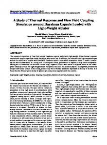
List of Figures 2.1. Definition of the coordinate system and the variables of the shallow water equations. . . . . . . . . . . . . . . . . . . . . . . . . . . . . . . . . . . . . .

16

3.1. Cells with centers P and N , separated by face f . . . . . . . . . . . . . . . . 3.2. Boundary cell with center P and boundary face with center b. . . . . . . . .

24 30

4.1. Initial conditions of the lake at rest. . . . . . . . . . . . . . . . . . . . . . . . 4.2. Solutions of the lake at rest at different times t: Without the mixed centralupwind scheme and with the mixed central-upwind scheme. . . . . . . . . . . 4.3. Elevation map of the Glasgow benchmark test. . . . . . . . . . . . . . . . . . 4.4. Comparison of shallowFoam with other 2D shallow water solvers: Water level time series and velocity time series. . . . . . . . . . . . . . . . . . . . . . . . 4.5. Normalized profiles of u, k and ω for parameter combinations C1 and C2. . . 4.6. Normalized profiles of u, k and ω for parameter combinations C3 and C4. . .

42

5.1. 5.2. 5.3. 5.4.

42 44 45 50 51

Overlapping and non-overlapping subdomains. . . . . . . . . . . . . . . . . . Meshes at the interface: Side view and top view. . . . . . . . . . . . . . . . . Example of a global mesh setup. . . . . . . . . . . . . . . . . . . . . . . . . . Characteristics in the vicinity of a boundary: Subcritical conditions and supercritical conditions. . . . . . . . . . . . . . . . . . . . . . . . . . . . . . . . 5.5. Transfer of variables for all four combinations of flow direction and flow condition. . . . . . . . . . . . . . . . . . . . . . . . . . . . . . . . . . . . . . . . 5.6. Side view on the cells at the interface with the local bottom elevations, the local flow depths, and the horizontal distances between the cell centers and the interface. . . . . . . . . . . . . . . . . . . . . . . . . . . . . . . . . . . . 5.7. Calculation of indicator function α1 for a face on Γ3D . . . . . . . . . . . . . . 5.8. Flowchart of the coupled simulation. . . . . . . . . . . . . . . . . . . . . . . 5.9. Interfield and intrafield time-stepping diagram of the staggered solution procedure. . . . . . . . . . . . . . . . . . . . . . . . . . . . . . . . . . . . . . . . 5.10. Directory trees for three types of simulations: 2D, 3D and coupled. . . . . . 5.11. Excerpts of the boundary files of corresponding 2D and 3D patches. . . . . . 5.12. Examples for the definition of a scalar and a vector boundary condition. . . . 5.13. Excerpt from the top level source code file. . . . . . . . . . . . . . . . . . . . 5.14. Example for the geometry mapping algorithm. . . . . . . . . . . . . . . . . .

54 57 58

6.1. 6.2. 6.3. 6.4.

84 87 90 91

Basic geometrical setup of all plane flow test cases. . . . . . . . . . . . . . Initial Gauss wave from eq. (6.1) with µ = 30 m and σ = 2.5 m. . . . . . . 2D solutions of the upstream travelling waves with different wave height H. 3D solutions of the upstream travelling waves with different wave height H.

. . . .

59 64

65 67 73 73 76 77 78 80 80

XI

XII

List of Figures 6.5. 2D, 3D and 2D→3D solutions of upstream travelling waves with H = 0.2 m. 6.6. 2D, 3D and 3D→2D solutions of upstream travelling waves with H = 0.2 m. 6.7. Details of the 2D→3D solution and the 3D→2D solution of the upstream travelling waves with wave height H = 0.2 m. . . . . . . . . . . . . . . . . . 6.8. Details of the upstream travelling wave with different CFL numbers. . . . . . 6.9. Volume balance in the region 0 < x < 35 m for all four setups. . . . . . . . . 6.10. 2D, 3D and 2D→3D solutions of the two downstream travelling waves with H = 0.1 m under supercritical conditions. . . . . . . . . . . . . . . . . . . . 6.11. 2D, 3D and 3D→2D solutions of the two downstream travelling waves with H = 0.1 m under supercritical conditions. . . . . . . . . . . . . . . . . . . . 6.12. Schematic of the force-time history with four distinct segments. . . . . . . . 6.13. Top view of the meshes with the block at the center. . . . . . . . . . . . . . 6.14. Evolution of the flow depth h for the coupled case at different times t. . . . . 6.15. Detail of the splash in front of the block. . . . . . . . . . . . . . . . . . . . . 6.16. Streamwise profiles of flow depth h in the symmetry plane. . . . . . . . . . . 6.17. Formation of the upstream travelling shock waves in front of the block. . . . 6.18. Streamwise profiles of flow depth h at the lateral coupling interface. . . . . . 6.19. Drag force Fd and drag coefficient Cd over time for 2D, 3D and coupled case. 6.20. Flow depth h of the full 3D cases with meshes M1 and M05 at time t = 16 s. 6.21. Drag force Fd and drag coefficient Cd over time for the 3D case with meshes M2, M1 and M05. . . . . . . . . . . . . . . . . . . . . . . . . . . . . . . . . . 6.22. Influence of the interface compression coefficient Cα on the drag force Fd . . . 6.23. Blocking of the upstream travelling hydraulic jump at the 2D/3D interface. . A.1. A.2. A.3. A.4.

2D, 2D, 2D, 2D,

3D 3D 3D 3D

and and and and

2D→3D 2D→3D 3D→2D 3D→2D

solutions solutions solutions solutions

of of of of

upstream upstream upstream upstream

travelling travelling travelling travelling

waves waves waves waves

with with with with

H H H H

= 0.1 = 0.3 = 0.1 = 0.3

m. m. m. m.

93 94 95 98 98 101 103 107 107 111 112 113 114 115 116 117 118 120 121 141 142 143 144

Notation Roman Letters A Axy a b CFL C0 CD Cα C− C+ c cν d F F FC FD FD fx g H H H H HU h h0 hdry hdry,2 hclip hinit

= = = = = = = = = = = = = = = = = = = = = = = = = = = = = = =

amplitude of Gauss curve (m) 2 horizontal cross-sectional area of Ωloc 3D (m ) implicit discretization coefficient width of a structure (m) Courant-Friedrich-Lewy number (–) characteristic of the SWE (m s−1 ) drag coefficient (–) compression coefficient of the VOF method (–) receding characteristic of the SWE (m s−1 ) advancing characteristic of the SWE (m s−1 ) wave celerity (m s−1 ) constant of eddy viscosity model (–) vector between two adjacent finite volume cells (m) face flux (m3 s−1 ) Froude number (–) discretized convection term drag force (kg m s−2 ) discretized diffusion term interpolation coefficient (–) gravitational acceleration vector (m s−2 ) typical horizontal length scale (m) wave height (m) transport part in the semi-discretized momentum equation flow depth h in shallowFoam (m) specific discharge q in shallowFoam (m2 s−1 ) flowdepth (m) fluctuating flowdepth (m) auxiliary flowdepth (m) auxiliary flowdepth (m) auxiliary flowdepth (m) initial flowdepth (m)

XIII

XIV hint IS k ks kSt kst L n n n∗ nut p pa pd q qin qout S S S S SE SI SI,τ Sij Sφ t U UR U ui ui ur u∗ V V˙ IF V init W

Notation = = = = = = = = = = = = = = = = = = = = = = = = = = = = = = = = = = = = = =

internal flowdepth (m) bottom slope (–) turbulent kinetic energy (m2 s−2 ) equivalent sand grain roughness (m) Strickler’s coefficient (m1/3 s−1 ) Strickler’s coefficient kSt in shallowFoam (m1/3 s−1 ) typical vertical length scale (m) Manning’s coefficient (s m−1/3 ) normal vector (–) normal vector of the interface in the VOF method (–) turbulent viscosity νt in shallowFoam (m2 s−1 ) pressure (kg m−1 s−2 ) atmospheric pressure (kg m−1 s−2 ) modified pressure of the interFoam solver (kg m−1 s−2 ) specific discharge (m2 s−1 ) specific inflow (m2 s−1 ) specific outflow (m2 s−1 ) closed surface around finite volume cell (m2 ) discretized source term face area vector (m2 ) bottom elevation zb in shallowFoam (m) explicit part of source term Sφ implicit part of source term Sφ implicit source term due to bottom friction (s−1 ) fluctuating rate of strain tensor (s−1 ) source term in the generic transport equation time (s) typical horizontal velocity scale (m s−1 ) Ursell number (–) velocity vector (m s−1 ) ith component of velocity (m s−1 ) ith component of depth averaged velocity (m s−1 ) compression velocity of Volume-of-Fluid method (m s−1 ) friction velocity (m s−1 ) volume (m3 ) volume production term of the coupling interface (m3 m−1 s−1 ) initial volume of plane waves (m3 m−1 ) typical vertical velocity scale (m s−1 )

Notation x zb zf zfrel zw

XV = = = = =

position vector (m) bottom level (m) absolute level of face center (m) level of face center relative to bottom level (m) water level (m)

Greek Letters α1 β Γ Γ2D Γ3D ∆2D ∆3D ∆t ∆x, ∆y, ∆z ∆zf η κ λ µ µ µt ν νa νt νw ρ ρa ρw σ τbi τij φ Ωloc 2D Ωloc 3D ω

= = = = = = = = = = = = = = = = = = = = = = = = = = = = = = =

indicator function of Volume-of-Fluid method (–) mass conservation corrector (–) diffusion coefficient (m2 s−1 ) 2D side of the coupling boundary 3D side of the coupling boundary horizontal distance between 2D cell centers and coupling boundary (m) horizontal distance between 3D cell centers and coupling boundary (m) time step width (s) grid resolution in x-, y- and z-direction, respectively (m) height of a boundary face (m) turbulent dissipation (m2 s−3 ) Kolmogorov length scale (m) von-Karman’s constant (–) wave length (m) mean of Gauss curve (m) molecular dynamic viscosity (kg m−1 s−1 ) turbulent dynamic viscosity (kg m−1 s−1 ) molecular kinematic viscosity (m2 s−1 ) molecular kinematic viscosity of air (m2 s−1 ) turbulent kinematic viscosity (m2 s−1 ) molecular kinematic viscosity of water (m2 s−1 ) density (kg m−3 ) density of air (kg m−3 ) density of water (kg m−3 ) standard deviation of Gauss curve (m) ith component of bed stress (kg m−1 s−2 ) lateral stresses in shallow water equations (kg m−1 s−2 ) generic quantity (–) 2D cell next to the coupling boundary column of stacked 3D cells next to the coupling boundary specific turbulent dissipation (s−1 )

XVI

Notation

Sub- and Superscripts ·a ·b ·b ·f ·N ·n ·P ·s ·w · 2D · 3D ·n · n+1

= = = = = = = = = = = = =

air bottom value at a boundary face center value at a face center value at a neighboring cell center vector component normal to the coupling boundary value at a cell center vector component tangential to the coupling boundary water value in the 2D region value in the 3D region value at old time level n value at new time level n + 1

Mathematical Operators ∇ · h·i ·0 · e·

= = = = = =

Nabla operator dot product ensemble average of Reynolds-decomposed quantity fluctuating part of Reynolds-decomposed quantity mean of depth-averaged quantity fluctuating part of depth-averaged quantity

1. Introduction Modern human society constantly strives for an economic use of resources like money, labor or time. Under the premise of an accurate pricing, even the economic use of natural resources would be something to strive for. What holds for society, equally holds for the realm of engineering, which is also in a constant strive for the economic use of resources. This can be achieved only if the problem at hand is thoroughly understood, with all its relevant parameters and the interaction between those parameters. The three major tools to obtain a solid understanding are theory, experiment and simulation. Theory and experiment both are well established methods, with a lot of advantages, but also with a number of disadvantages: Theory offers the deepest insight into a problem, but it is often limited to rather simple systems; complex systems with possible non-linear interactions usually are beyond the capabilities of theoretical approaches. Experiments are able to represent such complex, non-linear systems, however, they often are expensive in terms of money and/or time (especially in case of parameter studies). In addition, it can be difficult to measure the relevant quantities, or scaling effects can make it difficult to capture all relevant parameters. Numerical simulations can deliver insights, where theoretical or experimental approaches are not applicable. Especially their predictive capabilities for complex, non-linear systems make them an invaluable tool in literally all fields of engineering. However, also numerical simulations come at a cost: It costs money to provide the required computer power, it costs labor to set the simulations up and to evaluate the results, and it costs time to obtain the results, especially for larger systems with complex physics. Not to mention the cost to validate the results, or the potential cost of invalid results. In this thesis numerical simulations will be applied to environmental free surface flows. Environmental flows have been one of the first fields of application for computational fluid dynamics (CFD), starting with numerical weather prediction in the 1950’s (Charney, Fjörtoft, & Von Neumann, 1950). Since then, a wide range of free surface flows have been investigated by means of numerical simulations, and many of the developments in this field would not have been possible without them. However, due to the complexity of the phenomenon, further research is required.

1.1. Motivation Environmental free surface flows are probably one of the most complex fields of engineering applications. They typically • are governed by a wide range of spatial scales (from tidal currents and catchments to hydraulic structures down to the turbulent length scales),

1

2

1.1. Motivation • cover irregular, often unsteady spatial domains (main channel, floodplains, erosion, sediment transport), • have unsteady or even unknown boundary conditions (flood, drought, surface roughness, wet/dry interface, coast line, subsurface flow), • interact with the built environment (dams, dikes, groynes, weirs, bridge piers, breakwaters), • interact with the ecosystem, like vegetation, which is subject to (seasonal) change, • include secondary flow structures, that can be difficult to quantify, • can be subject to a number of driving forces (gravity, wind, atmospheric pressure gradients, Coriolis force, tidal forces), • will be subject to long term climatic changes (frequency of flash floods, increasing intensity of general precipitation (Min, Zhang, Zwiers, & Hegerl, 2011), all of them due to an increasing amount of energy in the atmosphere), • can contain pollutants (from point sources or diffusive sources, e.g. salination, nitrification, micro plastics) as well as sediment or driftwood.

In addition to the influence of the single aspects, every aspect usually interacts with a variety of other aspects. Including all of these aspects into one simulation would render this simulation infeasible, due to the large range of spatial and time scales, unknown physics and unknown boundary conditions. In general all environmental free surface flows are three-dimensional, and it would be possible to model them with a set of 3D equations – Navier-Stokes or Reynolds-Averaged NavierStokes (RANS) equations. However, for many applications this would be computationally very expensive, if not impossible. Hence, following the economic principle from the beginning of this chapter, it is desirable to reduce the complexity of the problem wherever possible. A discussion of all the possible simplifications, and their potential consequences, would be out of the scope of this work. Instead the focus will be put on the first point on the list, the spatial scales. One of the most common ways to reduce the spatial complexity of an environmental free surface flow is a spatial averaging over its vertical dimension, hence reducing the spatial dimensions of the problem from three to two. The solution of the resulting 2D shallow water equations (SWE) is far less expensive than the solution of the original 3D RANS equations. The 2D SWE are one of the most common tools in hydraulic engineering, they are routinely used for tasks like flood modelling on the catchment scale, and they usually do not require calibration. A further simplification can be obtained by horizontal averaging of the SWE, yielding the 1D St.-Venant equations (SVE). The SVE also are a common tool in hydraulic engineering, for tasks like large-scale conveyance modelling. However, 1D models usually require proper calibration, and hence are not suited for the prediction of extreme events. In the following, the focus will be on the 3D RANS equations and the 2D SWE. Despite their advantages in terms of efficiency, the SWE often are valid only in parts of the domain; in other parts of the domain the full 3D RANS equations would be required. The distinction between shallow flows, where the SWE are valid, and non-shallow flows, where the RANS equations are required, will be discussed in section 1.2.1. The limitations of the SWE, i.e. which phenomena can not be modelled via the SWE, will be discussed in section 1.2.2.

1. Introduction

3

As will be shown in section 1.2, a flow usually is not completely shallow or completely nonshallow. Instead, it often comprises of both: Regions with shallow, 2D flow characteristics, and regions with non-shallow, 3D flow characteristics. Therefore, a coupling between the two sets of equations could deliver both: The efficiency of the SWE – wherever possible, and the accuracy of the RANS equations – wherever required. A discussion on coupling methods in hydraulics will be provided in section 1.3. Another aspect that governs the complexity of a flow problem are the turbulent scales. Nearly all environmental free surface flows are turbulent, and in most cases the resolution of the turbulent scales would go far beyond the capabilities of any present computer system. Therefore the question arises how to model the turbulent scales of environmental free surface flows. This point will be discussed in section 1.4.

1.2. Shallow and Non-Shallow Flows As mentioned above, it is often desirable to reduce the spatial complexity of an environmental free surface flow. In the case of the 2D SWE this is achieved via a spatial averaging over the vertical dimension. In section 1.2.1 it will be discussed where exactly such a simplification is feasible, and in section 1.2.2 the consequences of the resulting loss of information, which comes with the reduced spatial dimensions, will be detailed.

1.2.1. Distinction Shallow – Non-Shallow The decisive parameter for the distinction between shallow and non-shallow flows is the ratio between a typical vertical length scale H, and a typical horizontal length scale L. But what constitutes a typical scale? This can not be answered in a general sense, it always depends on the local flow conditions, and a flow can be both, shallow and non-shallow, at the same time. Typical vertical length scales could be the flow depth, the amplitude of a wave, the height of a roughness element, the vertical extent of hydraulic structures like dikes or groynes, the variation of the bottom level, or any other vertical length scale that affects the flow conditions. Typical horizontal length scales could be the width of a river, a wave length, the horizontal extent of structures like dikes or groynes, the width of a bridge pier, the distance over which the bottom topography varies or the width of a roughness element. The basic assumption of the shallow water theory is that the ratio between the decisive vertical length scale and the decisive horizontal length scale is very small: H/L 1 (the question of what constitutes a decisive length scale will be discussed later). From linear wave theory, which is not based on the shallow-water assumption from the outset, Le Méhauté (1976, p. 210) gives an upper limit of H/L = 0.05 for very shallow water waves, and an upper limit of H/L = 0.1 for shallow water waves. It becomes obvious that there is not one fixed limit for the SWE to be valid, but that one can rather expect an increasing error, the

4

1.2. Shallow and Non-Shallow Flows

bigger the ratio between horizontal and vertical length scale becomes. From the assumption of shallowness one can derive (see section 2.2.1) that the vertical velocity component w must be much smaller than the horizontal velocity components u and v, and thus can be neglected. The vertical momentum equation of the Navier-Stokes equations then reduces to the hydrostatic pressure distribution, and the remaining variables are the horizontal velocities, thus yielding the reduction from three to two dimensions. But which of the length scales are the decisive ones in a given problem? This depends on the point of view: Looking for instance at a wide river reach, typically the width of the river and the flow depth are the decisive horizontal and vertical length scales, respectively, and the flow could be considered as shallow. However, if one is interested in the local flow field around a bridge pier in the same river reach, the decisive horizontal length scale would now be the width of that bridge pier. Consequently, with the flow depth typically being of the same order as the width of the bridge pier, the flow there could not be considered as shallow anymore. So the flow in the river reach is shallow and non-shallow at the same time. A similar line of argument can for instance be made for a wave with a small wave length on the surface of the river, or for the flow field in the vicinity of a bottom step. However, modelling the river reach and its bridge pier exclusively with the shallow water equations could still yield accurate results for the major part of the flow field, as long as the influence of the error, which is made at the bridge pier, does not become too big. The reasons and the consequences of such errors will be discussed in the next section.

1.2.2. Limitations of the Shallow Water Equations The limitations of the SWE are the result of the simplifications that they are based on. The two basic simplifications are the neglect of the vertical velocity component (that directly results in the hydrostatic pressure distribution), and the depth-averaging of the horizontal velocities. The consequences of these simplifications will be discussed in the following. Neglecting the vertical velocity component results in a suppression of secondary flow structures, especially of large-scale rotating structures with the axis of rotation in streamwise direction. The lack of such structures directly impacts the lateral transfer of momentum, mass and other quantities. Lateral momentum transfer can act as both a driving force or a resisting force (Vreugdenhil, 1994), such that it is hard to predict the consequences of its absence. Lateral mass transfer plays a role in processes like the tilting of the water surface in river bends, such that its absence can impact the prediction of the water level. The lateral transport of scalars influences the mixing of quantities like heat or pollutants, such that the lack of this term can inhibit the correct prediction of the dispersion characteristics of such quantities. An exact derivation of the lateral transport term and some modelling approaches will be provided in section 2.2. The depth-averaging of the vertical velocity profiles results in the loss of information about the velocity gradient, such that the bottom friction can not be obtained directly anymore,

1. Introduction

5

instead it has to be modelled. Independent of the chosen model, this model will always be inferior to the 3D-based computation of the bottom friction, and hence a potential source of error. The bottom friction is, besides the gravity term, the major source term in the SWE, so its modelling has a direct impact on the solution. The bottom friction also governs processes like sediment transport, scouring and erosion. The modelling of such processes is already a challenge in 3D models, so it becomes increasingly difficult in 2D, and usually requires proper calibration. Furthermore the absence of a vertical velocity profile also has an impact on the scalar dispersion characteristics of the flow, hence making it more difficult to correctly predict the distribution of sediment or pollutants. Waves with short wave lengths which can occur at the surface of a flow that is considered as shallow (see above), induce a vertical velocity component. Due to the absence of this component, the SWE are not able to represent such waves. In order to be able to include fairly long waves, the Boussinesq approximation can be employed that makes use of a Taylor series expansion to express the vertical component in terms of the horizontal components. Dingemans (2000) gives an upper limit of H/L = 1/7 for the applicability of the Boussinesq approximation. The original SWE can also not be applied where the bulk flow has a significant vertical velocity component, e.g. in steep alpine rivers or on spillways of dams. In such cases the flow is not hydrostatic, and a non-hydrostatic extension of the SWE could be applied. In such extensions the vertical accelerations in the vertical momentum equation are taken into account, such that this equation does not simplify to the hydrostatic pressure distribution (see section 2.2). Examples for this type of equations are the Serre-type equations (Dias & Milewski, 2010). One further implicit assumption in the derivation of the SWE is the existence of a free surface. Consequently, it is not possible to use the SWE to model flows without a free surface, like they appear in filled pipes or at hydraulic structures like sluice gates. All these errors and limitations are inherent to the standard SWE, and do not appear in the 3D RANS equations. With a coupling between the SWE and the RANS equations, it would be possible to model those parts of the domain, where the above mentioned phenomena occur, by means of the RANS equations, and the remaining parts of the domain with the SWE. Coupling approaches in the field of hydraulics will be discussed in the following section.

1.3. Coupling Methods As it was shown in the previous section, a free surface flow often can be considered as shallow in some parts of the domain, and as non-shallow in other parts. Therefore a simulation environment, where the two solutions are coupled would be able to combine the strengths of both approaches: The spatial resolution of the 3D RANS solver, with the efficiency of the 2D SWE solver. The coupling between different models is common practice in many fields of applications, like fluid-structure interaction or multi-scale methods. Also in hydraulics

6

1.3. Coupling Methods

the coupling between different models has been applied in a number of ways, some of which will be described in the following. One of the most common approaches is the modeling of hydraulic structures in a 2D SWE solver by means of so-called 1D links. The flow in hydraulic structures like weirs or sluice gates is often difficult or impossible to capture via the SWE, due to the inherent 3D flow characteristics in many of those structures. However, there often exist 1D formulas, usually derived from the Bernoulli equation, that give a stage-discharge relationship for such hydraulic structures. These can be included via a 1D link into the 2D SWE, which usually couples the flow depth on the upstream side with the discharge on the downstream side of the structure, but possibly also taking into account more variables. One of the drawbacks of this method is the fact that the 2D flow has to be averaged horizontally, in order to obtain the 1D variables, and therefore no horizontal variability can be take into account. This can be partially prevented by a zonal approach, where the 2D flow is averaged in a piecewise manner. However, this approach is still limited to flow situations for which such 1D formulas exist, and it is not generally applicable. Also the coupling of the 2D SWE with larger 1D subsystems is common practice in hydraulics. Three approaches can be distinguished: Longitudinal coupling, lateral coupling and coupling via superposition: • In longitudinal coupling the 1D and the 2D regions are solved independently from each other, and they are coupled via inflow/outflow boundary conditions. Chen, Wang, Liu, and Zhu (2012) ensured conservation of mass at the 1D/2D interface, and Bladé et al. (2012) additionally ensured conservation of momentum. This approach is well-suited for the modelling of river-lake or river-estuary systems. • In lateral coupling the flow in a channel, or a network of channels, is simulated in 1D, and the 2D domain is located laterally to the 1D channels. The 1D and the 2D domain have been coupled via Manning’s equation by Kuiry, Sen, and Bates (2010), or via a weir formula by Ahmadian, Falconer, and Wicks (2015). • In coupling via superposition a 1D network of channels is (partially) superposed by a 2D domain. D’Alpaos and Defina (2007) used the continuity equation to couple the 1D and the 2D domain. Gejadze and Monnier (2007) used a source term for the information transfer from 2D to 1D, and inflow/outflow boundary conditions for the information transfer from 1D to 2D. In the two latter coupling approaches, lateral and via superposition, the 2D domains remain inactive, as long as the 1D flow does not overtop its embankments. Consequently, the major application of such approaches is the river-floodplain modelling. Two of the coupling approaches, longitudinal and via superposition, have been combined in one single model by Viero, D’Alpaos, Carniello, and Defina (2013), who modeled a levee breach by means of longitudinal coupling, and integrated this in the laterally coupled model of D’Alpaos and Defina (2007). Another approach is the coupling of the 2D SWE with 1D pipe models, to account for the contribution of the sewage system, for instance in urban flood scenarios. Leandro, Chen, Djordjević, and Savić (2009) used a coupled sewer/surface model to calibrate a 1D/1D hy-

1. Introduction

7

drological model. Adeogun, Daramola, and Pathirana (2015) conducted a sensitivity analysis of the mesh resolution, of the resolution of the digital elevation model and of the surface roughness for a coupled sewer/surface model. Further common coupling approaches are the coupling between 2D surface and 3D subsurface models, such that the interaction between the surface and the groundwater flow can be taken into account, or the coupling between a hydraulic model and a general hydrological model, where the hydrological model can deliver realistic boundary conditions for complete catchments. Less common so far is the coupling between 2D and 3D surface flow models, publications on this topic are rather scarce. Qi and Hou (2004) coupled a 2D Boussinesq model with a 3D RANS model, and used the Volume-of-Fluid method of Hirt and Nichols (1981) for the free surface tracking in the 3D region. The information transfer between the two models was implemented via an overlap region, where they imposed a direct matching between water level and velocities. The vertical velocity profiles have been obtained from the solution of the Boussinesq equations. They were able to reduce the computational effort by 90 % with respect to a full 3D model, and achieved a good agreement with the velocity profiles of the full 3D model. Unfortunately the description of the solver is incomplete, and no further validation data has been provided. A one-way coupling between the SWE and the RANS equations has been implemented by Kilanehei, Naeeni, and Namin (2011), who used the results of a 2D simulation of a river reach as initial and boundary conditions of a 3D RANS solver. The advantages of such an approach are the realistic boundary conditions and the fast convergence that can be expected for the 3D solver. However, only steady-state scenarios can be captured with this approach, and the possible feedback effects from 3D to 2D, like backwater for instance, can not be taken into account. Gerstner, Belzner, and Thorenz (2014) used an iterative coupling between the 2D SWE solver Hydro AS-2D, and the 3D free surface RANS solver interFoam (the one that is also used in this work for the 3D region), to incorporate backwater effects. They assessed how the flood routing of a 100-year flood event was influenced by a failing weir gate. In 2D they modelled the weir via a weir formula with an overflow coefficient µ, and in 3D the weir was modelled with its complete geometry. They used an iterative procedure to couple the two models: The 2D results were used as boundary conditions of the 3D model, and the results of the 3D model were incorporated into the 2D model via the overflow coefficient µ. With this procedure they obtained satisfactory results. However, this approach requires a number of 2D and 3D simulations, until the deviation between the two models is acceptable, and also here only steady state conditions can be investigated. The results of Kilanehei et al. (2011) and of Gerstner et al. (2014) emphasize the benefits of a direct, bi-directional coupling between a 2D SWE and a 3D RANS solver: The interaction between the two solvers can be taken into account directly, thus enabling the simulation of unsteady phenomena, and avoiding the need for computationally expensive

8

1.5. Contribution of This Work

multiple simulations of any of the regions.

1.4. Treatment of Turbulence Nearly all environmental free surface flows are essentially three-dimensional (3D) and turbulent, with spatial extension and velocities in all three directions. The governing spatial scales range from the integral length scale L, which is governed by the outer dimensions of the flow, down to the Kolmogorov length scale η. The Kolmogorov length scale represents the size of the smallest turbulent structures, with η in hydraulics usually being in the range of 0.01 – 0.1 mm.1 The basic set of equations to describe any kind of 3D flow, laminar or turbulent, are the Navier-Stokes equations (NSE). In numerical simulations, the NSE form the basis of the Direct Numerical Simulation (DNS), where all relevant spatial and temporal scales, from the integral down to the turbulent scales, are resolved. For a river reach with dimensions 1×1×10 m, and a Kolmogorov scale of 0.1 mm, the required resolution would be = 1 · 1013 , hence rendering the use of DNS for real world applications impossible. N = 1×1×10 0.00013 One way to reduce the computational effort is the use of the Large Eddy Simulation (LES) method, where only the large turbulent structures are simulated directly. The smaller turbulent scales are filtered (usually by the size of the computational grid), and their dissipative influence is modelled via a turbulence model. LES has been applied successfully to a number of applications in hydraulics (Rodi, Constantinescu, & Stoesser, 2013), but it is still relatively expensive, and therefore not widely spread. The most common method in hydraulics is the numerical solution of the Reynolds-Averaged Navier-Stokes (RANS) equations: Here the NSE are time- or ensemble-averaged, resulting in the RANS equations that contain an additional term, the Reynolds stresses. In the so-called eddy viscosity models, the Reynolds stresses are modeled in analogy to the molecular viscous stresses, with a turbulent viscosity νt . The major task of the RANS models is then to model νt via the mean flow variables. There exists an abundance of approaches for this task, some of which will be discussed in section 2.1.4. The disadvantage of RANS with respect to LES is the fact that in the RANS approach all turbulent scales are modelled, whereas in the LES approach the larger, energy containing structures are simulated directly. This can become problematic since the isotropy of turbulence increases towards the smaller scales, meaning that the larger scales are rather non-isotropic, making it more difficult to model them appropriately. In shear layers for instance, with their strong anisotropic large scale turbulence, RANS models are usually not able to provide accurate results without calibration. However, for attached flows, which are the most common in the field of hydraulics, RANS models are able to provide reliable results without the need for calibration.

1.5. Contribution of This Work In this work the two-way coupling between a 2D shallow water solver and a 3D ReynoldsAveraged Navier-Stokes solver with free surface will be presented. With the coupled solver, 1

With kinematic viscosity ν = 1 · 10−6 m2 /s, a typical length scale l = 1 m and a typical velocity u = 1 m/s, the Kolmogorov scale is η = (ν 3 l/u3 )1/4 = 0.0316 mm.

1. Introduction

9

it is possible to combine the strengths of both approaches – the efficiency of the 2D solver and the accuracy of the 3D solver. The coupled solver can be utilized in essentially two ways: • For the detailed investigation of a 3D flow phenomenon, the 2D solver can be used to deliver realistic boundary conditions to the 3D solver. The size of the 3D domain can be restricted to the actual region of the 3D flow, there is no more need to simulate the inflow or the outflow conditions with the expensive 3D solver, hence resulting in an increased efficiency of the simulation. • In large scale 2D simulations like flood scenarios, the 3D solver can be used for the accurate modelling of local 3D phenomena. The results of the 2D solver are no longer corrupted by the 2D solver’s poor representation of the 3D phenomena, thus yielding a higher accuracy of the results. The coupled solver has been implemented with its application to riverine flows in mind – however, it should be applicable as well to a wide range of other environmental free surface flows. The two solvers that have been coupled in this work, shallowFoam and interFoam, are both R publicly available as Open Source software in the OpenFOAM framework2 (OpenCFD Ltd, 2009). interFoam is part of the original distribution of OpenFOAM, and shallowFoam has been developed at Technical University of Munich. Also the coupled solver will be made publicly available under the name shallowInterFoam on the gitHub platform,3 thus allowing anyone to use and modify the solver to their own needs. The description that is given in this thesis is supposed to be sufficiently detailed to understand the source code. The application of the solver, without any programming requirements, will be described in detail in section 5.7. Also a number of example cases will be provided on gitHub.

1.6. Outline The outline of this work is the following: The Reynolds-Averaged Navier-Stokes equations for non-shallow 3D flow will be given in section 2.1, together with a model for free surface flow and the turbulence closure. In section 2.2 the 2D shallow water equations will be derived from the 3D equations, and models for bottom friction and turbulence will be provided. The numerical solution of the 2D and the 3D equations will be described in chapter 3: First the basics of the Finite Volume Method, which is used in this work, will be provided in section 3.1, with a special focus on the numerical implementation of boundary conditions. Then the specifics of the 3D RANS solver will be introduced in section 3.2, and the specifics of the 2D SWE solver will be given in section 3.3. Both of these sections include a general description of the physical boundary conditions that are commonly used in the respective solver. In chapter 4 three sets of preliminary test cases will be shown: First a validation of a mixed central-upwind differencing scheme, which has been implemented to stabilize the 2D solution at the wet/dry interface (4.1). Then the 2D solver will be validated by means of a comparison to a wide variety of other 2D SWE solvers (4.2). At the end of this chapter 2

OpenFOAM is a registered trade mark of OpenCFD Limited, producer and distributor of the OpenFOAM software via wwww.openfoam.com. 3 https://github.com

10

1.6. Outline

the results of a set of numerical experiments with the 3D solver will be shown, which will be used in the implementation of the coupling algorithm to provide realistic vertical inflow profiles for the velocity and the turbulence variables (4.3). The coupling algorithm will be described in chapter 5, including some background on coupling methods (5.1), basics of domain decomposition methods (5.2), the mesh structure of a coupled simulation (5.3), the number and the type of boundary conditions that are required for the coupling of SWE and RANS equations (5.4), the calculation of the boundary conditions that constitute the coupling (5.5), the solution procedure of the coupled solver (5.6), the setup of a coupled simulation (5.7) and some technical aspects of the implementation (5.8). The coupling method will be validated on two sets of test cases in chapter 6: In section 6.1 the results of a set of plane wave test cases will be presented, where the influence of the coupling interface on the wave transport will be examined. The coupled results will be compared to the results of pure 2D and pure 3D simulations. In this set of test cases also the mass conservation properties of the coupled solver will be tested, as well as the stability of the coupling with respect to the CFL limit. In section 6.2 the coupling method will be employed to simulate the impact of a hydraulic bore on a structure. The resulting flow depths, drag forces and drag coefficients will be evaluated and compared to the results of a pure 2D and a pure 3D simulation. Furthermore the influence of mesh refinement and of a compression parameter of the 3D free surface model will be examined. An open issue of the coupling method with respect to an upstream travelling hydraulic jump will be discussed, and the influence of the coupling on the overall runtime will be investigated. In chapter 7 a summary and conclusion of the present work will be provided, and some possible directions for future research will be outlined.

2. Theory In this chapter the theoretical foundation of the present work will be given. Section 2.1 describes the theoretical concepts that are used for general, non-shallow flows: The threedimensional Navier-Stokes equations, the Reynolds-Averaged Navier-Stokes equations, the two-phase methodology and the turbulence closure. The theory of shallow flows will be covered in section 2.2, where the simplification of the 3D equations to the two-dimensional shallow water equations will be described. Furthermore modelling of bottom friction and turbulence will be specified, and finally some of the effects that are not covered in the 2D approach will be pointed out.

2.1. Equations for 3D Flows In this section the full Navier-Stokes equations for an incompressible Newtonian fluid will be given. Then the Reynolds decomposition and the resulting Reynolds-Averaged NavierStokes equations will be described, followed by a brief overview of existing turbulence models. Finally, a detailed description of the k-ω-SST model used in this work will be given.

2.1.1. Navier-Stokes Equations Based on the continuum hypothesis, every incompressible Newtonian flow can mathematically be described by the Navier-Stokes equations, with conservation of mass ∂ui =0 ∂xi

(2.1)

and conservation of momentum ∂ui ∂ui 1 ∂p ∂ ∂ui ∂uj + uj =− + ν + + gi ∂t ∂xj ρ ∂xi ∂xj ∂xj ∂xi

(2.2)

with the instantaneous velocities ui , density ρ, pressure p, kinematic viscosity ν, and gravity gi , assuming that the latter is the only relevant body force.

2.1.2. Reynolds-Averaged Navier-Stokes Equations The relevant spatial scales of the full Navier-Stokes equations reach down to the Kolmogorov scale η, which in hydraulics has a typical order of magnitude of 0.01 – 0.1 mm (see section 1.4 for an exemplary computation of η). For field applications the resolution of such a small scale is computationally not feasible. By means of the Reynolds decomposition the small scales

11

12

2.1. Equations for 3D Flows

of a flow field can be described statistically. The resulting Reynolds-Averaged Navier-Stokes equations are a set of mean flow equations with a fluctuating part which needs to be modelled. Application of the Reynolds decomposition φ = hφi + φ0

(2.3)

to eqs. (2.1) and (2.2) – with the ensemble-average hφi of a quantity φ and the fluctuating part φ0 of this quantity – yields the Reynolds-Averaged Navier-Stokes (RANS) equations: ∂hui i =0 ∂xi

(2.4)

0 0 ∂hui i 1 ∂hpi ∂ ∂hui i ∂huj i ∂hui i + huj i =− + ν + − ui uj + gi (2.5) ∂t ∂xj ρ ∂xi ∂xj ∂xj ∂xi

with the Reynolds stress tensor u0i u0j . Eq. (2.5) contains six independent unknowns of the symmetric Reynolds stress tensor, thus leaving this equation unclosed. Based on the eddy viscosity hypothesis, the Reynolds stresses can be related to the rate-of-strain of the mean flow via a turbulent viscosity νt , leading to a closed form of the Reynolds-Averaged Navier-Stokes equations 1 ∂p ∂ ∂ui ∂ui ∂ui ∂uj =− + + + uj (ν + νt ) + gi . (2.6) ∂t ∂xj ρ ∂xi ∂xj ∂xj ∂xi Here the ensemble-averaging operator h · i has been dropped, which will be the convention from now on. This means ui represents the ensemble-averaged flow vector. Modelling of the turbulent viscosity will be described in sections 2.1.4 and 2.1.5.

2.1.3. The Volume-of-Fluid Method In the present range of applications, the flow is in general a free-surface flow. The free surface needs to be modelled, which can be done by a number of different approaches that can be classified in three categories: Surface tracking, moving mesh and volume tracking methods (see Rusche (2002, p. 38ff.) for a detailed description and further references to each of these methods). The method that is used here is the Volume-of-Fluid method of Hirt and Nichols (1981), which is a volume tracking method. This method employs a continuous indicator function α1 , which indicates the volume fraction of the two fluids A and B at a specific point in space and time:  in fluid A,  0 in fluid B, α1 (x, t) = 1 (2.7)   0 < α1 < 1 in the continuous interface between A and B.

2. Theory

13

The transport equation for α1 is ∂α1 ∂α1 ∂α1 (1 − α1 ) + uj + urj = 0, ∂t ∂xj ∂xj

(2.8)

where the third term is an artificial compression term that has been introduced by Rusche (2002, p. 152ff.). Due to the term α1 (1−α1 ), this compression term is only active in the region of the interface, where it counteracts the diffusion of α1 and leads to a sharper representation of the interface. The compression velocity ur , which is supposed to act perpendicular to the interface, is obtained by multiplying the velocity magnitude |u| at the interface with the normal vector n∗ of the interface: ur = Cα n∗ |u|

(2.9)

where Cα is a compression coefficient that allows for adjustment of the magnitude of compression. The coupling between the indicator function α1 and the momentum equation (2.6) takes place via constitutive equations for the density and the viscosity ρ = α1 ρA + (1 − α1 )ρB ν = α1 νA + (1 − α1 )νB

(2.10) (2.11)

with the subscripts A and B indicating the two different fluids. Furthermore Rusche (2002) included the effect of surface tension, which is usually of limited importance to the present range of applications – surface tension would be of interest for capillary waves – and therefore will not be described here.

2.1.4. Turbulence Models in 3D There exists an abundance of different approaches for modelling the turbulent viscosity νt in a RANS context. In this section a brief overview of some of these approaches will be given, and in the following section the k-ω-SST-model used in this work will be described in detail. One of the very first turbulence models was the mixing length model for 2D shear layers by Prandtl (1925). In this model the turbulent viscosity is related to the gradient of the ensemble-averaged velocity and a mixing length lm . There are no additional differential equations to be solved, thus the classification of the model as algebraic model or zero-equation model. The mixing length has to be calibrated, based on results of experiments or of DNS simulations. This empirical input, and the fact that no effects of transport and flow history on turbulence are included, lead to a very limited universality of such a model (Rodi, 1993). In order to include the effects of transport and flow history on turbulence, one-equation models have been developed, where the transport of some turbulence characteristic is modelled via a differential equation. One example is the turbulent kinetic energy model (Kolmogorov,

14


1942; Prandtl, 1945), where transport of the turbulent kinetic energy k=

1 0 0 hu u i 2 i i

(2.12)

is modelled via a scalar transport equation with additional terms for production and dissipation of turbulence. But since the model still relies on an empirical mixing length, it again is limited to a small range of well-known flow conditions and geometries. To remedy the shortcomings of the simple models mentioned above, a variety of two-equation models has been developed, where the length scale is determined via a second transport equation. These models require no additional input with respect to flow conditions and geometry, thus they are considered as being complete. One of the first two-equations models was the k-ε-model, which was mainly developed by Jones and Launder (1972). In addition to the transport equation for k, it consists of a second transport equation for the turbulent dissipation ε = 2 ν hSij Sij i ,

(2.13) 1 2

∂u0i ∂xj

∂u0j ∂xi

+ . This model performs well in with the fluctuating rate-of-strain tensor Sij = the free-stream region, but it overestimates νt in the near-wall region (Rodi, 1993). The k-ω-model developed by Saffman and Wilcox (1974) performs better in the near-wall region, but it is defective in the free-stream region (Bradshaw, Launder, & Lumley, 1996; Menter, 1994). In this model the transport equation for ε is replaced by an equation for the specific dissipation rate ω=

ε . k

(2.14)

To combine the strengths of the k-ε-model and the k-ω-model, Menter (1994) introduced the k-ω-SST-model. This model employs a blending function that switches between k-ω in the vicinity of the wall and k-ε in the free-stream region. Another class of turbulence models are the Reynolds stress models, which were originally introduced by Launder, Reece, and Rodi (1975). These models do not make use of the concept of a scalar turbulent viscosity, but the Reynolds stresses of eq. (2.5) are computed directly. The additional six equations – one for each of the independent components of the Reynolds stress tensor – are again unclosed, requiring a set of auxiliary model equations for closure. For complicated flows (like secondary flows or separated flows) these models can be expected to give better results, but they pose higher demands with respect to grid resolution (especially near walls) and computational cost (Bradshaw et al., 1996; Pope, 2000).

2.1.5. The k-ω-SST Model Due to its computational efficiency and its good applicability to both the near-wall region and the free-stream region, the k-ω-SST-model is the method of choice for the present range of

2. Theory

15

applications. The implementation used here is based on Menter, Kuntz, and Langtry (2003). The transport equation for the turbulent kinetic energy k is ∂k ∂k ∂ ∂k ∗ + uj = Pek − β kω + (ν + σk νT ) (2.15) ∂t ∂xj ∂xj ∂xj and the transport equation for the specific dissipation rate ω is ∂ω ∂ω α e ∂ω 1 ∂k ∂ω ∂ 2 + uj = (ν + σω νT ) + 2(1 − F1 )σω2 (2.16) Pk − βω + ∂t ∂xj ρνt ∂xj ∂xj ω ∂xi ∂xi with a blending function F1 , which is one close to a surface (k-ω model) and zero away from the surface (k-ε model). This means that away from the surface, F1 switches on the last term of eq. (2.16), which then becomes the transport equation for ε. This transformation can be shown by substituting ε/k for ω in eq. (2.16). The definitions of the function F1 and of all other coefficients are given in appendix A.1. The turbulent viscosity is then calculated from k and ω via νt =

a1 k max(a1 ω, SF2 )

(2.17)

with a second blending function F2 , which is one for boundary layer flows and zero for free shear layers. The respective definitions again are given in appendix A.1.

2.2. Equations for 2D Flows In this section the simplification of the Reynolds-Averaged Navier-Stokes equations to the shallow water equations (SWE) will be described. The physical meaning of the single terms of the SWE will be discussed, and modelling approaches for bottom friction and for turbulence will be introduced. Finally a number of effects that might be included into the SWE, but are not covered in this work, will be mentioned. A definition of the coordinate system and the variables of the shallow water equations is depicted in fig. 2.1. The horizontal plane is in x, y−direction and z is positive upward. The respective velocity components are u, v and w. The fixed bottom is defined by zb (x, y), the water surface by zw (x, y, t) and the flow depth is given by h(x, y, t) = zw − zb .

2.2.1. Shallow Water Equations The SWE are obtained by depth averaging of the mass conservation equation (2.4) and of the horizontal components of the momentum equation (2.6) of the RANS equations. In analogy to the Reynolds decomposition (2.3), a quantity φ can be split into a depth-averaged e component φ and a deviatoric part φ: e φ = φ + φ,

(2.18)

16


z, w x, u h(x, y, t)

zb (x, y)

y, v

zw (x, y, t)

Figure 2.1: Definition of the coordinate system and the variables of the shallow water equations.

where the depth average φ is defined as Z 1 zw φ dz. φ= h zb

(2.19)

The derivation of the SWE is based on the assumption of shallowness (i.e. H L, with H a typical vertical length scale, and L a typical horizontal length scale – see section 1.2). Considering the continuity equation of the RANS equations ∂u ∂v ∂w + + = 0, ∂x ∂y ∂x and assuming that the horizontal velocities are of order U , and the vertical velocities of order W , the respective terms in the continuity equation have to be of order U/L and W/H, respectively, and their sum has to be of order 0: 2

U W + ∼ 0. L H

(2.20)

With H L this gives W U,

(2.21)

showing that in shallow flows the vertical velocity is much smaller than the horizontal velocities, and thus can be neglected. Based on this, the vertical component of the momentum equation (2.6) reduces to the hydrostatic pressure gradient ∂p = −ρg. ∂z

(2.22)

Depth integration of eq. (2.22) from the water surface results in the hydrostatic pressure

2. Theory

17

distribution p(z) = pa + ρg(zw − z)

(2.23)

with atmospheric pressure pa . Eq. (2.23) is one of the basic assumptions made for shallow flows and will be used extensively in the remainder of this work. Depth integration of the mass conservation equation (2.4) and the single terms of the horizontal components of the momentum conservation equation (2.6) will be conducted in the following, resulting in the full shallow water equations.

Mass Conservation Application of (2.19) to eq. (2.4) and incorporation of kinematic boundary conditions at bottom and water surface yield the transport equation for the flow depth h Z zw ∂h ∂hui ∂ui dz = + = 0, (2.24) ∂t ∂xi zb ∂xi which also could have been derived from the mass balance of a vertical water column: The rate of change of the flow depth h in a column results from the net mass flux over the boundaries of this column.

Convective Term Depth integration of the convective term yields Z

zw

zb

∂ui ∂ui + uj ∂t ∂xj

dz =

ui u ej ∂hui ∂hui uj ∂he + + , ∂t ∂xj ∂xj

(2.25)

where the last term results from the fact that, in the general case, the average of a product is not equal to the product of the averages: ui uj = ui uj + u ei u ej ,

(2.26)

which is the same mechanism that leads to the appearance of the Reynolds stresses in the RANS equations. This term, often referred to as dispersion, represents a lateral momentum transfer due to rotating secondary flow structures with the axis of rotation in streamwise direction (Rodi, 1993; Uijttewaal, 2014). It can act as both, either a driving force, or a resisting force (Vreugdenhil, 1994). There exist different approaches on how to model dispersion: Their resemblance to the Reynolds stresses suggests a modelling approach via a modification of the turbulent viscosity (Minh Duc, Wenka, & Rodi, 1996; Schröder, 1997). Finnie, Donnell, Letter, and Bernard (1999) employed a transport equation for the streamwise vorticity, using the vorticity to calculate the accelerations due to secondary currents. Dinh Thanh, Kimura, Shimizu, and Hosoda (2010) compared three dispersion models of

18


different complexity on the example of a channel confluence. In general these correction models are often restricted to a certain type of flow (like channel bends or confluences), leading to a limited universality of such approaches. The most general approach for capturing the secondary flow structures is a full 3D simulation via the Navier-Stokes equations or the RANS equations, which is one of the major motivations for the coupling presented in this work: To be able to model regions with distinct 3D flow structures, i.e. secondary flows, with a full 3D model. With the coupled approach the 3D model can be used in any region of interest, therefore the effect of dispersion will not be modelled for the shallow water equations here.

Pressure Term Insertion of the hydrostatic pressure (2.23) into the pressure term of eq. (2.6) and depth integration yields two terms Z zw g ∂h2 ∂zb 1 ∂p dz = − − gh , (2.27) − 2 ∂xi ∂xi zb ρ ∂xi where the first term is a driving force due to variation in flow depth, and the second term is a driving force due to bottom slope.

Stress Terms In order to derive the depth integration of the stress terms, it is convenient to combine the viscous and the turbulent stresses into an effective stress τij

∂ui ∂uj τij = µ + − ρ u0i u0j . (2.28) ∂xj ∂xi Depth integration of the stress term, e.g. for the x-momentum direction, then yields Z zw ∂zw ∂zb ∂τxj ∂hτ xx − τxx (zw ) + τxx (zb ) + dz = ∂x ∂x ∂x zb ∂xj ∂hτ xy ∂zw ∂zb − τxy (zw ) + τxy (zb ) + ∂y ∂y ∂y τxz (zw ) − τxz (zb )

(2.29)

where τ xx and τ xy are the depth averaged stresses. The terms in the second column on the right hand side are the stresses at the surface zw , for instance due to wind forces, which will be neglected in the following (see also section 2.2.5). The terms in the last column on the right hand side are the stresses at the bottom zb : The last term, τxz (zb ) is the wall shear stress that will be denoted as τbx from now on. Due to the small velocity gradients in horizontal directions, the remaining two terms at the bottom are small compared to τbx , and therefore will be neglected as well.

2. Theory

19

Full Set of Equations The full set of shallow water equations consists of the transport equation for the flow depth ∂h ∂qi + = 0 (i = 1, 2), ∂t ∂xi

(2.30)

and the momentum equation ∂qi ∂qi uj g ∂h2 ∂zb τbi 1 ∂hτ ij + =− − gh − + ∂t ∂xj 2 ∂xi ∂xi ρ ρ ∂xj

(i = 1, 2),

(2.31)

where the specific discharge qi = hui has been introduced. Rearrangement of eq. (2.31) and making use of eq. (2.30) results in a non-conservative form of the momentum equation ∂qi ∂qi g ∂h2 ∂zb τbi 1 ∂hτ ij + uj =− − gh − + ∂t ∂xj 2 ∂xi ∂xi ρ ρ ∂xj

(i = 1, 2).

(2.32)

In any realistic applications of the shallow water equations the Reynolds number is larger than 106 , so the viscous part of the stress tensor τ ij can be neglected. Application of the eddy viscosity hypothesis for modelling the turbulent parts of the stress term yields g ∂h2 ∂zb τbi ∂qi ∂qj ∂ ∂qi ∂qi + uj + =− − gh − νt + ∂t ∂xj 2 ∂xi ∂xi ρ ∂xj ∂xj ∂xi

(i = 1, 2),

(2.33)

which is the formulation that is used in this work. Modelling of the bottom friction τbi and the eddy viscosity νt will be described in the following two sections.

2.2.2. Modelling of Bottom Friction Modelling of the energy losses due to bottom friction is based on the assumption of a horizontally uniform and steady flow. Under these assumptions eq. (2.33) reduces in 1D to

0 = −gh

∂zb τbx − , ∂x ρ

(2.34)

showing that the gravity term and the bottom stress are in equilibrium for uniform and b steady flow. Rearrangement of eq. (2.34) and introducing the slope IS = − ∂z yields ∂x τbx = ghIS . ρ

(2.35)

IS can be interpreted as an energy slope that can be calculated from one of the empirical flow formulae, e.g. Chezy’s equation or Manning’s equation. Since Manning’s roughness coefficient n is almost independent of flow depth, Reynolds number and relative rough-

20


ness (Yen, 2002), it is used in this work for the calculation of the bottom stresses. In plane 1D flows the hydraulic radius equals the flow depth, so Manning’s formula reads

u=

1 2/3 1/2 h IS . n

(2.36)

Rearranging eq. (2.36) and introducing it into eq. (2.35) results in the formulation for the bottom stress in x-direction: n2 g τbx = 1/3 u2 . ρ h

(2.37)

Expansion into two dimensions yields the expression for the calculation of the bottom stresses used in this work: n2 g τbi = 1/3 ui |u| , ρ h

(2.38)

where |u| is the magnitude of the velocity vector. Therefore, the bottom stresses act against the direction of the velocity vector and they depend quadratically on the magnitude of the velocity. On the Assessment of Manning’s n The term roughness is a not very well defined one, as there exists a variety of different mechanisms leading to flow resistance, and which therefore can be subsumed under the term roughness. These mechanisms have been classified by Morvan, Knight, Wright, Tang, and Crossley (2008) into three categories: • Skin drag (e.g. roughness due to surface texture, grain roughness) • Form drag (e.g. roughness due to surface geometry, bed forms, dunes, separation) • Shape drag (e.g. roughness due to overall channel shape, meanders, bends) The question of whether and how each of these three mechanisms has to, or can be modelled, is strongly linked to the dimensionality of the overall model - whether it is 1D, 2D or 3D. In the 1D version of Manning’s equation, all three – skin drag, form drag and shape drag – have to be modelled. In the present context of the 2D SWE only skin drag and form drag have to be modelled explicitly, whereas shape drag is an implicit part of the solution. Therefore the commonly used sources for values of n, like the table by Chow (1959) and the picture book by Barnes (1967), have to be applied with special care. A large amount of research on local values of n, considering only the effects of skin drag and form drag, has been integrated in a software tool by McGahey and Samuels (2004), thus giving the possibility to specify more suitable roughness coefficients for SWE calculations.

2.2.3. Turbulence Models in 2D For the depth averaged equations there do not exist as many turbulence models as for the RANS equations, but nevertheless the existing models can still be classified in a similar

2. Theory

21

manner as in section 2.1.4. Examples for algebraic models are the depth-averaged parabolic eddy viscosity model and the depth-averaged mixing length model. The former only takes into account the production of turbulence due to bed friction. In addition to this effect, the latter also accounts for the turbulence production due to horizontal shear. Both models are purely local, considering only the local velocity field. The most commonly used twoequation model is the depth-averaged k-ε-model by Rastogi and Rodi (1978), which also accounts for transport effects. As shown by Wu, Wang, and Chiba (2004) and Cea, Puertas, and Vázquez-Cendón (2007), a more sophisticated turbulence model is of advantage for more complicated geometries (like a sudden expanded flume or a vertical slot fishway) but for large scale applications (like natural rivers or tidal estuaries) the choice of the turbulence model does not show any effect. With the coupling approach provided in this work, flow in complicated geometries can be computed with the RANS equations, thus rendering the use of a sophisticated depth-averaged turbulence model of minor importance.

2.2.4. The Depth-Averaged Parabolic Eddy Viscosity Model The turbulence model used in this work for the shallow water equations is the depth-averaged parabolic eddy viscosity model. This model is based on the assumption of an equilibrium between streamwise pressure gradient and vertical shear and furthermore on the assumption of a logarithmic velocity profile. Depth-averaging of the resulting parabolic eddy viscosity profile yields νt =

κ ∗ u h, 6

with von-Karman’s constant κ = 0.41 and friction velocity u∗ calculated by r τb ∗ u = ρ

(2.39)

(2.40)

with τb the magnitude of the bottom stresses calculated via eq. (2.38). Calculation of u∗ from the wall shear stress (which itself is already modelled via Manning’s equation) is justified by the usage of the same assumption for both the wall shear stress and the eddy viscosity, i.e. the equilibrium between pressure gradient and shear stresses.

2.2.5. Effects not Covered As the focus of this work is on the application to rivers and floodplains, some possible effects occurring in the full SWE have not been covered here. These are specifically, following Vreugdenhil (1994): • Atmospheric pressure gradient, which can be of importance for e.g. storm surges. • Wind stress, which can be an important driving force in marine contexts or in large lakes. It can be incorporated directly into the SWE via a surface friction term. • Density gradient, which can play a role in estuaries, where the gradient is induced by the difference in salinity between fresh water and sea water.

22

2.3. Closure • Radiation stress due to wave motion, which can have an effect on the mean flow in the open sea or in coastal regions. • Tidal stress, which can be analyzed in a similar fashion as the radiation stress due to wave motion. • Coriolis effect, which is one of the dominating forces in large-scale ocean currents.

2.3. Closure In this chapter the underlying theoretical concepts for the two distinct flow regions have been presented. The major points for general, non-shallow flows are the 3D RANS equations, the VOF-method for the representation of the free surface, and the k−ω−SST model for the turbulence modelling. For shallow flows, the major points are the 2D shallow water equations, the modelling of bottom friction via Manning’s equation, and the turbulence modelling by means of the depth-averaged parabolic eddy viscosity model. In the next chapter, the two separate numerical implementations of these theoretical concepts within the OpenFOAM framework will be presented: The 3D solver interFoam, and the 2D solver shallowFoam.

3. Numerics OpenFOAM, the software framework that is used for the implementation of the coupling algorithm, is basically a collection of C++ libraries. Based on these libraries, a large number of solvers is provided, each of them suitable for a specific problem in continuum mechanics. The implementation is based on the Finite Volume Method (FVM), which will be described in section 3.1. OpenFOAM is distributed under an Open Source license, thus allowing for modifications or even completely new implementation of solvers. In this work two solvers have been coupled: On the one hand interFoam, which is provided in the standard implementation of OpenFOAM. On the other hand shallowFoam, which has been developed at the Chair of Hydromechanics at Technical University of Munich. interFoam will be described in section 3.2, and shallowFoam will be described in section 3.3.

3.1. Finite Volume Method In the Finite Volume Method, a set of partial differential equations is transformed into a set of algebraic equations that can be solved by means of a computer. The spatial domain is divided into a finite number of small control volumes, also called cells. The spatial discretization of the current method is described in section 3.1.1. The transformation of the continuous partial differential equations into a set of algebraic equations will be detailed in sections 3.1.2 to 3.1.6: First the spatial discretization will be covered, then the time integration, and then the handling of the boundary conditions will be described. The boundary conditions are one of the crucial points here: In the coupling algorithm, that will be described in chapter 5, the actual coupling takes place via the boundary conditions, so the numerical treatment of the boundary conditions has to be taken into account there. The description given here follows closely the PhD theses of two of the original programmers of OpenFOAM: The one by Jasak (1996) and the one by Rusche (2002). The former has implemented the basic framework, whereas the latter has implemented a variation of the two-phase approach that is used in the RANS solver in this work. The two-phase approach that is used in this work is described in Berberović, van Hinsberg, Jakirlić, Roisman, and Tropea (2009). Apart from this, the basic architecture of OpenFOAM, with its basic C++ classes, is described in a paper by Weller, Tabor, Jasak, and Fureby (1998). More general descriptions of the Finite Volume Method can be found for instance in the books by Ferziger and Peric (1996), Versteeg and Malalasekera (1995) or Hirsch (1991).

23

24

3.1. Finite Volume Method

f S P N

d

Figure 3.1: Cells with centers P and N , separated by face f .

3.1.1. Spatial Discretization OpenFOAM works on an unstructured, collocated grid of arbitrarily shaped polyhedral cells. This means that all information is stored at the cell centers, and that the number of faces bounding one cell is not restricted. As usual in the Finite Volume Method, the cells do not overlap, and they fill the complete computational domain. In OpenFOAM the faces of the cells have to be plane, so all vertices of a face have to be located in one plane. A 2D view of a cell with cell center P , and its neighboring cell with center N , is given in fig. 3.1. The two cells are separated by face f , and the cell centers have the position vectors xP and xN . P and N are connected by the vector d, such that d = xN − xP . A face area vector S is defined, that is normal to the face. The magnitude of S is equal to the area of the face, and it always points out of cell P and into cell N . Consequently the unit vector normal to the S . face is given by n = |S|

3.1.2. Equation Discretization The equation discretization will be demonstrated for the generic transport equation for an arbitrary quantity φ : ∂φ + ∇ · (Uφ) − ∇ · (Γ∇φ) = Sφ (φ) ∂t

(3.1)

with velocity U, diffusion coefficient Γ and source term Sφ . The symbol · denotes the dot product of two vectors: a · b = a1 b1 + a2 b2 + a3 b3 . The first term on the left hand side is the temporal derivative, the second the convection term and the third the diffusion term. The FVM is based on the integral form of eq. (3.1), which is Z t+∆t Z Z Z ∂ φ dV + ∇ · (Uφ) dV − ∇ · (Γ∇φ) dV dt ∂t VP t VP VP (3.2) Z t+∆t Z = Sφ (φ) dV dt. t

VP

3. Numerics

25

Based on Gauss’ divergence theorem, the volume integrals of the convection and the diffusion term can be transformed into surface integrals: Z Z ∇ · (Uφ) dV = (Uφ) · n dS (3.3) VP S Z Z ∇ · (Γ∇φ) dV = (Γ∇φ) · n dS, (3.4) VP

S

with S being the closed surface around the volume VP and n the outward pointing normal vector of this surface. The continuous terms of eqs. (3.2), (3.3) and (3.4) can now be approximated via algebraic terms, which will be described in the following.

Volume Integrals Using the values at the cell center P , the temporal derivative in eq. (3.2) can be approximated via the mid-point rule as Z φ dV ≈ φP VP (3.5) VP

which is second order accurate, i.e. exact for a linear variation of the integrand. The source term in eq. (3.2) is linearized before the actual discretization as Sφ (φ) = SE + φ SI ,

(3.6)

where SE and SI might depend on φ. The volume integral of the source term is then approximated via Z Sφ (φ)dV ≈ SE VP + φP SI VP , (3.7) VP

which again is exact up to linear variations of the integrand.

Surface Integrals Using the values at the face centers f , also the surface integrals can be approximated via the mid-point rule and summation over all faces of the volume. For the convection term this gives Z X (Uφ) · n dS ≈ (Uφ)f · Sf (3.8) S

f

where the subscript f denotes the values at the face centers and Sf is the face area vector already defined above (see fig. 3.1). The calculation of the values at the face centers will be described below. Accordingly, the diffusion term can be approximated via

26


Z (Γ∇φ) · n dS ≈ S

X

Γf Sf · ∇φf .

(3.9)

f

These approximations are of second order again, giving exact results for linear variations of the integrands. Since in a collocated variable arrangement the variables are stored at the cell centers P , the values and gradients at the face centers have to be obtained via interpolation. A wide number of schemes exist for this task, some of the most common ones will be introduced in the following.

3.1.3. Interpolation of Face Values There exist numerous interpolation schemes, the ones that are used within the present work are the central differencing and the upwind differencing schemes.1 In the central differencing approach, the value of φ at the face center f is approximated via linear interpolation between the values at the cell centers P and N : φf = fx φP + (1 − fx )φN

(3.10)

with the interpolation coefficient fx calculated from the distances f N and P N by fx =

fN . PN

(3.11)

This scheme is of second order accuracy, even on unstructured meshes (Ferziger & Peric, 1996). It can lead to an oscillatory, unbounded solution behavior (Hirsch, 1991). In the upwind differencing scheme, the value at f is obtained either from the value at P or from the value at N , depending on the direction of the flux F through the face: ( φP φf = φN

for F ≥ 0 for F < 0

(3.12)

The face flux F is calculated from the face area vector S and the velocity vector U via F = S · Uf .

(3.13)

Within the context of the Navier-Stokes equations, F is required to fulfill the continuity equation 2.1. In the PISO algorithm (Issa, 1986) that is used for the 3D calculations in this work, F is obtained via a pressure-velocity coupling, which will be described in section 3.2. The upwind differencing scheme is bounded, but only first order accurate and known to 1

Actually both schemes are rather interpolation schemes than differencing schemes, but due to there resemblance of the difference schemes in a finite difference context, they are named this way in OpenFOAM.

3. Numerics

27

introduce numerical diffusion (Ferziger & Peric, 1996). The diffusive behavior can be shown by a Taylor series analysis, where the leading error term of the upwind differencing scheme resembles the diffusion term of the transport equation.

3.1.4. Interpolation of Face Gradients For the interpolation of the face gradients, only central differencing is used in this work. On an orthogonal mesh, d and S in fig. 3.1 are parallel, and the gradient at the face center can be calculated by Sf · (∇φ)f = |Sf |

φN − φp . |d|

(3.14)

In the present work the cells next to the coupling interface are required to be orthogonal (see section 5.3), so eq. 3.14 can be used there. However, in general OpenFOAM allows for the use of non-orthogonal meshes. In such cases eq. 3.14 only gives the orthogonal component of the gradient at the face, and a correction term for the non-orthogonal component is required. A number of possible non-orthogonal correction approaches is given in Jasak (1996), section 3.3.1.3.

3.1.5. Time Integration The spatial discretization and approximation is complete now. For transient problems the time advancement still needs to be treated, which is done via the time integration. The integral form of the transport equation (3.2) can be written in so called semi-discretized form as Z t+∆t ∂φP VP + FC − FD − S dt = 0, (3.15) ∂t t where FC , FD and S are the discretized convection term (3.8), diffusion term (3.9) and source term (3.7), respectively. Time integration of the temporal derivative yields the difference between the value at the new time step and the value at the old time step Z t

t+∆t

∂φP dt = φn+1 − φnP , P ∂t

(3.16)

where n + 1 and n denote the new time step and the old time step, respectively. The solution at the new time step is then obtained via φn+1 = φnP + P

∆t (−FC + FD + S). VP

(3.17)

Each of the discretized terms, FC , FD and S, can be evaluated either at the new time step, or at the old time step, resulting in the implicit Euler or the explicit Euler time integration, respectively (Ferziger & Peric, 1996). Euler time integration is of first order accuracy, since the dependent variable φ is assumed to be constant over the time step width. Implicit Euler

28


is known to be unconditionally stable, therefore allowing for large time steps. This comes at the expense of higher computational cost per time step, which are due to the iterative solution procedure that is necessary for using the values at the new time step. Explicit Euler, on the other hand, provides a fast computation per time step, since no linear system of equations needs to be solved, but it is only stable up to a specific CFL number. The CFL number on a face is defined as CFL =

|Uf · Sf | ∆t. d · Sf

(3.18)

Based on the CFL numbers of all faces, the time step at the new time level, ∆tn+1 , can be calculated from the time step at the old time level, ∆tn , and an upper limit of the CFL number, CFLmax , as CFLmax n+1 ∆tn . (3.19) ∆t = min CFL With this formulation, big ratios between CFLmax and the smallest CFL number could lead to very sudden increases in the time step size, which could lead to numerical instabilities. Therefore the increase of the time step size is damped via CFLmax CFLmax n+1 ∆t = min , 1.0 + 0.1 , 1.2 ∆tn . (3.20) CFL CFL With this formulation, the increase of the time step width is limited to 10% of the ratio of the CFL numbers, and to 20% with respect to the previous time step ∆tn , depending on which of the two gives the smaller increase. The reduction of the time step is not affected by the damping, but takes place immediately. One is not constrained to choose the same time integration scheme for all discretized terms. Instead it is possible to treat some of the terms explicitly, while others are treated implicitly. This can be advantageous when for instance one term exhibits only relatively small variations over time, or for source terms that can not be included implicitly. There exists an abundance of other time integration schemes: Accuracy of second order could for instance be achieved by assuming a linear variation of φ over the time step width, resulting in the Crank-Nicolson scheme. A family of schemes of higher order are for instance the Runge-Kutta time integration schemes. Eq. (3.17) can be written as an algebraic equation for each cell P X aP φn+1 + aN φn+1 = RP , P N

(3.21)

N

where the l.h.s. includes all implicit coefficients at the new time level n + 1, with aP the sum of the discretization coefficients acting on φP and aN the sum of the coefficients acting on a neighbouring value φN , but contributing to the discretization of φP . The r.h.s. includes all

3. Numerics

29

explicit contributions to the discretization of φP , which can be computed directly. A system of algebraic equations can be established from eq. (3.21): [A] [φ] = [R],

(3.22)

where [A] is a sparse matrix, [φ] is the solution vector with one entry for each control volume and [R] is the source term vector. Eq. (3.22) can be solved either by direct matrix inversion, or by an iterative solver. In this work a preconditioned conjugate gradient solver has been used for symmetric matrices, and a preconditioned biconjugate gradient solver for asymmetric matrices (see Ferziger and Peric (1996) for details).

3.1.6. Implementation of Boundary Conditions In all the discretization schemes that have been discussed so far, it has always been assumed that a cell is surrounded by its neighbors. However, at the boundary of the computational domain this of course is not true. Consequently, the discretization of the boundary cells requires a special treatment, which will be discussed in this section. Apart from the discretized point of view, boundary conditions are also of importance with respect to the underlying partial differential equations: The unique solution of a PDE always requires a set of mathematical boundary conditions. The 2D-3D coupling algorithm, that is presented in this work, makes use of the boundary conditions for the coupling of the two solvers. Therefore both aspects, numerical and mathematical, have to be taken into account there. The focus in this section will be on the numerical implementation of boundary conditions, which will then be used within the coupling algorithm in chapter 5. From a numerical point of view there exist two kinds of boundary conditions: Fixed value Dirichlet boundary conditions and fixed gradient Neumann boundary conditions (plus possible linear combinations of the two, called Robin boundary conditions). These have to be incorporated in the discretization schemes for the surface integrals of the values and the gradients. A sketch of a boundary cell with center P is given in fig. 3.2: The vector dn points from the cell center to the center of the boundary face b. The vector S still denotes the face area vector.

Fixed value boundary conditions are imposed by explicitly setting the value φb on a boundary face. For the approximation of the surface integrals of the values that is given by eq. (3.8), the boundary value φb is directly included into the sum over the faces of the control volume as (Uφ)b · Sb .

(3.23)

In the approximation of the surface integral of the gradients that is given in eq. (3.9), the boundary gradient (∇φ)b is calculated from the boundary value φb via Sb · (∇φ)b = |Sb |

φb − φP . |dn |

(3.24)

30

3.2. Implementation of the 3D RANS Solver

P dn b S

Figure 3.2: Boundary cell with center P and boundary face with center b.

Fixed gradient boundary conditions are imposed by setting the gradient (∇φ)b on a boundary face. For the approximation of the surface integrals of the values that is given by eq. (3.8), the boundary value φb is obtained from the value at the cell center and the gradient via φb = φP + dn (∇φ)b .

(3.25)

In the approximation of the surface integral of the gradients that is given in eq. (3.9), the boundary gradient (∇φ)b is directly included into the sum over the face gradients as Sb · (∇φ)b .

(3.26)

The type of boundary condition of a given face may change over time, due to some specific criterion. This is used for instance on boundaries where the flow direction is not known a priori: In case of inflow a fixed velocity can be prescribed, and in case of outflow the velocity can be extrapolated by a zero-gradient condition from within the domain. This approach will be used extensively in the coupling algorithm, where the direction of information transfer depends on the flow direction and the Froude number, and the type of boundary condition will be set accordingly on an instantaneous basis. With the description of the boundary conditions, the basic implementation of the Finite Volume Method in OpenFOAM is complete now. In the following section the 3D RANS solver interFoam will be described.

3.2. Implementation of the 3D RANS Solver In this section the implementation of the 3D solver, interFoam, will be outlined. interFoam is the standard two-phase incompressible RANS solver within the OpenFOAM framework.

3. Numerics

31

A detailed description of its complete implementation is given for instance in Berberović et al. (2009). The equations that are used in the 3D solver are the incompressible RANS equations (2.4) and (2.6), the transport equation for the indicator function (2.8) and the transport equations of the turbulence model (2.15) and (2.16). The equations for the indicator function and the turbulence model are standard transport equations that can be solved in the way that has been described in the previous section for the generic transport equation. In contrast to this, the incompressible RANS equations need to be treated differently: There exist four equations – the continuity equation plus three momentum equations – for four dependent variables – the pressure p plus three velocities ui . However, the continuity equation gives just a kinematic relation for the velocities which can not be used to compute the pressure. Therefore, a pressure-velocity coupling is required. In the following, first the specific formulation of the pressure in the 3D solver will be described. Then an equation for the pressure will be derived in section 3.2.2, the pressure-velocity coupling will be described in section 3.2.3 and the solution procedure of the interFoam solver will be outlined in section 3.2.4. In the following the vector notation of the RANS equations will be used, which read ∇·U = 0 ∂ρU + ∇ · (ρUU) = −∇p + ∇ · ((µ + µt )∇U) + ρ fb ∂t

(3.27) (3.28)

where fb in the VOF context are body forces due to gravity and surface tension. The latter will not be taken into account in the following, since it is irrelevant in the present context with its very large Weber numbers.2

3.2.1. Formulation of the Pressure In the interFoam solver a modified pressure formulation is used that facilitates the specification of boundary conditions (Rusche, 2002). To obtain the modified pressure pd , the hydrostatic pressure is subtracted from the pressure p via pd = p − ρ g · x,

(3.29)

with ρ the mixed density of the VOF method (see eq. (2.10)), g the vector of the gravitational acceleration and x the position vector. Under hydrostatic conditions, this formulation leads to a piecewise constant pressure pd : Since ρ ∝ α1 , also pd ∝ α1 . Substitution of the modified pressure (3.29) into the momentum equation (3.28) leads to the final form of the momentum equation that is used in the interFoam solver: ∂ρU + ∇ · (ρUU) = −∇pd − g · x∇ρ + ∇ · ((µ + µt )∇U). ∂t 2

(3.30)

The Weber number gives the ratio between inertia forces and surface tension. With a velocity u of 1 m/s, a length scale L of 1 m, a density ρ of 1000 kg/m3 and a surface tension σ of 0.07275 N/m, the Weber 2 number is We = ρuσ L = 13746, meaning that inertia forces are far more dominant.

32

3.2. Implementation of the 3D RANS Solver

This formulation will be used in the following to derive the pressure equation.

3.2.2. Derivation of the Pressure Equation In this section the coupling between the pressure and the velocity will be described, which results in the pressure equation. In general the discretization of the momentum equation (3.30) can be done in the same way as the discretization of the generic transport equation that has been described in the previous section. A semi-discretized form of the momentum equation, where all terms except from the pressure gradient are expressed in algebraic terms, can be written as (compare eq. (3.21)): X aP UP = − aN UN + RP − ∇pd (3.31) N

aP UP = H(U) − ∇pd ,

(3.32)

where H(U) contains the contribution from the neighbouring cells, as well as the explicit contribution from the previous time step. UP can be expressed as UP =

1 H(U) − ∇pd , aP aP

and the velocities on the faces can be obtained by interpolating eq. (3.33) H(U) 1 Uf = − (∇pd )f . aP aP f f The continuity equation can be discretized as X ∇·U = Uf · Sf = 0.

(3.33)

(3.34)

(3.35)

f

Substitution of the momentum equation (3.33) into the continuity equation (3.35), and subsequent interpolation of the r.h.s yields H(U) 1 ∇pd = ∇ · ∇· aP aP X H(U) = Sf · . (3.36) aP f f The laplacian of the pressure on the l.h.s. can be discretized in the same way as the diffusion term in section 3.1.2, yielding the final form of the discretized Navier-Stokes equations, with the discretized momentum equation X aP UP = H(U) − Sf (pd )f (3.37) f

3. Numerics

33

and the discretized pressure equation that has been obtained by inserting the momentum equation into the continuity equation: " # X X 1 H(U) S· (∇pd )f = . (3.38) Sf · a a P f P f f f Equation (3.34) is used to calculate the conservative face fluxes F via # " 1 H(U) − (∇pd )f . F = Sf · Uf = Sf · aP aP f f

(3.39)

3.2.3. Pressure-Velocity Coupling In the interFoam solver the solution of the discretized Navier-Stokes eqs. (3.37) and (3.38) is obtained by means of the PISO algorithm (Issa, 1986). This is a segregated approach, where the two equations are solved sequentially. The solution procedure is the following: • In the momentum predictor step, the momentum equation (3.37) is solved with the pressure field of the previous time step, giving an estimation of the new velocity field. • In the pressure solution step, the new velocity field is used to establish the H(U) operator, that is used to solve the pressure equation (3.38). • During the explicit velocity correction step, eq. (3.39) is used to calculate a set of conservative fluxes, and eq. (3.33) is used to update the velocity field. Due to the explicit formulation of the velocity correction step, the contribution of the corrections in the neighbouring cells would not be included. In order to include this term, the last two steps of the PISO algorithm – pressure solution and explicit velocity correction – are repeated until a certain convergence criterion is met.

3.2.4. Solution Procedure for RANS Equations The complete solution procedure of the interFoam solver is the following: 1. 2. 3. 4. 5. 6. 7. 8.

Set the initial conditions for all variables. Calculate the CFL number and set the new time step (3.20). Solve the transport equation for the indicator function α1 (2.8). Use α1 to calculate the new density and viscosity (2.10) and (2.11). Solve the momentum predictor equation (3.37). Do the PISO loop of pressure solution (3.38) and velocity correction (3.33). Calculate the turbulent viscosity from the turbulence model (2.17). Continue with step 2, if the final time is not reached.

In this solution procedure the computation of the indicator function α1 and of the viscosity and the density are lagged, i.e. they are computed explicitly, whereas the remaining variables are computed implicitly.

34

3.3. Implementation of the 2D Shallow Water Solver

3.2.5. Setup of a RANS Simulation In this section the mesh structure and the boundary conditions of a 3D simulation will be described. As mentioned already in section 3.1.1, the cells of an OpenFOAM mesh can be of arbitrary shape, with an arbitrary number of faces. This holds without restrictions for the meshes of the 3D computations with interFoam. In a typical hydraulics simulation, the mesh is bounded by three categories of boundaries: The bottom boundary, which represents the topography of the domain. Here typically a no-slip condition is defined for the velocity, a zero-gradient for the pressure and the indicator function, and wall functions for the turbulent variables. If some kind of hydraulic structure is present, this is treated in the same way as the bottom boundary. The top boundary, which marks the upper end of the domain and usually is oriented horizontally. This boundary is typically desired to impose as little impact as possible on the overall simulation. Here often an atmospheric pressure is defined, together with zero-gradient conditions for the remaining variables. In order to stabilize the solution, the normal velocity can be set to zero, if the pressure conditions would force an inflow. The lateral boundaries, which typically are oriented perpendicular to the top boundary. Here the actual inflow and outflow is specified, usually by setting a combination of velocity profile, pressure and indicator function. The specific combination depends on the flow direction and the Froude number; details on this will be given in chapter 5. In case of outflow, the turbulent variables are specified as zero-gradient, and in case of inflow they should resemble the physics of the turbulent flow. An interface between water and air is usually present at the inflow and the outflow. The position of the interface is governed by the pressure or the indicator function. The air phase at the lateral boundaries is desired to impose as little effect as possible on the water phase. This can for instance be achieved by setting the velocity of the air phase equal to the velocity at the water surface. Lateral boundaries can also be open boundaries, where no specific inflow or water level is prescribed. With the mesh structure and the boundary conditions, the description of the 3D RANS solver is complete now. In the next section the 2D SWE solver will be described.

3.3. Implementation of the 2D Shallow Water Solver In this section the implementation of the shallow water solver shallowFoam will be described in detail. shallowFoam has been developed at the Chair of Hydromechanics at Technical University of Munich. It is able to handle irregular terrain with wetting and drying, and has been used for a number of large scale flood simulations, e.g. Jud, Schwertfirm, Rapp, and Schilcher (2012) or Perovic et al. (2016). So far no detailed description of the solver exists; this will be provided here. The solution of the transport equation for the flow depth, eq. (2.30) will be described in section 3.3.1, and the solution of the momentum equation (2.33) will be detailed in section

3. Numerics

35

3.3.2. Details on the handling of small water depths and of wet/dry fronts will be given in section 3.3.3, and the overall solution procedure will be outlined in section 3.3.4. In the following it will be assumed that the velocity and the viscosity are the depth-averaged values.

3.3.1. Transport Equation for the Flow Depth The transport equation for the flow depth has been given in section 2.2.1, eq. (2.30), as ∂h ∂qi + = 0 (i = 1, 2), ∂t ∂xi which is a pure convection equation. The generic transport equation (3.1), which has been used in section 3.1 for the basic derivation of the FVM, is a convection-diffusion equation with source terms. Therefore the solution of the transport equation for the flow depth is essentially the same as for the generic transport equation, but without the diffusion term and the source term. The integral form of eq. (2.30) is Z Z t+∆t Z ∂ h dV + ∇ · (Uh) dV dt = 0. (3.40) ∂t VP VP t The convection term is discretized according to eqs. (3.3) and (3.8) as Z Z X (Uf hf ) · Sf , ∇ · (Uh) dV = (Uh) · n dS ≈ VP

S

(3.41)

f

with U = q/h. Uf is obtained via central differencing (3.10) and hf is obtained via upwind differencing (3.12). The transport equation for the flow depth is then advanced in time via the time integration scheme that has been described in section 3.1.5. The implicit Euler method is employed here, i.e. using the new time level for h in the convection term. The face flux vector Uf is calculated explicitly at the beginning of each time step.

3.3.2. Momentum Equation The momentum equation of the SWE has been given in section 2.2.1, eq. (2.33), as ∂qi ∂qi g ∂h2 ∂zb τbi ∂ ∂qi ∂qj + uj =− − gh − + νt + (i = 1, 2), ∂t ∂xj 2 ∂xi ∂xi ρ ∂xj ∂xj ∂xi which is of the same structure as the generic transport equation (3.1), i.e. a transient convection-diffusion equation with source terms: The second term on the l.h.s. is the convection term, the last term on the r.h.s. is the diffusion term, and the first three terms on the r.h.s. are source terms. The first two source terms can be transformed into the gradient

36


of the absolute level of the water surface zw : ∂qi ∂qi ∂zw τbi ∂ ∂qi ∂qj + uj = −gh − + νt + ∂t ∂xj ∂xi ρ ∂xj ∂xj ∂xi

(i = 1, 2).

The integral form of eq. (3.42) is Z t+∆t Z Z Z Z ∂ τbi dV qi dV + ∇ · (Uqi ) dV + gh∇zw dV + ∂t VP t VP VP VP ρ Z − ∇ · (νt ∇qi ) dV dt = 0.

(3.42)

(3.43)

VP

In the following each term will be discussed separately: Its spatial discretization and its implicit or explicit treatment (see section 3.1.5). Like in the transport equation for the flow depth, the convection term is discretized according to eqs. (3.3) and (3.8) as Z Z X (Uf qi,f ) · Sf , (3.44) ∇ · (Uqi ) dV = (Uqi ) · n dS ≈ VP

S

f

with the same approximation schemes: central differencing for U, and upwind differencing for qi . In the convection term Uf is treated explicitly, while qi is treated implicitly. The source term due to the gradient in the absolute water level is discretized as Z

Z gzw n dS ≈ hP VP

gh∇zw dV = hP VP VP

S

X

gzw,f Sf ,

(3.45)

f

where h is treated as a volume source term, and zw,f is obtained via central differencing. This term is treated explicitly, since h and zw have already been obtained by the transport equation of the flow depth as the solutions at the new time level. At the wet/dry front, the calculation of ∇zw will be modified, as will be described in section 3.3.3. The source term due to bottom friction is discretized according to eqs. (2.38) and (3.7) as Z VP

τbi,P τbi dV ≈ VP = qi,P SI,τ VP ρ ρ

(3.46)

where SI,τ is calculated as SI,τ =

n2 g 4/3

hP

|UP | .

(3.47)

In the calculation of the bottom friction, the specific discharge qi is treated implicitly. hP

3. Numerics

37

and UP are treated explicitly, but hP is already the value of the new time step, that has been obtained via the transport equation for the flow depth. The computation of SI,τ in dry parts of the domain, where the denominator would become zero, will be explained in section 3.3.3. The diffusion term is discretized in analogy to eqs. (3.4) and (3.9) as Z Z X ∇ · (νt ∇qi ) dV = (νt ∇qi ) · n dS, ≈ νt,f Sf · ∇qi,f , VP

S

(3.48)

f

where the turbulent viscosity νt,f and the specific discharge qi,f are obtained via central differencing, νt,f explicitly and qi,f implicitly. The values of νt at the cell centers, which are required for the interpolated face values, are computed by means of the bottom friction term and eq. (2.39): q νt,P = 0.09 |qP | SI,τ hP . (3.49) The discretized momentum equation is then also advanced over time via the time integration scheme that has been described in section 3.1.5. As can be seen from the description of each single term, the implicit Euler method is used where possible, and otherwise the explicit Euler method is used.

3.3.3. Handling of Small Flow Depths and Wet/Dry Fronts In the computation of the bottom friction term (3.47), the flow depth h appears in the denominator, which would lead to problems in dry parts of the domain. Therefore, an auxiliary flow depth hclip is introduced hclip = max(h, hdry )

(3.50)

with hdry being set to 0.001 m. hclip is then used in the computation of the bottom friction term. As usual in the shallow water context, the velocities U are computed by dividing the specific discharge q by the flow depth h. Since the flow depth at the wet/dry front is typically very small, this can lead to very high velocities and non-physical negative flow depths along the front (Liang & Borthwick, 2009). In order to prevent such problems, the velocity in cells with very small water depth are set to zero in the present solver: q = 0,

if hclip < hdry,2 = 0.00101 m

(3.51)

and U=

q . hclip

(3.52)

38


To further stabilize the solution at the wet/dry front, a mixed central-upwind differencing scheme has been implemented for the calculation of the source term ∇zw . In eq. (3.45), the values on the faces that are located between a wet and a dry cell, denoted as f ∗ , are interpolated via an upwind differencing scheme: Z Z X X ∇zw dV = zw n dS ≈ zw,f Sf + zw,P Sf ∗ (3.53) VP

S

f

f∗

such that on the faces between wet/wet and dry/dry cells the central differencing (3.10) is used, and on faces between wet/dry cells the upwind differencing (3.12) with F ≥ 0. It could not be verified whether this method has been used so far by other authors within the scope of the modelling of wet/dry shallow water fronts. The improved solution behavior with this approach, and the underlying reasons for this improvement, will be discussed in section 4.1.

3.3.4. Solution Procedure for SWE The complete solution procedure of the shallowFoam solver is the following: 1. 2. 3. 4. 5. 6. 7.

Set the initial conditions for all variables, including U from (3.52). Calculate the CFL number and set the new time step (3.20). Solve the transport equation for the flow depth (3.40). Calculate SI,τ from (3.47), νt,P from (3.49) and Hclip from (3.50). Solve the momentum equation (3.43). Calculate U for the next time step. Continue with step 2, if the final time is not reached.

In this solution procedure U, νt and gh∇zw are treated explicitly, while the remaining terms are treated implicitly.

3.3.5. Setup of a SWE Simulation In this section the variable names, the mesh structure and the boundary conditions of a 2D simulation will be described. The names of the variables, which are used in the solver, partially differ from the names that have been used here so far. Additionally, instead of Manning’s n, the Strickler coefficient kSt = 1/n is used in the solver. An overview of all variable names is given in table 3.1.

Table 3.1: Variables of the shallow water equations, and their corresponding names in the solver shallowFoam.

Name in this document h n νt Name in the solver H kst nut

q zb HU S

3. Numerics

39

The mesh structure in a 2D simulation is subject to some restrictions. Even though the simulation is a 2D simulation, OpenFOAM is still inherently 3D. Therefore the mesh of a 2D simulation is still three-dimensional, but with variations only in two dimensions. In the case of shallowFoam, it is the vertical direction that does not vary: It has a uniform height of 1 m. In the two horizontal dimensions, the cells can still be of arbitrary shape, with an arbitrary number of faces. In shallowFoam the mesh is bounded by two categories of boundaries: The lateral boundaries, which define the inflow and the outflow via a combination of specific discharge and flow depth. For the remaining variables typically zero-gradient conditions are defined, possibly a non-zero-gradient for the bottom elevation zb . Lateral boundaries can also be open boundaries, with no prescribed discharge or flow depth. The top and bottom boundaries, which do not contain any information, due to the 2D nature of the simulation. In OpenFOAM these boundaries are specified via the empty boundary condition. Please note that the bottom elevation is introduced into the SWE via the source term zb , hence the mesh does not contain any information about the bottom elevation.

3.4. Closure In section 3.1 the basic principles of the Finite Volume Method have been described which are used in the present work. The discretization of the solution domain and of the generic transport equation has been specified. Then the spatial approximation schemes and the time integration have been described. At the end of section 3.1 the implementation of numerical boundary conditions has been detailed, which will be the basis of the implementation of the coupling algorithm in chapter 5. In section 3.2 the implementation of the 3D RANS solver with free surface has been described, which is the standard OpenFOAM solver interFoam. First the special handling of the pressure in the interFoam solver has been described, that has to be taken into account in the implementation of the pressure boundary condition of the coupling algorithm. Then the derivation of the pressure equation and the sequence of the PISO algorithm have been given. The complete solution procedure of the 3D RANS solver has been described, and the temporal treatment of each term, i.e. whether it is treated explicitly or implicitly, has been summarized. Finally, the setup of a RANS simulation, with respect to the mesh structure and the boundary conditions, has been described. In section 3.3 a complete description of the 2D SWE solver shallowFoam has been provided: The discretization of the transport equation of the flow depth and of the momentum equation has been described term by term. Then some means to stabilize the solution have been described, including a modified scheme for the discretization of the source term, that prevents spurious oscillations of the flow depth in the vicinity of wet/dry fronts. The complete solution procedure of the SWE solver has been given, and the temporal treatment of all terms has been summarized. Finally, the setup of a SWE simulation, with respect to the names of the variables, the mesh structure and the boundary conditions, has been described.

40

3.4. Closure

It can be concluded that none of the two solvers can be categorized as completely implicit or explicit; with the transport equation for α1 even the 3D solver contains an explicit part. Consequently, both solvers work with a mixed temporal treatment, including implicit as well as explicit terms. Also the spatial approximation schemes are of mixed types, with both upwind and central differencing schemes; the discretization of the gradient of the absolute water level even contains both, central and upwind terms, for cells at the wet/dry front. This makes it difficult to construct a coupling algorithm where the spatial and temporal treatment is consistent for each single term. On the other hand the mixed treatment that is already applied within the two separate solvers shows that a consistent treatment is not necessarily required to obtain sensible results.

4. Preliminary Tests In this chapter three sets of preliminary test cases will be presented: In section 4.1 the mixed central-upwind scheme that has been introduced in section 3.3.3 to stabilize the 2D solution at the wet/dry interface will be validated by means of a lake-at-rest test case. In section 4.2 the 2D solver shallowFoam will be validated via a comparison with the results of a number of other 2D shallow water solvers that have been published by the UK Environment Agency. In section 4.3 the results of a parameter study will be presented, which has been conducted with the 3D solver interFoam, with the aim to provide parameterized vertical inflow profiles of the velocity and the turbulence variables. These vertical profiles will then be used in the coupling algorithm to keep the zone of influence of the coupling interface as small as possible.

4.1. Validation of Mixed Central-Upwind Scheme In this section the influence of the mixed central-upwind scheme, which has been introduced in section 3.3.3, will be investigated. The scheme is intended to stabilize the solution of the shallow water equations at a wet/dry interface. This is achieved via a modification of the discretization of the source term ∇zw : On faces that are located between a wet and a dry cell, the interpolation of zw changes from a central scheme to an upwind scheme. The test case is a 1D lake at rest with wet/dry interfaces and u ≡ 0. The bottom elevation is of sinusoidal shape, and the absolute water surface, zw = h + zb , is located at -0.2 m (see fig. 4.1). The domain is 10 m long, and it has been discretized with 40 cells. The results are shown in fig. 4.2: In (a) the solution without the new scheme is shown, i.e. with plain central interpolation. In (b) the solution with the mixed central-upwind scheme is shown. It can be seen that the solution without the modified scheme exhibits strong oscillations of the water surface, whereas the solution with the modified scheme remains at rest. The oscillations of the solution without modifications can be explained by an unphysical energy source, that originates from the central interpolation at the face on the wet/dry interface. The value on the face is interpolated between the wet cell, where zw = zb + h = −0.2 m, and the dry cell, where zw = zb + h > −0.2 m. Consequently, the value of zw on the face is larger than in the wet cell, leading to a gradient in the source term that causes the oscillations. With the new scheme these oscillations can be avoided, which is of importance not only for water at rest, but in general for cases without dominant advection.

41

42

4.1. Validation of Mixed Central-Upwind Scheme

y [m]

0 -0.1 -0.2 -0.3 -0.4 -0.5 -0.6 -0.7 -0.8 -0.9 -1

h + zb zb

0

1

2

3

4

5

6

7

8

9

10

x [m]

Figure 4.1: Initial conditions of the lake at rest.

0

t=0s t = 25 s t = 50 s

-0.05 h + zb [m]

-0.05 h + zb [m]

0

t=0s t = 25 s t = 50 s

-0.1 -0.15 -0.2

-0.1 -0.15 -0.2

-0.25

-0.25 0

1

2

3

4

5

6

7

8

9

10

0

1

2

3

4

x [m]

a

5

6

7

8

9

10

x [m]

b

Figure 4.2: Solutions of the lake at rest at different times t: Without the mixed central-upwind scheme (a) and with the mixed central-upwind scheme (b).

4. Preliminary Tests

43

4.2. Benchmark Glasgow In this test case the results of shallowFoam will be compared to the results of a number of other 2D shallow water solvers. The original test case has been issued by the UK Environment Agency (Néelz & Pender, 2013). In this study a number of software providers have been asked to apply their solvers to nine different test cases, with the aim to evaluate how each solver is suited for different applications that are relevant to the UK Environment Agency. The test case that is used here is test 8A, where a a part of the city of Glasgow, Scotland, is flooded. The applications that are tested by means of this test case are (i) Strategic Flood Risk Assessment, (ii) Flood Hazard Mapping and (iii) Contingency Planning for Real Time Flood Risk Management (Néelz & Pender, 2013, p. 5). The domain has an extend of ca. 950 × 400 m, the variation in bottom level is between 21.1 and 37.5 m and buildings are not taken into account. A digital elevation map of the domain is shown in fig. 4.3, where also the streets are shown that have a roughness of Manning’s n = 0.02 s/m1/3 , while the rest of the domain has a roughness of n = 0.05 s/m1/3 . The domain has been discretized by a Cartesian grid with a uniform grid spacing of 2 × 2 m, resulting in 96400 cells. All boundaries of the domain have been defined as closed, i.e. no flow can pass the boundaries. Resulting water levels and flow velocities will be reported for points 2 and 6 which are also shown in fig. 4.3. The other solvers that will be used for the comparison are: Flowroute-i, InfoWorks ICM, JFLOW+, MIKE FLOOD, SOBEK and TUFLOW, which all solve the complete shallow water equations. The flood event originates from two sources: (i) Uniform rainfall on the whole domain, with an intensity of 400 mm/h, starting after one minute and lasting for three minutes and (ii) Inflow from a point source (see fig 4.3 for the location) over a time of 15 min, with a peak of 5 m3 /s at t = 39 min. The simulated time is 5 hours. Flow depth and magnitude of the velocity in points 2 and 6 are shown in fig. 4.4. In general shallowFoam lies well within the range of results of the other solvers. In all figures one can clearly identify the two peaks that originate from the two sources, rainfall and point source. The runtimes of the different solvers are shown in table 4.1. Again it can be seen that shallowFoam lies within the range of the other solvers – three are faster, and three are slower. The superior speed of InfoWorks ICM and of JFLOW+ can be attributed to the usage of GPU processors. This test case shows that, within an advection driven urban flooding scenario with relatively small flow depths, shallowFoam is suited for all three applications defined by the UK Environment Agency: Strategic Flood Risk Assessment, Flood Hazard Mapping and Planning for Real Time Flood Risk Management. shallowFoam is able to provide results that are similar to the results of some of the most common 2D shallow water solvers. Also with respect to runtime shallowFoam has proven to be competitive.

44

4.2. Benchmark Glasgow

Figure 4.3: Bottom elevation zb of the Glasgow benchmark test. The shaded regions denote streets, with a roughness of Manning’s n = 0.02 s/m1/3 . In the rest of the domain n = 0.05 s/m1/3 .

Table 4.1: Runtimes of shallowFoam and other solvers. Results of other solvers are from Néelz and Pender (2013).

Solver Parallelized Time step Runtime shallowFoam Yes, 9 CPUs 1s 240 s Flowroute-i Yes, 4 CPUs Adaptive 122 s InfoWorks ICM Yes, GPU 30 s 66 s JFLOW+ Yes, GPU Average 0.31 s 66 s MIKE FLOOD Yes, 8 CPUs 1.5 s 367 s SOBEK No 10 s 1494 s TUFLOW No 1.5 s 477 s


45

Flow depth h in Point 2 0.3

shallowFoam Flowroute-i InfoWorks ICM JFLOW+ MIKE FLOOD SOBEK TUFLOW

0.2 0.15

0.1 0.08 h [m]

0.25 h [m]

Flow depth h in Point 6 0.12

0.06

0.1

0.04

0.05

0.02

0

0 0

2000

4000

6000

8000

10000

0

1000

2000

t [s]

4000

t [s]

a

b

Velocity |u| in Point 2

Velocity |u| in Point 6

1.2

2.5

1

2

0.8

|u| [m/s]

|u| [m/s]

3000

0.6 0.4

1.5 1 0.5

0.2 0

0 0

1000

2000 t [s]

c

3000

4000

0

1000

2000

3000

4000

t [s]

d

Figure 4.4: Comparison of shallowFoam with results from Néelz and Pender (2013, Test 8A) at points 2 and 6: Water level time series (a & b) and velocity time series (c & d). The legend in (a) is valid for all four figures.

46

4.3. Assessment of Vertical Profiles

4.3. Assessment of Vertical Profiles In this section numerical experiments with the 3D solver interFoam will be described. The aim of these experiments is the assessment of the vertical profiles of the velocity u(z), the turbulent kinetic energy k(z) and the turbulent frequency ω(z) in an equilibrium flow. These profiles should be parameterized based on variables that are accessible in the coupled simulation. These variables will be the depth-averaged velocity u, the flow depth h and the friction velocity u∗ . In the coupling algorithm, the profiles u(z), k(z) and ω(z) can then be imposed as boundary conditions on a coupled 3D domain, thus reducing the domain of influence of the boundary.

4.3.1. Case Setup The numerical experiments are designed such that they yield fully developed flow conditions. The channel is 75 m long, 3 m high and a free overfall is located at the end of it. This is a 2D setup, since only the profiles in vertical direction are of interest. The flow variables at x = 30 m are mapped on the inflow boundary, such that the flow is periodic between 0 < x < 30 m. The results have been sampled at x = 40 m. At the bottom a no-slip condition for the velocity has been used, and wall functions for k and ω. Since the outflow is located after the overfall, a free outflow was applied there. Some problems did arise with respect to the profiles of k and ω in the vicinity of the water surface: With a free flowing, non-uniform air phase, the profiles of both variables exhibited strong gradients next to the surface. To overcome this issue, two means have been applied: (i) Above the water level, the inflow velocity has not been mapped from x = 30 m, but it has been set uniformly equal to the water velocity at the surface, yielding a zero-gradient condition for the velocity at the surface. (ii) At the top boundary, the velocity has been mapped from the water surface. These two means resulted in a uniform flow of the air phase that did not distort the turbulent variables within the water phase anymore. A parameter study has been conducted in four dimensions: 1. 2. 3. 4.

The The The The

sand grain roughness ks . flow depth h. bottom slope Is . grid size ∆x = ∆y.

As initial condition only the flow depth h has been set, the flow then converged to the fully developed state. Apart from the flow depth, the fully developed state depends on the sand grain roughness and the bottom slope. The results will be presented for four different combinations of parameters, C1 to C4, which are shown in table 4.2. Also the resulting depth-averaged velocities u and Froude numbers Fr are given in table 4.2.


47

Table 4.2: Parameter combinations C1 - C4 with sand grain roughness ks , flow depth h, bottom slope Is and grid spacing ∆x = ∆y. Also shown are the resulting depth-averaged velocities u and Froude numbers Fr.

C1 0.001, 0.01, 0.0197, 0.0754, 0.424

C2 0.001, 0.01, 0.0197, 0.0754, 0.424

h [m]

1.5

Is [%] ∆x = ∆y [m]

ks [m]

u [m/s] Fr [–]

C3

C4

0.0197

0.0197

1.5

1.0, 1.5, 2.0

1.5

0.5

0.5

0.5

0.1 5.76, 4.65, 4.26, 3.37, 2.44 1.50, 1.21, 1.11, 0.88, 0.64

0.05 5.84, 4.71, 4.31, 3.42, 2.47 1.52, 1.22, 1.12, 0.89, 0.65

0.1 3.26, 4.26, 5.04 1.04, 1.11, 1.13

0.25, 0.5, 0.75, 1.0 0.1 3.25, 4.26, 5.15, 5.93 0.85, 1.11, 1.34, 1.54

4.3.2. Results The results of u, k and ω will be normalized by means of the flow depth h and the friction velocity u∗ , which has been calculated from g, h and Is via p u∗ = ghIs . (4.1) u(z) will be compared to a logarithmic formula that can be derived from the logarithmic law of the wall (see appendix A.2): z 1 u u(z) = ∗+ 1 + ln . u∗ u κ h

(4.2)

k(z) will be compared to a profile given by Nezu and Nakagawa (1993), where the coefficients have been slightly modified (with a = 4.0 instead of 4.78 and b = −1.7 instead of -2), to better match the present results: k(z) = a e b z/h . (u∗ )2

(4.3)

For ω(z) no profile has been found in literature, and thus an own power-law has been fitted to the results: ω(z)h = 6(z/h)(13/10) . u∗

(4.4)

48

4.3. Assessment of Vertical Profiles

The resulting normalized profiles u(z), k(z) and ω(z) with parameter combinations C1 and C2 are shown in fig. 4.5: C1 on the left and C2 on the right. The profiles with parameter combinations C3 and C4 are shown in fig. 4.6: C3 on the left and C4 on the right. The following can be observed in fig. 4.5: In the bulk region most of the profiles show good agreement with formulas (4.2) to (4.4), only next to the bottom all of them deviate. In the profiles of k, the ones for the smallest and for the highest values of ks show some larger deviations. For ω all profiles match well, only the ones for ks = 0.424 m diverge towards the surface. For fig. 4.6 the following can be observed: Again, in the bulk region most of the profiles agree well with the given formulas, while they deviate towards the bottom. The profile of k with Is = 0.25 % shows some stronger deviation, and also with h = 1.0 and 2.0 m, the profiles of k show some minor deviations.

4.3.3. Discussion In general the results are in good agreement with formulas (4.2), (4.3) and (4.4). However, a number of deviations need to be discussed. The deviations at the bottom can be attributed to the no-slip condition for u, and to the wall functions for k and for ω. When the inflow profiles of the coupled simulation will be prescribed via eqs. (4.2) to (4.4), it can be expected that the boundary conditions at the bottom, i.e. the no-slip condition and the wall functions, will quickly lead to a proper adjustment of u, k and ω. The deviations in the profiles of k for high roughness values and for small bottom slope (figs. 4.5c and d and 4.6d, respectively) can be explained by surface waves that appear in those cases. These surface waves might be physical, but nevertheless they alter the results. Averaging over a certain length of the channel, or over time, would probably lead to better results than sampling only the final time step at x = 40 m; possibly the results for smaller flow velocities would be better. Another issue with respect to the roughness value is the ratio between the highest roughness (ks = 0.424 m) and the height of the cells (∆x = ∆y = 0.1 m or 0.05 m): The roughness height is more than 4, respectively 8 times larger than the cell height. It can be expected that this leads to problems in the wall functions at the bottom boundary. In such cases it would be better to resolve the bigger roughness elements via the mesh, i.e. modelling the non-uniform bottom geometrically, instead of doing this via a wall function. Only the smaller roughness elements, e.g. the rough surface of the larger stones, would then have to be modelled via the wall functions. The deviations of ω towards the surface in figs. 4.5e and f originate from a non-uniform flow


49

of the air phase, where the disturbance penetrated into the water phase. This non-uniformity could possibly be due to the surface waves that have been mentioned above. The two means that have been introduced to stabilize the flow of the air phase (see paragraph 3 of section 4.3.1), map the velocity at the water surface on the upper part of the inflow and on the top boundary. Via this mechanism, the surface waves can be expected to disturb the flow of the air phase. The disturbances that have been mentioned in the previous paragraph, lead to the question whether the results of these test cases with very accurate boundary conditions (meaning especially the mapping of the velocity at the water surface) can be applied to ’real-world’ simulations. However, these results represent the optimal conditions that should be applied at the inflow. Another question arises with respect to the general flow conditions: The normal, uniform flow conditions have been chosen because it is assumed that the 2D/3D interface is usually located in a region of relatively undisturbed flow. Of course this assumption does not always hold, and it can lead to significant deviations from the real flow conditions. But on the other hand one has to make a choice, and in most cases it can be expected that the profiles obtained from a normal, uniform flow yield better results than a simple block profile. As an alternative to the rigorous imposition of only one specific flow condition it would be possible to include a number of options, which could be chosen via a switch in a control file: One could for instance include the profiles in a backwater region, or – for the bore resulting from a dam break case – a block profile for the velocity. These are possible extensions, which have not been included in the current version of the coupling. From the results in figs. 4.5 and 4.6, it can be concluded that it is possible to parameterize the vertical profiles of u, k and ω over a large parameter space for predefined flow conditions.

4.4. Closure Three sets of preliminary test cases have been presented: (i) A validation of the mixed central-upwind scheme which stabilizes the 2D solver shallowFoam at wet/dry interfaces, (ii) A general validation of shallowFoam, by means of a comparison with the results of a wide range of other 2D shallow water solvers and (iii) A set of numerical experiments with the 3D solver interFoam that yielded parameterized vertical inflow profiles for the velocity u and the turbulence variables k and ω, which will be used in the coupling algorithm. In the following chapter the coupling algorithm will be presented.

4.4. Closure

1

1

0.5

0.5 z / h [-]

z / h [-]

50

0.2 0.1

0.2 0.1 0.05

0.05 0.02

–

u/u*+(1+ln(z/h))/κ

0.02 0

5

10 15 u / u* [-]

–

u/u*+(1+ln(z/h))/κ

0.01 20

0

5

10 15 u / u* [-]

a 1

1

0.6

ks = 0.001 m ks = 0.01 m ks = 0.0197 m ks = 0.0754 m ks = 0.424 m (-1.7z/h) 4.0*e

0.8 z / h [-]

z / h [-]

b

ks = 0.001 m ks = 0.01 m ks = 0.0197 m ks = 0.0754 m ks = 0.424 m (-1.7z/h) 4.0*e

0.8

20

0.4

0.6 0.4 0.2

0.2

0 0.5

1.5

2.5

3.5

4.5

0.5

1.5

2.5

2

k / (u*) [-]

4.5

k / (u*) [-]

c

d

1

1

0.5

0.5 z / h [-]

z / h [-]

3.5 2

0.2 0.1

0.2 0.1 0.05

0.05 0.02

(-13/10)

6(z/h)

0.02 5

10

20

6(z/h)(-13/10)

0.01

50 ωh / u* [-]

e

100

200

5

10

20

50 100 200 ωh / u* [-]

f

Figure 4.5: Normalized profiles of u, k and ω for parameter combinations C1 (left) and C2 (right). The legends in the graphs of k are valid for all graphs.


1

51

1

–

u/u*+(1+ln(z/h))/κ

u/u*+(1+ln(z/h))/κ

0.5 z / h [-]

z / h [-]

0.5

–

0.2 0.1 0.05

0.2 0.1 0.05

0.02

0.02 4

6

8

10 12 14 u / u* [-]

16

18

20

4

6

8

10 12 14 u / u* [-]

a 1

1

0.4 0.2

0.6 0.4 0.2

0.5

1.5

2.5

3.5

4.5

0.5

1.5

2

2.5

3.5

4.5

2

k / (u*) [-]

k / (u*) [-]

c

d

1

1

0.5

0.5 z / h [-]

z / h [-]

20

Is = 0.25 % Is = 0.5 % Is = 0.75 % Is = 1.0 % 4.0*e(-1.7z/h)

0.8 z / h [-]

z / h [-]

0.6

18

b

h = 1.0 m h = 1.5 m h = 2.0 m 4.0*e(-1.7z/h)

0.8

16

0.2 0.1 0.05

0.2 0.1 0.05

6(z/h)(-13/10)

0.02 5

10

20

50 ωh / u* [-]

e

6(z/h)(-13/10)

0.02 100

200

5

10

20

50 ωh / u* [-]

100

200

f

Figure 4.6: Normalized profiles of u, k and ω for parameter combinations C3 (left) and C4 (right). The legends in the graphs of k are valid for all three graphs on the respective side.

5. Coupling The coupling between the RANS solver interFoam and the shallow water solver shallowFoam, and their merging into the new solver shallowInterFoam, is the centerpiece of this work and will be described in this chapter. A brief overview of different approaches for the partitioning of systems and the coupling of the resulting subsystems will be given in section 5.1. The present work is based on the decomposition of a global domain into distinct 2D and 3D subdomains and their coupling via a Dirichlet–Neumann approach, which will be introduced in section 5.2. At the interface between 2D and 3D domains, the coupling method requires a specific local mesh structure (5.3.1). In contrast, the global mesh structure is far less restrictive (5.3.2). The direction of the information exchange between 2D and 3D can be analyzed by means of the Method of Characteristics, yielding the number and types of required boundary conditions (5.4). The coupling between the two solvers takes place via the values of the boundary conditions, which are computed from the flow variables of neighboring domains (5.5). The overall sequence of the coupled solution procedure, with initialization and time loop, will be given in section 5.6, and the setup of a coupled simulation, including its directory structure, in section 5.7. At the end of this chapter, some technical aspects of the implementation within the OpenFOAM framework will be highlighted in section 5.8.

5.1. Background In science and engineering, systems are often too complex to analyze them as a whole. It is common practice then to partition the initial system, and to couple the resulting subsystems appropriately. This practice is commonly known as divide and conquer. The partitioning can be motivated by different aspects of the system: • Different regions of the system can be governed by different physical processes. This is the case for instance in fluid-structure interaction (FSI), where both subsystems can be described by the general approach of continuum mechanics, but each subsystem is governed by a distinct constitutive relation between stresses and deformations. • Some parts of the system can be amenable to a reduction of spatial dimensions. Large parts of pipe networks for instance can often be treated in 1D, but some parts of the network might exhibit strong 3D effects and thus should not be reduced in space. • A system can be too big to solve it in one instance, such that it has to be partitioned for reasons of computational efficiency. This is the well known parallelization applied for instance in high performance computing, where a system is solved in parallel on a number of processors. The subsystems can then be modelled independently of each other, hence yielding a number of possible advantages: Each subsystem can be treated by the discretization and solution

53

54

5.2. Domain Decomposition

technique best suited for it; software can be reused and easily be replaced; implementation, testing and validation can be done in a modular way; and the subsystems can be modelled by their respective experts in parallel. A proper choice of the coupling of the subsystems is decisive for the success of a method, since the coupling can have severe implications with respect to stability, accuracy and efficiency of the analysis. There exist different approaches for this coupling, and it depends on the system’s characteristics which one is the appropriate approach. The following section 5.2 will give an overview of possible approaches for spatially heterogeneous subsystems. There exists an abundance of further approaches for partitioning and coupling. Spatially homogeneous subsystems for instance can be coupled on the equation level, also known as differential coupling. Another possibility is the coupling of such spatially homogeneous subsystems on the discretized level, also known as algebraic coupling. Here the subsystems first are discretized and the resulting matrices are summed up. For instance, further classifications can be made based on the spatial and temporal scales involved, known as multiscale modelling. All these further approaches are out of the scope of this work, interested readers might refer to the introduction of Felippa, Park, and Farhat (2001) for a comprehensive overview.

5.2. Domain Decomposition Research on the partitioning of a system into spatially heterogeneous subsystems is mainly driven by the parallel computing community, namely in the field of domain decomposition methods. Within this approach, one large domain Ω is subdivided into a number of smaller subdomains Ωn , which then can be solved in parallel on an (ideally) arbitrary number of processors. One can distinguish between overlapping subdomains and non-overlapping subdomains, see fig. 5.1. The information exchange between the subdomains takes place in an alternating manner via the boundary conditions. Domain decomposition methods can be classified in three categories (Quarteroni & Valli, 1999): • Dirichlet-Dirichlet or Schwarz method (overlapping) • Dirichlet-Neumann (non-overlapping)

Ω1

Ω2 Ω∪

Ω1

Ω2 Γ∪

Figure 5.1: Overlapping (left) and non-overlapping (right) subdomains.

5. Coupling

55

• Neumann-Neumann (non-overlapping) In the Dirichlet-Dirichlet approach the coupling is enforced via an overlap region Ω∪ : First the PDE in Ω1 is solved, where the boundary conditions on Ω∪ are values of a state variable taken from Ω2 . Then the PDE in Ω2 is solved, where the boundary conditions on Ω∪ are values taken from Ω1 . This is repeated until convergence or a specified end time. Such an algorithm is known as Schwarz iteration (Schwarz, 1869). In the Dirichlet-Neumann approach the information exchange takes place on the common boundary Γ∪ : First the PDE in one of the subdomains, say Ω1 , is solved, where the boundary conditions on Γ∪ are values of a state variable taken from Ω2 . Then the PDE in Ω2 is solved, where the boundary conditions on Γ∪ are gradients of a state variable taken from Ω1 . Again, this is repeated until convergence or a specified end time. On which side to set the values, and on which side the gradients, is not of arbitrary choice, as will be shown in section 5.4.1 by means of the Method of Characteristics. The Neumann-Neumann approach works in an analogous manner, but always applying the gradients of a state variable on Γ∪ . This approach has not been taken into closer consideration for the current work, since the boundary conditions which are required based on the Method of Characteristics can not be imposed via this approach. The Dirichlet-Neumann approach is the one that has been implemented in the present work. It is well suited for implementation due to two reasons: (i) The Method of Characteristics clearly indicates where a Dirichlet condition and where a Neumann condition must be applied. (ii) OpenFOAM does already provide a framework for a segregated solver approach with non-overlapping meshes, for instance in the implementation of the solver chtMultiRegionFoam. From now on it will be assumed that there exist two types of subdomains: Ω3D , where the RANS equations will be solved, and Ω2D , where the shallow water equations will be solved. The two are connected by a common boundary Γ∪ : The 3D side of Γ∪ will be denoted as Γ3D and the 2D side will be denoted as Γ2D . In the next section the mesh layouts of Ω2D , Ω3D and Γ∪ will be defined. The Dirichlet-Neumann coupling will be described in detail in section 5.5.

5.3. Mesh Structure The general setup of the 2D mesh and the 3D mesh has already been outlined in sections 3.3.5 and 3.2.5, respectively. The local structure of the meshes in the vicinity of Γ∪ will be given in the following section 5.3.1. The global mesh structure, i.e. the spatial distribution of the subdomains Ω2D and Ω3D within the global domain Ω will be covered in section 5.3.2.

56

5.3. Mesh Structure

5.3.1. Local Mesh Structure In the framework of domain decomposition methods one can distinguish two types of meshes with respect to the interface: Matching and non-matching meshes. In the case of matching meshes, the meshes at the interface are constructed in such a way that there exists a direct mapping between two volumes (or nodes, or elements) on each side of the interface. Matching meshes can for instance be found in structure-structure interaction, where both subdomains follow a Lagrangian formulation with moving meshes. In the case of non-matching meshes, there exists no such direct mapping between two volumes. The location of the volumes next to the interface is arbitrary, and the mapping usually takes place via interpolation. Examples of non-matching meshes can be found in fluid-structure interaction, where the structure part is defined on a Lagrangian, moving mesh, and the fluid part is formulated in an Eulerian framework with a fixed mesh. Both solvers used in this work are formulated in an Eulerian way, therefore matching meshes are used. But since the mesh of Ω2D is a pseudo-2D mesh, and thus only varies in two dimensions, the two meshes only match in these two dimensions, which are the horizontal dimensions in x and y. In the third dimension, z, the meshes do not match at the interface. The mapping in this third dimension takes place via spatial averaging (Ω3D to Ω2D ) or enrichment (Ω2D to Ω3D ). The respective operations will be detailed in section 5.5. The setup of the meshes in the vicinity of Γ∪ is shown in fig. 5.2. Γ∪ itself consists of vertical panels containing faces of the adjacent cells. On Γ3D each one of the panels is formed by an assemblage of faces of the adjacent 3D cells stacked on top of each other. On Γ2D each panel contains exactly one face of the adjacent 2D cell. These 2D cells are cuboids with unit height. The 3D cells adjacent to Γ∪ have rectangular cross sections in the xy−plane, and are subject to no restrictions in the z−direction. As already mentioned, the meshes do not match in vertical direction: The mesh on Ω3D has the bottom level zb (x, y) as its natural lower boundary, whereas the mesh describing Ω2D has unit height and thus all cells in Ω2D have the same z−coordinates. The topography in Ω2D is taken into account via a state variable zb (x, y). The direction of the coupling in general can change arbitrarily on Γ∪ , hence it is important to guarantee for a purely local coupling, i.e. to perform the coupling independently for each single panel on Γ∪ . Therefore the coupling algorithm iterates over each panel separately, coupling the panel’s 2D face with the panel’s column of 3D faces.

5.3.2. Global Mesh Structure After the rather strict rules for the local mesh structure, the global mesh structure is subject to no further restrictions – one can subdivide the global domain Ω into an arbitrary number

5. Coupling

57 2D

3D

Γ∪

zb (x, y)

z x, y

y x Figure 5.2: Meshes at the interface: Side view (top) and top view (bottom).

of 2D and 3D domains: 1 M Ωm 2D = Ω2D . . . Ω2D

(5.1)

Ωn3D = Ω13D . . . ΩN 3D

(5.2)

where M is the total number of 2D domains and N the total number of 3D domains. An example is given in fig. 5.3: Two 2D subdomains Ω12D and Ω22D are connected by a 3D subdomain Ω33D , and there are two additional 3D subdomains Ω13D and Ω23D , which are embedded in the 2D domain Ω12D . The basic geometric mapping between neighboring domains is established by a geometry mapping algorithm that iterates over all common boundaries Γ∪ , giving for each face a list of the face number(s) on the other side of Γ∪ . This algorithm is described in detail in section 5.8.2.

5.4. Number and Types of Boundary Conditions For the Dirichlet-Neumann coupling introduced in section 5.2, it is necessary to define on which side of Γ∪ a Dirichlet condition should be given, and on which side a Neumann condition. This will be discussed in this section. First the number of required Dirichlet conditions will be deduced in section 5.4.1. Then, the question for which of the variables a Dirichlet condition should be specified will be discussed in section 5.4.2. The analysis is based on the shallow water equations, but the results will be used for both the shallow water equations, as well as the RANS equations.

58

5.4. Number and Types of Boundary Conditions

Ω23D Ω13D

Ω33D

Ω22D

Ω12D

Figure 5.3: Example of a global mesh setup: Two 3D subdomains Ω13D and Ω23D are located within one 2D subdomain Ω12D , and another 3D subdomain Ω33D is located between the two 2D subdomains Ω12D and Ω22D .

5.4.1. Number of Boundary Conditions To attain a well-posed PDE, a certain number of boundary conditions is required. The solution behaviour of hyperbolic PDEs, and thus the number of required b.c.’s, is commonly analyzed via the Method of Characteristics (MOC). In this method, a coordinate transformation is used to transform the original set of partial differential equations into a set of ordinary differential equations. The solutions of this simplified set of ODEs can be interpreted geometrically as hypersurfaces, the so called characteristics. An analysis of the characteristics gives an insight into the domain of influence of the original PDEs, thus allowing for conclusions regarding the required amount of boundary conditions. For a general introduction into the MOC see for instance Abbott (1966), or Courant and Hilbert (1962) for a more extensive treatment. The shallow water equations are of hyperbolic type, if the second order viscous term is neglected. The characteristics are the paths along which information can travel; this information can loosely be interpreted as waves. Inclusion of the viscous term into the solution would damp the waves, but it would not essentially alter the solution behaviour (Vreugdenhil, 1994). The eigenvalues of the characteristics correspond to the three speeds C0 , C− and C+ , by which a wave can travel in a direction normal to its crest: C0 = U0

(5.3)

p C− = U0 − gh p C+ = U0 + gh

(5.4) (5.5)

The eigenvalue C0 corresponds to a wave traveling with the flow speed U0 , whereas C− and C+ are √ superpositions of the flow speed U0 and the wave celerity cw in shallow water, with cw = gh. C− and C+ are also known as receding and advancing characteristics, respectively (Le Méhauté, 1976, p. 262). A graphical representation of the three characteristics in the

5. Coupling

59

vicinity of a boundary is given in fig. 5.4 for the one-dimensional case, with both subcritical (U0 < cw ) and supercritical (U0 > cw ) flow conditions. The boundary is located at x = 0. In subcritical conditions two characteristics, C+ and C0 , approach the boundary from upstream (x < 0), and one characteristic, C− , approaches the boundary from downstream (x > 0). In supercritical conditions all three characteristics approach the boundary from upstream. Based on the direction of a characteristic, the respective type of boundary condition that should be used in the numerical method can be deduced: • In case of an inward characteristic, information is entering the domain from outside. Thus a value on the boundary has to be specified explicitly via a Dirichlet boundary condition. • In case of an outward characteristic, information is leaving the domain. In this case a value on the boundary can be extrapolated by specifying the respective normal gradient via a Neumann boundary condition. Hence information transfer is always going from the side of the interface with a Neumann condition to the side with a Dirichlet condition. The distinction between upstream and downstream boundaries is based on the orientation of un (Γ∪ ), the component of the depth-averaged base flow that is normal to Γ∪ un (Γ∪ ) = u(Γ∪ ) · n,

(5.6)

with u(Γ∪ ) the arbitrarily oriented depth-averaged base flow on Γ∪ , n the normal vector pointing outward of the domain, and · the operator of the scalar product of two vectors. Information on the flow condition – subcritical or supercritical – and the flow direction – upstream or downstream – can be combined into Frn , the Froude number of the flow normal to the boundary: un (Γ∪ ) Frn = p . gh(Γ∪ )

(5.7)

t

t

x C+

C0

0

C−

x C+

C0

C−

0

Figure 5.4: Characteristics in the vicinity of a boundary: Subcritical conditions (left) and supercritical conditions (right). The boundary is located at x = 0.

60

5.4. Number and Types of Boundary Conditions

For the sake of simplicity, the exact computation of Frn within the current implementation will be explained at the end of section 5.5.2, when a number of values required for its computation will already have been defined for other purposes. Based on Frn , the number of required Dirichlet boundary conditions can be categorized into four different cases, which are the possible permutations of the two binary parameters subcritical / supercritical and inflow / outflow. The number of required Dirichlet b.c.’s for each of the four cases is given in table 5.1, column 2.

5.4.2. Types of Boundary Conditions After deducing the required number of Dirichlet boundary conditions, the question remains for which variables a Dirichlet condition should be specified. In general one is free to choose any set of variables, the Method of Characteristics just calls for a specific number of b.c.’s. But the choice of variables has a direct influence on the numerical stability of the simulation. Following Vreugdenhil (1994), one can state that the choice of variables should be related to the physical significance of the respective characteristic, meaning what kind of information they contain. The characteristics C+ and C− represent gravity waves which can be prescribed via the flow depth h or via un , the velocity normal to the boundary. According to Vreugdenhil (1994), the characteristic C0 corresponds to the vorticity of the flow field, but Oliger and Sundström (1978) relate C0 to the tangential velocity component us , which is a more feasible approach. The generic variables normal velocity un , tangential velocity us and flow depth h are represented in different ways, depending on where they have to be given – on Γ2D or on Γ3D . On Γ2D , un and us can be expressed via the specific discharges qx and qy , and the flow depth is directly present in the 2D variable h. On Γ3D , un and us can be prescribed via the flow velocities ux and uy . For the flow depth, one has to distinguish two different cases: (i) On an inflow boundary, the flow depth is given via the indicator function α1 . (ii) On an outflow boundary, the flow depth is given via the pressure pd . In table 5.1, columns 3 to 5, the chosen combinations of Dirichlet conditions are given for the four possible cases.

Table 5.1: Number of required Dirichlet boundary conditions, sets of generic b.c.’s, and sets of b.c.’s used on Γ2D and on Γ3D for all four combinations of flow condition and flow direction.

Flow condition & direction # of b.c.’s Generic b.c.’s Supercritical inflow (Frn < −1) 3 un , us , h Subcritical inflow (−1 ≤ Frn < 0) 2 un , us Subcritical outflow (0 ≤ Frn < 1) 1 h Supercritical outflow (Frn ≥ 1) 0 –

b.c.’s on Γ2D q x , qy , h qx , q y h –

b.c.’s on Γ3D ux , uy , α1 ux , uy pd –

5. Coupling

61

5.4.3. On Reflective Boundary Conditions The boundary conditions given in section 5.4.2 are reflective ones, meaning that waves that approach the boundary do not leave the domain completely, but parts of the waves are reflected. Eventually, any kind of b.c. is reflective, but it is possible to obtain b.c.’s that are less reflective than others. These so called non-reflective or weakly-reflective b.c.’s are usually formulated in terms of perturbations from the uniform, steady flow state. However, obtaining these perturbations is not a trivial task, if not impossible, in the present field of application. Furthermore, in order to guarantee conservation of mass, there needs to exist a consistent mapping between the instantaneous variables on both sides of the interface, which would interfere with the use of a perturbation approach. And finally, the amount of reflection in these weakly reflective formulations usually depends on the angle of incidence of the respective wave, or even on its wavelength (Vreugdenhil, 1994), thus complicating things even more. Therefore the b.c’s used in this work are of reflective type.

5.5. Calculation of Boundary Values In section 5.4, the number and the types of boundary conditions that are required to attain a well-posed, stable solution have been deduced. These results have been obtained via the Method of Characteristics, which gives insight into an information’s’ direction of propagation. A fixed gradient Neumann boundary condition is applied when information leaves a domain. Information propagating from one domain Ω1 into another domain Ω2 requires a mapping from Γ1 to Γ2 , where the information is applied as a fixed value Dirichlet boundary condition. The mapping procedure will be described in detail in this section. The numerical implementation of Neumann and Dirichlet boundary conditions has been described in section 3.1.6.

5.5.1. Neumann Boundaries A Neumann boundary condition is used when information leaves the domain. In this case, with the cell-centered Finite Volume Method, the boundary values on Γ1 are extrapolated from the internal solution in Ω1 . The gradient of all Neumann conditions has been set to zero. Therefore the value of a variable on Γ1 is always equal to the value of this variable at the respective cell center in Ω1 . It would be possible to calculate the actual gradient between the solutions on Ω1 and Ω2 , resulting in a higher accuracy, but it has been found that a zero-gradient condition is the most stable choice.

5.5.2. Dirichlet Boundaries Information entering a domain has to be specified explicitly as the value of a Dirichlet condition on the domain’s boundary. Since the information for a Dirichlet value stems from the solution on the other side of the interface, a change of dimensionality takes place. Transfer from lower to higher dimensions (Ω2D to Ω3D ) results in defective boundary conditions, with a lack of information on the spatial distribution of the variable. This can be handled via enrichment, i.e. a spatial profile is prescribed that is in agreement with theory, physical

62

5.5. Calculation of Boundary Values

experiments or numerical experiments. In the present work the enrichment is based on the results of numerical experiments. Transfer in the opposite direction, from higher to lower dimensions (Ω3D to Ω2D ), is handled by spatial averaging. In fig. 5.5, the variable exchange for all possible combinations of flow condition and flow direction at the interface is shown, together with the exact origins and destinations of the variable exchange (the respective equations will be given after this general overview, during the course of the current section 5.5.2): a: Subcritical flow from Ω2D to Ω3D : The velocity profiles of ux and uy on Γ3D are calculated from the specific discharges qx and qy and from the flow depth h in Ω2D . The flow depth h on Γ2D is calculated from the indicator function α1 in Ω3D . b: Supercritical flow from Ω2D to Ω3D : The velocity profiles of ux and uy on Γ3D are calculated from the specific discharges qx and qy and from the flow depth h in Ω2D . The values of the indicator function α1 on Γ3D are calculated from the flow depth h in Ω2D . c: Subcritical flow from Ω3D to Ω2D : The specific discharges qx and qy on Γ2D are calculated from the velocities ux and uy and from the indicator function α1 in Ω3D . The pressure pd is calculated from the flow depth h in Ω2D . d: Supercritical flow from Ω3D to Ω2D : The specific discharges qx and qy on Γ2D are calculated from the velocities ux and uy and from the indicator function α1 in Ω3D . The flow depth h on Γ2D is calculated from the indicator function α1 in Ω3D . An overview of the calculation procedures for all cases is given in table 5.2. The four cases represent the ideal case of the Dirichlet–Neumann coupling, where the Dirichlet values are always computed exclusively from the values on the Neumann–side of the interface. But, during the implementation of the coupling, for some variables it turned out to be better (in the sense of more accurate or more stable) to use a mixed approach, where an interpolation between Neumann– and Dirichlet–side takes place. The exact calculation procedures for all Dirichlet values will be described in detail in the remainder of this section. Also the functions fu , fα and fp will be explained in the course of this section. Besides the variables listed above, two additional Dirichlet boundary conditions are required for the modeling of turbulence in case of inflow into Ω3D : One for the turbulent kinetic energy k and one for the turbulent frequency ω . The calculation procedures for these two boundary conditions will also be detailed in the following. At the end of this section also the calculation of Frn , the Froude number normal to the interface Γ∪ , will be described. As discussed in section 5.4.1, Frn is necessary for the determination of the flow condition at the interface, and thus for the appropriate choice of boundary conditions. It has been put at the end of this section because its computation requires some variables that will be defined within the scope of the computation of the Dirichlet boundary conditions, which will be described first. Due to the local nature of the coupling algorithm, the following notation will be used from here on: Ωloc 3D represents one column of 3D cells adjacent to one panel (see section 5.3.1 for

5. Coupling

63

the definition of a panel), accordingly Γloc 3D stands for the faces of this column that are located on Γ∪ . Analogously, Ωloc represents one 2D cell adjacent to one panel, and Γloc 2D 2D stands for loc loc this cell’s respective face on Γ∪ . In fig. 5.6 a sketch of Ω2D and of Ω3D is given, including the local bottom elevations zb2D and zb3D , the local flow depths h2D and h3D and the horizontal distances between the cell centers and the interface ∆2D and ∆3D .

Flow depth h on Γ2D The flow depth h is set as a Dirichlet condition on Γ2D in two situations: (i) Subcritical flow from Ω2D to Ω3D and (ii) Supercritical flow from Ω3D to Ω2D (cases a and d). There exist several possibilities to calculate h(Γ2D ): 1. In accordance with the Dirichlet-Neumann approach, one can set h(Γ2D ) equal to h3D , 3D the flow depth in Ωloc can be calculated by integrating the indicator function α1 3D . h loc over Ω3D , resulting in the volume of water in Ωloc 3D . The integral is then divided by Axy , in the xy−plane, resulting in the flow depth h3D : the cross sectional area of Ωloc 3D Z 3D h(Γ2D ) = h = α1 dΩloc (5.8) 3D /Axy . This procedure results in a zero-gradient of the flow depth. For a situation like the one depicted in fig. 5.6 – a horizontal water level over a linearly varying bottom – this approach would be inaccurate; instead the next approach would be more accurate. 2. A second approach results in a gradient of zero in the absolute water level zw . For this the bottom elevation has to be taken into account via the variable zb . The absolute water level in Ωloc 3D can be calculated by zw3D = zb3D + h3D ,

(5.9)

with h3D from eq. (5.8). The flow depth on Γ2D is then obtained by subtracting the bottom elevation at the interface, zb (Γ2D ), from zw3D : h(Γ2D ) = zw3D − zb (Γ2D ).

(5.10)

3. A higher accuracy can be obtained by linear interpolation between h2D and h3D : h(Γ2D ) =

h2D ∆3D + h3D ∆2D ∆2D + ∆3D

(5.11)

where the weighting factors ∆2D and ∆3D are the horizontal distances between Γ∪ and loc the cell centers of Ωloc 2D and Ω3D , respectively (see fig. 5.6). 4. Linear interpolation can also be applied to the absolute water levels zw2D and zw3D , thus taking the bottom elevation zb into account. zw3D is calculated by eq. (5.9), and

64


h ← α1

Ω2D

Γ3D

Γ2D qi , h → ui

Ω3D

a: Subcritical flow from Ω2D to Ω3D

Ω2D Γ3D

Γ2D qi , h → ui , α1

Ω3D

b: Supercritical flow from Ω2D to Ω3D

pd ← h

Ω3D

Γ2D Γ3D ui , α1 → qi

Ω2D

c: Subcritical flow from Ω3D to Ω2D

Ω3D Γ2D Γ3D ui , α1 → qi , h

Ω2D

d: Supercritical flow from Ω3D to Ω2D Figure 5.5: Transfer of variables for all four combinations of flow direction and flow condition. See also table 5.2 for details on the variable exchange.

5. Coupling

65

Table 5.2: Dirichlet and Neumann b.c.’s for all four combinations of flow direction and flow condition. See also fig. 5.5 for details on the variable exchange.

h and qi on Γ2D : a: Subcritical flow from Ω2D to Ω3D :

h = h3D ∂qi /∂n = 0

b: Supercritical flow from Ω2D to Ω3D :

∂h/∂n = 0 ∂qi /∂n = 0

c: Subcritical flow from Ω3D to Ω2D :

∂h/∂n = 0 qi = qi3D

d: Supercritical flow from Ω3D to Ω2D :

h = h3D qi = qi3D

∆2D

α1 , pd and ui on Γ3D : ∂α1 /∂n = 0 ∂pd /∂n = 0 ui = fu (qi , h) α1 = fα (h) ∂pd /∂n = 0 ui = fu (qi , h) ∂α1 /∂n = 0 pd = fp (h) ∂ui /∂n = 0 ∂α1 /∂n = 0 ∂pd /∂n = 0 ∂ui /∂n = 0

∆3D

h(x, y) h2D

z

h3D

zb2D

zb3D

zb (x, y)

x, y loc Figure 5.6: Side view on the cells at the interface (Ωloc 2D on the left, Ω3D on the right) with the 2D 3D local bottom elevations (zb and zb ), the local flow depths (h2D and h3D ), and the horizontal distances between the cell centers and the interface (∆2D and ∆3D ).

66

5.5. Calculation of Boundary Values analogously zw2D = zb2D + h2D .

(5.12)

The flow depth is obtained by linear interpolation of the two water levels and subtraction of the bottom elevation at the interface, zb (Γ2D ): h(Γ2D ) =

zw2D ∆3D + zw3D ∆2D − zb (Γ2D ). ∆2D + ∆3D

(5.13)

The last approach is the one that has been adopted in this work, since it has shown to be the most stable and accurate one.

Specific discharge q on Γ2D The specific discharge q is set as a Dirichlet condition on Γ2D when the flow direction is from Ω3D to Ω2D , in both subcritical and supercritical flow conditions (cases c and d). q is calculated solely from the values in Ωloc 3D . To obtain its components qi , the product of ui loc and α1 is integrated over Ω3D , and the integral is divided by Axy , the cross sectional area between Ωloc 3D and the xy−plane: Z 3D qi (Γ2D ) = qi = ui α1 dΩloc (i = 1, 2). (5.14) 3D /Axy This procedure corresponds to a zero-gradient condition between Ωloc 3D and Γ2D , resulting in conservation of mass when the flow direction is from Ω3D to Ω2D . Conservation of momentum can not be guaranteed; the reason for this will be pointed out later, in the paragraph that covers the computation of the velocity profile u(z) on Γ3D .

Indicator function α1 on Γ3D The indicator function α1 – as a measure of the flow depth – is set as a Dirichlet condition on Γ3D in case b: Supercritical flow from Ω2D to Ω3D . In this case α1 is set to 1 on all faces of Γ3D that are located completely below the water level; α1 is set to 0 on all faces of Γ3D that are located completely above the water level; faces on the interface between water and air are assigned a value of α1 that is linearly interpolated, depending on the filling level of the face. α1 is calculated by eq. (5.15), where the water level zw is checked against the location of the face: When zw is located below the lower edge of the face, α1 is set to 0; when zw is located above the upper edge of the face, α1 is set to 1; when zw is located within the vertical extent of the face, α1 is linearly interpolated:   0, if zw ≤ zf − 0.5∆zf    1, if zw ≥ zf + 0.5∆zf α1 (Γ3D ) = (5.15)  zw − zf   + 0.5 , otherwise  ∆zf

5. Coupling

67 zw −zf ∆zf

0.5 ∆zf z

0

α1

−0.5 x, y

zf

zw

0.5

1

α1

Figure 5.7: Calculation of indicator function α1 for a face on Γ3D . Left: Definition of face center level zf , height of face ∆zf and exemplary water level zw . Right: Linear interpolation of α1 following eq. (5.15).

See fig. 5.7 for the definition of zw , zf and ∆zf and for a graphical representation of eq. (5.15). The water level zw is calculated from the respective values in Ωloc 2D by eq. (5.12). In fig. 5.7 the upper and the lower edges of the face are assumed to be horizontal lines, meaning that they have no extent in z–direction. In this case the mapping between zw and α1 is exact. However, it is possible that the edges are not oriented horizontally, meaning that they vary linearly in z–direction. In such cases it is possible that a face is only partly located above or below zw , but eq. (5.15) still gives an α1 of 0 or 1, respectively. A possible remedy would be to check each of the four vertices of the face against zw , and to perform a linear interpolation based on the outcome. However, due to the approximate nature of the VOF–method this has been considered unnecessary and thus has not been implemented in the scope of this work.

Pressure pd on Γ3D The special treatment of the pressure in the OpenFOAM solver interFoam has been introduced in section 3.2.1. The pressure pd is set as Dirichlet condition on Γ3D in case c: Subcritical flow from Ω3D to Ω2D , where the flow depth is governed by the hydrostatic pressure from downstream. The pressure on Γ3D is calculated by pd (Γ3D ) = ρ(Γ3D ) g zw2D

(5.16)

with ρ(Γ3D ) the averaged density of water and air on Γ3D (see eq. (2.10)), g the gravitational acceleration and zw2D the water level in Ωloc 2D , calculated by eq. (5.12). By application of the hydrostatic pressure on Γ3D , which is the downstream boundary of Ω3D , the water level automatically adjusts to the water level on the upstream boundary of Ω2D .

68


Velocity profile u(z) on Γ3D The velocity profile u(z) is set as a Dirichlet condition on Γ3D when the flow direction is from Ω2D to Ω3D , in both subcritical and supercritical flow conditions (cases a and b). Up to now, the process of enrichment, i.e. the information transfer from Ω2D to Ω3D , has been rather straight forward: On each panel both α1 and pd only have two constant values in z−direction – one for the water phase and one for the air phase – and a small linear transition zone between the two. The imposition of u(z) is a more delicate part of the enrichment process: The velocity profile should be such that the influence of the boundary on the overall flow in Ω3D is as small as possible, and furthermore it has to fulfill the requirement of conservativity. A simplistic approach would be to impose a block profile with a constant velocity over the flow depth, but this would result in an unnecessarily big zone of influence of the boundary. Such a block profile would imply a very high velocity gradient near the bottom, leading to an overestimation of the wall shear stress. Due to the high wall shear stress, more energy would be necessary to maintain the discharge, eventually leading to an increase in water level when using a block profile. Thus, in order to keep the zone of influence as short as possible, a reasonable approach is to impose a fully developed logarithmic profile. Since the reference profile – the one that should be mimicked – is the actual profile in Ω3D , the profile used in this work has been deduced from numerical experiments of a fully developed plane open channel flow using interFoam, see section 4.3. The profile u(z) is based on the flow depth h2D , the depth-averaged velocity u2D = q2D /h2D

(5.17)

and the friction velocity u∗,3D . The components of u∗,3D are calculated from the wall shear p ∗,3D loc = τbi /ρ. The wall shear stress in Ωloc stresses τbi at the bottom of Ω3D : ui 3D is a solution variable of the 3D solver, therefore it does not have to be modelled. u(z) is calculated via following logarithmic formula, which can be derived from the logarithmic law of the wall (see appendix A.2, eq. (A.16)): ui (zfrel ) = u2D i +

u∗,3D i (1 + ln(zfrel /h2D )) (i = 1, 2) κ

(5.18)

with von-Karman’s constant κ = 0.41. As shown in section 4.3, this velocity distribution is in good agreement with the numerical experiments. zfrel is the vertical position of the face center relative to the bottom: zfrel = zf − zb (Γ∪ ).

(5.19)

Since formulation (5.18) is based on the average velocity u2D , it is ensured that the velocity distribution indeed varies around u2D . This may seem trivial, but it is an important advantage of this approach over alternative approaches, where the velocity profile is only based on the friction velocity u∗,3D . Computation of u(z) solely from u∗,3D can result in an unstable solution behavior, whereas the additional usage of u2D stabilizes it.

5. Coupling

69

In order to guarantee mass conservation, the velocity profile (5.18) is scaled in such a way that the downstream discharge on Γ3D is equal to the upstream discharge q 2D . The downstream discharge q(Γ3D ) is calculated by integrating (5.18) over the flow depth: Z qi (Γ3D ) = α1 (Γ3D ) ui (z) dz (i = 1, 2). (5.20) By multiplication with α1 , only the velocity values within the water phase are taken into account. For the scaling, a mass flux corrector β is used, which is the ratio between the two discharges: βi =

qi2D qi (Γ3D )

(i = 1, 2).

(5.21)

If β is not equal 1, the velocity profile is scaled accordingly: ui (z) = βi ui (z) (i = 1, 2).

(5.22)

Calculations (5.20) to (5.22) are repeated until convergence, resulting in a mass–conservative scheme. In contrast to conservation of mass, conservation of momentum is not guaranteed. This is due to the fact that the momentum flux due to the depth-averaged velocities in general is not equal to the depth-averaged momentum flux: Z 1 h ui ui 6= ui (z)2 dz (i = 1, 2). (5.23) h 0 But, since the momentum in the 2D domain is, due to the depth–averaged velocity approach, inherently wrong anyway, conservation of momentum from 2D to 3D is not considered a necessary property of the coupling. The velocity profile (5.18) is meaningful for the water phase only, and so far it has not been discussed how to handle the velocities in the air phase. Application of (5.18) over the full height of Γ3D would result in a maximum velocity in the air phase, at the top of Γ3D . The velocity field is coupled to the time step width via the CFL number – high velocities lead to small time steps, and thus to a loss of computational efficiency. Therefore it is desirable to keep the velocity in the air phase rather small – one could for instance set the velocity in the air phase to zero ui (z) = α1 (z) ui (z) (i = 1, 2).

(5.24)

However, this would result in an unrealistically high velocity gradient between the two phases, water and air, and thus be problematic from both a numerical and a physical point of view. Instead, the following approach is used: The velocity in the air phase is set to the maximum velocity of the water phase, hence giving a constant inflow velocity of the air phase and

70


no gradient between the two phases. The maximum velocity in the water face can be obtained by calculating the maximum of the product of α1 and u(z) umax = max(α1 ui (z)) (i = 1, 2). i

(5.25)

The velocity umax is then set on all faces where α1 is smaller than some constant ε: i ( , if α1 (z) < ε umax i (i = 1, 2). ui (z) = ui (z) , otherwise

(5.26)

In the current implementation ε = 0.01 has been chosen. With the treatment of the velocity in the air phase, the calculation of the velocity profile for inflow into Ω3D is complete. The zone of influence due to the velocity distribution is kept as small as possible now, but there are two other parameters that determine the influence of the boundary on the overall flow in Ω3D . These are the turbulence parameters k and ω, the computation of the two will be detailed in the next section.

Turbulence parameters k and ω on Γ3D The turbulent kinetic energy k and the turbulent frequency ω are set as Dirichlet conditions on Γ3D in case of flow from Ω2D to Ω3D , in both subcritical and supercritical conditions (cases a and b). This is done to keep the zone of influence of the boundary on the overall flow as small as possible. Just like the velocity distribution (5.18), the distribution of the two turbulence parameters has been deduced from numerical experiments of a fully developed plane open channel flow using interFoam, see section 4.3. The turbulent kinetic energy k is set as rel /h(Γ ) ∪

k(zfrel ) = 4.0 (|u∗,3D |)2 e−1.7zf

,

(5.27)

with the center of the boundary faces zfrel from (5.19), the magnitude of the friction velocity |u∗,3D | and the flow depth on the interface h(Γ∪ ). Such a distribution is in good agreement with the distribution given by Nezu and Nakagawa (1993), but with slightly modified coefficients. Unlike it is done for the velocity u(z), the values of k in the air phase are not capped to the maximum value of k in the water phase. For the turbulent frequency ω, no distribution was found in literature, therefore an own power law has been deduced from the numerical experiments described in section 4.3. ω is set as 6 |u∗,3D |(zfrel /h(Γ∪ ))13/10 ω(z) = . h(Γ∪ )

(5.28)

Again, as for k, this distribution is imposed over the complete height of Γ3D , with no capping in the air phase taking place.

5. Coupling

71

Froude number Frn at Γ∪ In order to decide which combination of Dirichlet conditions has to be applied to Γ∪ – case a, b, c or d – the Froude number normal to Γ∪ , Frn , is used. Table 5.1 shows the sets of boundary conditions that are applied for each of the four distinct ranges of Frn . The velocity and the flow depth that are necessary for the computation of Frn are the weighted averages loc of the respective values in Ωloc 2D and Ω3D . The computation of Frn and of the variables it depends on will be given in this section. Frn has already been introduced in section 5.4.1, where its computation was given with eq. (5.7) as un (Γ∪ ) Frn = p gh(Γ∪ ) where un (Γ∪ ) is the depth-averaged velocity normal to Γ∪ and h(Γ∪ ) is the flow depth on Γ∪ . h(Γ∪ ) is calculated by the linear interpolation procedure that has already been used for the calculation of h(Γ2D ) in eq. (5.13): h(Γ∪ ) =

zw2D ∆3D + zw3D ∆2D − zb (Γ2D ), ∆2D + ∆3D

(5.29)

see eq. (5.13) for the respective definitions. Computation of un (Γ∪ ) has previously been introduced in section 5.4.1, eq. (5.6) as un (Γ∪ ) = u(Γ∪ ) · n,

(5.6)

where u(Γ∪ ) is the arbitrarily oriented depth-averaged velocity on Γ∪ and n is the normal vector pointing outward of the domain. The components of u(Γ∪ ) are calculated by linear loc interpolation from the velocities in Ωloc 2D and Ω3D by ui (Γ∪ ) =

3D u2D i ∆3D + ui ∆2D ∆2D + ∆3D

(i = 1, 2).

(5.30)

u2D is calculated from the specific discharge q2D and from the flow depth h2D via u2D = qi2D /h2D i

(i = 1, 2).

(5.31)

u3D is calculated by dividing the specific discharge in Ωloc 3D (see eq. (5.14)) by the flow depth loc in Ω3D (see eq. (5.8)): R ui α1 dΩloc 3D 3D 3D 3D (i = 1, 2). (5.32) ui = qi /h = R α1 dΩloc 3D Now, with the computation of Frn , the calculation of the boundary values is complete. How and when these calculations are initiated – in the context of the overall simulation – will be covered in the next section, where the overall simulation sequence will be described.

72

5.6. Coupled Solution Procedure

5.6. Coupled Solution Procedure In this section the overall procedure of the coupled simulation will be given. All computations described in the previous sections of this chapter take place at one discrete instance of time tn , so in order to advance in time, the time step ∆t has to be known (section 5.6.1). The simulation then consists of two steps: The initialization phase at the beginning of the simulation (5.6.2), and the time loop which is repeated until the end of the simulation (5.6.3). A flowchart of the overall simulation procedure is given in fig. 5.8. As already mentioned in section 5.3.2, the global domain Ω can be subdivided into arbitrary numbers M and N of subdomains Ω2D and Ω3D , respectively. In general, in both steps – initialization and time loop – the algorithm first loops over all 2D domains Ω12D . . . ΩM 2D , and then it loops over all 1 N 3D domains Ω3D . . . Ω3D , resulting in a sequential coupling approach. For the approach employed here, Park, Felippa, and DeRuntz (1977) have introduced the term staggered solution procedure (see also Felippa et al. (2001)), which consists of four steps (see also fig. 5.9): 1. The 3D solution of time step tn is used as a predictor for the boundary conditions on the 2D domains. 2. The 2D domains are solved at tn+1 . 3. The 2D solution of time step tn+1 is used for the boundary conditions on the 3D domains. 4. The 3D domains are solved at tn+1 . Please note that this sequential procedure with respect to time does not affect the parallelization with respect to space that will be discussed in section 5.7.3.

5.6.1. Time Step ∆t A global adjustable time stepping approach is employed in this work that makes use of the procedure that has been described in section 3.1.5: The CFL numbers are calculated for all faces from eq. (3.18), and the new time step width is calculated from eq. (3.20). This means that the time step width is governed by the smallest CFL number of all regions. The main disadvantage of the global time stepping approach is the fact that in all but one domain it leads to a time step that is smaller than the time step that actually would be possible there. But these domains are likely to be the 2D domains – where the distance between the cell centers is usually larger than in the 3D domains – and the computational cost of the 2D domains is rather negligible in comparison to the computational cost of the 3D domains. Furthermore, and maybe even more important, with a global time stepping approach there is no need for any temporal interpolation or subiterations, hence leading to a very clear structure of the time loop with clearly defined instances where the exchange of information takes place.

5.6.2. Initialization During the initialization phase, the following steps are conducted subsequently:

5. Coupling

73

Initialization

Time loop

For all 2D domains: ● Create 2D mesh ● Create 2D fields

For all 2D domains: ● Set 2D fields ● Solve 2D fields

For all 3D domains: ● Create 3D mesh ● Create 3D fields

For all 3D domains: ● Set 3D fields ● Solve 3D fields

Calculate CFLmax of all domains

t = tmax?

yes

no Calculate CFLmax of all domains

Set initial Δt based on CFLmax

Set Δt based on CFLmax

End of simulation

Figure 5.8: Flowchart of the coupled simulation.

2.

2D

1. 3D n

4.

3.

n+1

Figure 5.9: Interfield and intrafield time-stepping diagram of the staggered solution procedure.

74

5.7. Setup of a Coupled Simulation 1. Loop over all M 2D subdomains Ω12D . . . ΩM 2D : First the respective mesh is created; then the variable fields q, h, kSt , zb and νt are initialized on this mesh. 2. Loop over all N 3D subdomains Ω13D . . . ΩN 3D : First the respective mesh is created; then the variable fields u, pd , α1 , νt , k and ω are initialized on this mesh. 3. The initial time step ∆t is then obtained via eq. (3.20), using some arbitrary predefined value as ∆tn .

A flow chart of the initialization phase is given in fig. 5.8 on the left.

5.6.3. Time Loop The time loop is structured in the following way: 1. Loop over all M 2D subdomains Ω12D . . . ΩM 2D : First the variable fields q, h, kSt , zb and νt of the respective subdomain are loaded; then the time integration is conducted, advancing the solution of these fields from tn to tn+1 , with time step ∆t. 2. Loop over all N 3D subdomains Ω13D . . . ΩN 3D : First the variable fields u, pd , α1 , νt , k and ω of the respective subdomain are loaded; then the time integration is conducted, advancing the solution of these fields from tn to tn+1 , with time step ∆t. 3. Check if time t is equal to the user defined end time tmax . If yes, stop the simulation; if not, continue with the next step. 4. The new time step ∆t is obtained via eq. (3.20). A flow chart of the time loop is given in fig. 5.8 on the right. The calculation of the boundary values that has been described in section 5.5, takes place whenever a variable is used during the time integration steps. So it is possible that a boundary condition is computed several times per time step, which induces a certain overhead. On the one hand, this ensures that the boundary values are always computed with the latest solution of the other variables they depend on. And on the other hand, since the calculation of the boundary values does not contain any iterations1 or matrix inversions, the computational cost is negligible in comparison to e.g. the pressure solver. With the description of the time loop, the coupling procedure is complete, all underlying ideas and computations have been given in detail. The next two sections will deal with the technical realization of the coupling: First, in section 5.7, the setup of an actual coupled simulation, i.e. its representation within a computer’s directory structure, will be shown. Then, in section 5.8, a number of programming related implementation issues will be discussed.

5.7. Setup of a Coupled Simulation The setup of both a plain 2D and a plain 3D simulation, has already been given and discussed in sections 3.3.5 and 3.2.5, respectively. For the purpose of coupled simulations, OpenFOAM 1

Apart from the rather inexpensive mass conservation iteration (5.20) to (5.22).

5. Coupling

75

already offers a multi-region environment, which is used for instance in the solver chtMultiRegionFoam. This solver can be used to simulate conjugate heat transfer between a fluid region and a solid region. An example for the usage of this solver, and thus for the setup of a simulation with multiple regions, can be found for instance in the tutorials of OpenFOAM, namely in the case multiRegionHeater. In the following, such a simulation setup will be described for the coupling presented in this work.

5.7.1. Directory Structure The description of the setup of a coupled simulation will be given on the example of two domains: A 2D domain, for which all necessary data is located in a directory region2d, and a 3D domain, with a directory region3d. Without being coupled, these two domains would have simulation setups as shown in figs. 5.10a and 5.10b. In both directories the data is distributed over three subdirectories: 0, constant, and system, each of them with their respective files and folders. For a coupled simulation, shown in fig. 5.10c, an additional directory level is introduced between 0, constant, and system on the one hand and their respective files and folders on the other hand: The directories region2d and region3d, with each of these directories carrying the information of the respective subdomain. The names of the directories are stored in a file regionProperties, where it is also indicated whether a domain is a 2D domain or a 3D domain (since the names themselves do not carry any information on the type of the domain, i.e. they do not have to have a 2d or a 3d at the end). Only the file controlDict remains in its original location, since it contains the information on the overall simulation control, like end time or write out frequency. As already mentioned in section 5.3.2, the subdivision of the global domain is not restricted to one 2D domain and one 3D domain – instead the global domain can be subdivided into arbitrary numbers M and N of 2D domains and 3D domains, respectively. In each of the directories 0, constant, and system, there exist M subdirectories for the 2D domains, and N subdirectories for the 3D domains. The file regionProperties consequently contains M entries for the 2D domains, and N entries for the 3D domains.

5.7.2. Definition of Coupling Boundary Conditions A boundary of an OpenFOAM mesh is called a patch. All patches of a domain are defined in the respective boundary file in the folder polyMesh. Fig. 5.11 shows excerpts of a 2D and a 3D boundary file. All coupling patches have to be defined as type sifMappedPatch. In the coupled solver, exactly one patch of a 2D domain corresponds to one patch of a 3D domain. The corresponding region is defined via the keyword sampleRegion, and the corresponding patch via the keyword samplePatch. The number of faces of a patch nFaces and the startFace are defined by the respective mesh of the region. The remaining keywords should be defined like given in fig. 5.11.

76

5.7. Setup of a Coupled Simulation

region2d 0 H HU kst nut S constant polyMesh transportProperties system controlDict fvSchemes fvSolution a: 2D simulation

region3d 0 alpha1 k nut omega pd U constant g polyMesh RASProperties transportProperties turbulenceProperties system controlDict fvSchemes fvSolution b: 3D simulation

coupledRegions 0 region2d H HU kst nut S region3d alpha1 k nut omega pd U constant region2d polyMesh transportProperties region3d g polyMesh RASProperties transportProperties turbulenceProperties regionProperties system controlDict region2d fvSchemes fvSolution region3d fvSchemes fvSolution c: Coupled simulation

Figure 5.10: Directory trees for three types of simulations: 2D (a), 3D (b) and coupled (c). Directories are set in bold font, files in regular font. The files of the polyMesh folders are not shown.

5. Coupling

77

back2d { type sifMappedPatch; nFaces 75; startFace 75550; sampleMode nearestPatchFace; sampleRegion region3d; samplePatch front3d; offset (0 0 0); }

front3d { type sifMappedPatch; nFaces 1650; startFace 928875; sampleMode nearestPatchFace; sampleRegion region2d; samplePatch back2d; offset (0 0 0); }

Figure 5.11: Excerpts of the boundary files of corresponding 2D (left) and 3D (right) patches.

The boundary conditions of a specific variable are defined in the respective file in the initial time step folder, e.g. in 0/region3d/U for the velocity in the 3D region. On all boundaries, the type of the boundary condition has to be specified for each variable. A list of all coupled variables and their respective type of boundary condition is given in table 5.3. Examples for the usage of these boundary conditions are given in fig. 5.12 for the scalar variable H and for the vector variable HU. The only significant entry is the type keyword. All remaining entries are dummy values that are required because of the class inheritance mechanism in OpenFOAM. These dummy values can be chosen arbitrarily, they just have to have the correct type, i.e. scalar, vector or string.

5.7.3. Parallelization The spatial parallelization features of OpenFOAM are fully integrated into the coupling algorithm, such that the domains can be subdivided into an arbitrary number of subdomains. However, some requirements have to be fulfilled, which will be described in this section. All 2D and 3D domains have to be subdivided into the same number of subdomains, such

Table 5.3: Coupled variables and the types of their respective boundary conditions.

Coupled variable H 2D HU alpha1 k 3D omega pd U

Type of b.c. sifFlowdepth sifDischarge sifAlpha1 sifK sifOmega sifPressure sifVelocity

78

5.8. Technical Aspects

back2d { type sifFlowdepth; refValue uniform 0; refGradient uniform 0; valueFraction uniform 0; neighbourFieldName dummy; value uniform 0; }

back2d { type sifDischarge; refValue uniform (0 0 0); refGradient uniform (0 0 0); valueFraction uniform 0; neighbourFieldName dummy; value uniform (0 0 0); }

Figure 5.12: Examples for the definition of a scalar (left) and a vector (right) boundary condition.

that a part of each domain is present on every single processor. The advantage of this approach is the fact that this leads to a good load balance between the single processors. Due to the sequential approach with respect to time (see section 5.6), all subdomains are computed one after the other, and every processor is involved in each of those sequential computations. However, this approach leads to a communication overhead for the smaller domains, which could probably be solved more efficiently on a smaller number of processors. But, on the other hand, the smaller domains contribute only a small fraction to the computational cost, and therefore the communication overhead can be expected to be negligible with respect to the overall computational cost. Another requirement is related to the distribution of the faces of corresponding patches. All faces of two corresponding patches – like the ones that are given in fig. 5.11 – have to be located on one single processor. This can be ensured by means of some OpenFOAM tools,2 and, apart from some possible influence on the optimal load balance, does not deteriorate the general parallelization procedure.

5.8. Technical Aspects In the previous section 5.7 the setup of a multi-region simulation in OpenFOAM has been described. The major aspects of the underlying implementation will be outlined in this section. As mentioned before, an example for such a multi-regional approach can be found for instance in the solver chtMultiRegionFoam, from where the following aspects have been adopted for this work. The three major aspects of the multi-region environment are: 1. Region Pointers, which provide an efficient data handling for addressing the distinct subdomains during simulation. 2. The Geometry Mapping Algorithm, which creates the geometrical mapping between the boundaries of adjacent subdomains. 2

For instance via a subdictionary singleProcessorFaceSets in the decomposeParDict, where a specific processor can be assigned to a set of faces. This seems to work only in OpenFOAM-2.x and OpenFOAM4.x, but not in foam-extend.

5. Coupling

79

3. The Monolithic Executable, where all source code is wrapped up, resulting in an efficient execution of the code. These three aspects will be detailed in the following sections. In a final section the spatial parallelization of the solution domain will be discussed.

5.8.1. Region Pointers The concept of the region pointers will be described for the 2D domains; for the 3D domains it works completely analogously. The basic input for the region pointers is the file regionProperties, which contains a list with the M names of the 2D domains, and another list with the N names of the 3D domains. From a programming point of view, each 2D domain consists of a number of objects: One mesh object and one object for each of the variable fields q, h, kSt , zb and νt 3 . During the initialization phase, for each type of object one pointer list with M entries is created. Then, in a loop over the M 2D domains, M objects of each type are created: M mesh objects and M objects of each variable field type. After initializing all 2D domains, the same procedure is repeated for the N 3D domains. During the time loop, a loop over the M 2D domains is performed in each time step: The mth entry of each pointer list is used to set a reference to the respective object (one reference to the mesh object, and one reference to each of the variable field objects), and then the algorithm solves for this mth 2D domain. The same procedure is repeated for the N 3D domains. In fig. 5.13 a source code excerpt is shown: The initialization takes place within the header files create*dMeshes.H and create*dFields (with the * representing the numbers 2 and 3). Within the time loop, the domains are loaded via the files set*dFields.H and the actual solvers are located in the files solve*d.H. The big advantage of the usage of pointers is the fact that no copying of any objects is necessary – no copying between hard disk and RAM (which would render the simulation infeasible), but also no copying within the RAM (which would still slow down the simulation considerably). All objects readily exist, only the references are changed. Via those references, the solver then works directly on the existing objects, resulting in very efficient usage of memory.

5.8.2. Geometry Mapping Algorithm The geometry mapping algorithm will be explained on the example of two patches: One 2D patch Γ2D with two faces, and one 3D patch Γ3D with six faces. The 2D face 0 matches with the 3D faces 0, 1 and 2 and the 2D face 1 matches with the 3D faces 3, 4 and 5 (see fig. 5.14). 3

Actually there exist more objects, for a number of auxiliary variables, but for these the algorithm works in exactly the same way.

80

5.8. Technical Aspects

int main () { # include " create2dMeshes . H " # include " create2dFields . H " # include " create3dMeshes . H " # include " create3dFields . H " while ( runTime . run () ) { runTime ++; forAll ( regions2d , i ) { # include " set2dFields . H " # include " solve2d . H " } forAll ( regions3d , i ) { # include " set3dFields . H " # include " solve3d . H " } } return 0; }

Figure 5.13: Excerpt from the top level source code file shallowInterFoam.C. The excerpt has been stripped down to the code lines relevant to the region pointers (section 5.8.1) and to the monolithic executable approach (section 5.8.3).

2

5

1

4

0

3

0

1

z x, y Figure 5.14: Example for the geometry mapping algorithm: Γ3D with six faces in red, Γ2D with two faces in blue. On the left and on the right, the two patches are shown separately, with their respective face IDs. In the center, the two patches are shown in their actual location relative to each other.

5. Coupling

81

In order to establish the mapping, the algorithm loops over all faces of both patches. For each local face center, it searches for face centers on the neighbouring patch that have the same coordinates in the horizontal xy−plane. This results in one list of lists for each boundary, with the outer list containing all local face labels. For Γ2D , the inner lists contain the face IDs of the matching faces on Γ3D : [0(0,1,2); 1(3,4,5)] For Γ3D , each inner list contains only one element, the face ID of the matching face on Γ2D : [0(0); 1(0); 2(0); 3(1); 4(1); 5(1)] This geometry mapping algorithm is performed for each patch pair, leading to a consistent mapping between the domains.

5.8.3. Monolithic Executable The top level source code is stored in a file named shallowInterFoam.C (see fig. 5.13 for an excerpt). Additional code is included into the top level code via header files: • The region handling, with files like create2dMeshes.H, create2dFields.H and set2dFields.H as well as their respective counterparts for the 3D domains. • The actual solvers shallowFoam and interFoam, which are included via the header files solve2d.H and solve3d.H. Besides the benefit of improved readability, this concept results in a great flexibility of the implementation. Modifications in the solvers, or even completely new solvers, can simply be added by exchanging the header files. Compilation of the top level source code shallowInterFoam.C results in one single executable file. This single executable approach also fosters the efficiency of the implementation, as there is no need for any external calls of different solvers.

5.9. Closure The coupling of the solvers interFoam and shallowFoam and their incorporation into the new solver shallowInterFoam has been described in this chapter. Major points have been the mesh structure, the calculation procedures for the coupling variables, the coupled solution procedure and the setup of a coupled simulation. In the next chapter the coupled solver will be validated by means of two test cases: Plane wave transport and the impact of a hydraulic bore on a structure.

6. Test Cases In this chapter two test cases will be presented. In the first test case, 6.1, the coupling algorithm has been applied to the transport of plane waves. This test case is used to analyze the stability and the accuracy of the coupling. The results of the coupled simulations are compared to the results of pure 2D and pure 3D simulations. Furthermore the CFL criterion and the mass conservation properties have been assessed in the scope of this plane flow test case. In the second test case, 6.2, the coupling has been used to simulate the impact of a hydraulic bore on a structure. Also, in this test case the coupled results are compared to the results of pure 2D and pure 3D simulations. The purpose of this test case is to show that the coupled solver can deliver results that are of similar accuracy as the results of a full 3D simulation. In addition to this, the savings in runtime that can be obtained with the coupled solver are analyzed.

6.1. Plane Waves In order to test the basic functionality of the coupling, a number of plane flow test cases have been conducted. In each of these test cases a solitary wave has been superimposed upon the steady state flow in a plane channel. The propagation of the waves has been analyzed in order to assess the stability and the accuracy of the coupling. Two flow conditions – subcritical and supercritical – have each been simulated in four different ways: • With the 2D shallow water equations. • With the 3D Reynolds-Averaged Navier-Stokes equations with free surface. • With the coupled solver – 2D region upstream of the interface, 3D region downstream (denoted as 2D→3D in the following). • With the coupled solver – 3D region upstream of the interface, 2D region downstream (denoted as 3D→2D in the following). The general setup of the test cases is described in section 6.1.1. Results and discussion of the subcritical test cases are given in section 6.1.2. Based on the subcritical flow configuration, an assessment of the maximum CFL number is given in section 6.1.3, and the mass conservation properties of the coupling algorithm are examined in section 6.1.4. Results and discussion of the supercritical test cases are presented in section 6.1.5. General conclusions from the complete set of test cases are drawn in section 6.1.6.

6.1.1. General Setup The general setup of the plane flow test cases will be described in this section: First the geometry and the mesh, then the initial conditions that constitute the background flow,

83

84

6.1. Plane Waves

and then the wave generation. A number of relevant parameters are summarized in table 6.1. Geometry and Mesh The basic geometry of all plane flow test cases is shown in figure 6.1: A channel with a height of 3 m and a length of 75 m. At the end of the channel an overfall is located, such that any distortions caused by reflections are rendered impossible. In spanwise direction, the geometry has a constant width of 0.1 m – in OpenFOAM the mesh has to have an extent in all directions, even when it is a 2D or 1D simulation. The bottom slope is constant over the complete length of the channel, but it changes between the test cases, depending on whether subcritical or supercritical flow conditions were to be generated. The numerical mesh has a spacing of 0.05 m in x-direction, and in the 3D regions the mesh has a spacing of 0.01 m in vertical z-direction. In the 2D regions the mesh consists of only one cell in z-direction, with a uniform height of 1 m. In the subcritical flow case the coupling interface is located at x = 20 m, and the bottom slope is Is = 0.001. In the supercritical flow case the coupling interface is located at x = 40 m, and the bottom slope is Is = 0.005. Initial an Boundary Conditions In this section, the initial conditions and the boundary conditions will be described: First for the subcritical flow conditions, then for the supercritical flow conditions. In order to obtain steady background flow conditions, all setups did run with the initial conditions until the flow had reached a steady state. Subcritical flow In order to generate the subcritical flow, the following conditions have been specified in the respective regions (see also table A.1 in appendix A.5 for a detailed list of the boundary conditions): At the inflow of the 2D region the specific discharge has been set to q = 2.49 m2 /s, and the flow depth has been specified as a zero-gradient condition. At the outflow from the basin, after the overfall, a free outflow with zero-gradient conditions for q and h has been specified.

3m 6m

75 m

5m

Figure 6.1: Basic geometrical setup of all plane flow test cases.

6. Test Cases

85

Table 6.1: Parameters of the subcritical and the supercritical plane flow test cases

Subcritical

Supercritical ∆x [m] 0.05 ∆y [m] 0.1 ∆z [m] 0.01 xInterface [m] 20 40 IS [-] 0.001 0.005 n [s/m1/3 ] 0.0191 0.0146 kS [m] 0.008 0.00125 q [m2 /s] 2.49 4.84 h at inflow [m] 1.10 1.00 h at interface [m] 1.07 1.00 Fr at interface [-] 0.72 1.55 xwave,center [m] 30 H [m] 0.1, 0.2, 0.3 0.1 λ [m] 15 12

The bottom roughness1 has been set to n = 0.0191 s/m1/3 . For the remaining boundaries – top, bottom and lateral – no boundary conditions had to be set. This is due to the fact that the 2D region is effectively a 1D simulation in the present case: The vertical dimension is never present in a 2D simulation, and the lateral dimension is not present here because it is a plane flow. On the inflow of the 3D region a logarithmic velocity profile u(z) has been specified via eq. (5.18), such that here also a discharge of q = 2.49 m2 /s is generated. The flow depth h = 1.10 m that has been obtained at the inflow of the initial full 2D simulations, has been used to specify the distribution of α1 at the inflow. (A zero-gradient condition for α1 had shown to be not sufficiently steady for the accuracy that is required in this test case.) The vertical profiles of k and ω have been set according to eqs. (5.27) and (5.28), respectively. At the outflow, zero-gradient conditions have been set for u and α1 . The pressure at the outflow has been set such that the flow depth adjusts to a height of 3.5 m above the bottom. This setting is beneficial with respect to two aspects: On the one hand, the flow upstream of the overfall is not distorted by the outflow boundary. On the other hand, since the water does not actually fall down the overfall, the flow velocities do not get too large, thus not forcing a small time step via the CFL criterion. At all other boundaries a zero-gradient pressure condition has been set. At the bottom a no-slip condition has been set for the velocity. The bottom roughness has been specified with kS = 0.008 m. For the turbulent variables νt , k 1

Note that, within the 2D solver, the bottom roughness is specified via an internal field, not as a boundary condition.

86

6.1. Plane Waves

and ω wall functions have been specified at the bottom boundary. This setup results in a gradually varying flow, with a longitudinal profile of type M2 (Henderson, 1966, p. 107ff.). The flow depth ranges from h = 1.1 m at the inflow to h = 0.35 m at the overfall. At the position of the coupling interface, at x = 20 m, the flow depth is h = 1.07 m, yielding a Froude number Fr = 0.72 at this location. At x = 30 m, the center of the initial wave, the flow depth is h = 1.04 m and the Froude number is Fr = 0.75. Supercritical flow In order to generate the supercritical flow, the following conditions have been specified in the respective regions (see also table A.2 in appendix A.5 for a detailed list of the boundary conditions): At the inflow of the 2D region the specific discharge has been set to q = 4.84 m2 /s, and the flow depth has been set to h = 1 m. The bottom roughness has been set to n = 0.0146 s/m1/3 . All remaining conditions are the same as in the subcritical 2D region. For the inflow in the 3D region a logarithmic velocity profile u(z) has been specified via eq. (5.18), such that here also a discharge of q = 4.84 m2 /s is obtained. The inflow distribution of α1 has been set equivalent to a flow depth of 1 m. The bottom roughness has been specified with kS = 0.00125 m. All remaining conditions are the same as in the subcritical 3D region. (This includes the outflow, which is located after the overfall, where the flow is subcritical.) This setup results in a uniform flow with a constant flow depth of h = 1 m and a Froude number Fr = 1.55. Wave Generation For the generation of the wave, a Gauss curve h0 (x) has been superimposed upon the initial flow depth hinit via 1

h = hinit + h0 (x) = hinit + Ae− 2 (

x−µ 2 σ

)

(6.1)

with µ = 30 m. σ has been set to 2.5 m for the subcritical test cases and to 2 m for the supercritical test cases. Different initial wave heights A have been used to test the stability of the coupling algorithm. This setup results in a wave centered around a mean xwave,center = 30 m, see fig. 6.2. Note that the initial amplitude A is twice the wave height H of the resulting waves (see next paragraph). For details of the wave generation see appendix A.3. The initial disturbance generated by eq. (6.1) results in two waves that travel with the characteristics C− and C+ of eqs. (5.4) and (5.5), respectively. In subcritical conditions the receding characteristic C− travels upstream, and the advancing characteristic C+ travels downstream. In supercritical conditions both waves travel downstream. The maximum wave height H of the two waves is half the wave height A of the initial wave, whereas the wave

87

h’/H [-]

6. Test Cases

2 1.8 1.6 1.4 1.2 1 0.8 0.6 0.4 0.2 0 20

25

30

35

40

x [m]

Figure 6.2: Initial Gauss wave eq. (6.1) with µ = 30 m and σ = 2.5 m. Note that H = A/2.

length λ remains the same. The wave length λ in general is infinite for a solitary wave (Keller, 1948), which is in agreement with the wave generation by the Gauss curve (6.1). For practical purposes λ can be approximated by a 3σ-approach: In a distance of 3σ from the mean µ, the disturbance is 0.3% of the disturbance at the center: h0 (µ ± 3σ) = 0.003 h0 (µ),

(6.2)

resulting in a wave length λ = 6σ = 15 m in the subcritical test cases, and λ = 12 m in the supercritical test cases. This yields a ratio of background flow depth hinit to wave length λ of approximately 1 : 15 = 0.067 and 1 : 12 = 0.083, respectively. Le Méhauté (1976, p. 210) gives an upper limit of hinit /λ = 0.05 for very shallow water waves, and an upper limit of hinit /λ = 0.1 for shallow water waves. For deep water waves Le Méhauté (1976) gives hinit /λ = 0.5 as a lower limit. Of course all these numbers are rather soft limits, just giving ranges where a theory describes the actual physics with a certain accuracy. In general, Le Méhauté (1976) claims that H/hinit is the critical criterion of shallow water, therefore the wave height H has been chosen for a parameter study under subcritical conditions. On p. 200 Le Méhauté gives H/hinit = 0.78 as the limit wave height before the wave breaks. In this work, wave heights H = 0.1, 0.2 and 0.3 m have been tested. These rather steep wave setups have been chosen deliberately, in order to test the limits of the coupling approach, since a small amplitude wave is expected to not really pose a challenge to the coupling algorithm. The ratio between local inertia and convective inertia of a wave can be expressed by the Ursell parameter (or Stokes parameter) UR (Ursell, 1953), giving a measure for the wave’s non-linearity: UR =

Hλ2 . h3init

(6.3)

88

6.1. Plane Waves

In the test cases presented here, UR ranges from 15 – 60 which is above the linear regime of UR = 1 (Ursell, 1953) and within Stokes’ second order non-linear regime, for which Dean and 2 . Dalrymple (1984, p. 304) give an upper limit of UR 64π 3

6.1.2. Subcritical Flow In the subcritical test cases, the wave has been initialized downstream of the interface, such that the upstream travelling wave passes the interface, which is located at x = 20 m. To test the stability of the coupling algorithm, a number of different wave heights has been investigated, with H = 0.1, 0.2 and 0.3 m. In order to get an understanding of the solution behavior in the different regions, the wave transport – in terms of the non-dimensional fluctuating flow depth h0 /H – is shown in figs. 6.3 and 6.4 for all three values of H: The pure 2D solutions are given in fig. 6.3 and the pure 3D solutions are given in fig. 6.4. Please note that the vertical axis in figs. 6.3 and 6.4 is exaggerated by a factor of 80 for H = 0.3 m, 125 for H = 0.2 m and 250 for H = 0.1 m. This means that even in cases where the wave fronts appear to be nearly vertical, they actually are far from being vertical: In fig. 6.3 at t = 15 s, the wave front of H = 0.3 m for instance has a maximum slope of 1:3. For the 2D solutions in fig. 6.3 one can observe the following: • The wave front steepens with increasing wave height H. This is in agreement with B¨ uhler (1998), who investigated the shock formation of waves calculated by the SWE. B¨ uhler (1998) gives the number of wave lengths before a shock forms as inverse function h , meaning that the steepening is a continuous process of the wave height H with ≈ 9H that gets more pronounced over time. • The wave celerity increases with increasing wave height H, which can be attributed to non-linear effects that lead to an increase in wave celerity2 (Dingemans, 2000, p. 486): p c = g(h + h0max ). • The decrease in amplitude depends on the distance that the wave travels. It is not directly dependent on the wave height. • Apart from the steepening of the wave front, no frequency dispersion can be observed. There exists no oscillatory tail of the waves. For the 3D solutions in fig. 6.4 one can observe the following: • The shape of the waves remains unchanged, no steepening occurs. • Again, as in the 2D cases, the wave celerity increases with increasing wave height H, due to non-linear effects3 . 2

Due to the steepening of the wave front, and the resulting shift of the wave center, it is difficult to assess the correctness of this formula in the 2D case. 3 Here the theoretical wave celerity can be assessed, and compared to the actual location of the wave, for instance with H = 0.3 m: Assuming average values of h = 1.07 m and h0max = 0.24 m results in a wave celerity c = 3.58 m/s. With a background flow velocity u = 2.33 m/s, the wave should travel upstream with an approximate velocity of 1.25 m/s. Hence theoretically, after 15 s, the wave should have travelled a distance of 18.75 m, from x = 30 m to 11.25 m, which is in fairly good agreement with the actual results in fig. 6.4.

6. Test Cases

89

• The decrease in amplitude is dependent on the wave height: With increasing H, the rate of change in amplitude decreases. • Frequency dispersion occurs, the waves develop an oscillatory tail. This can be attributed to the fact that the waves are not completely within the shallow regime, i.e. the ratio of flow depth to wave length is not sufficiently small. From figs. 6.3 and 6.4 it can be seen that the wave transport in the 2D region substantially differs from the wave transport in the 3D region. So for the coupling it can be expected that the flow dynamics of the wave change during the transfer from one region to the other. The differences between the 2D and the 3D solutions, their reasons, and the consequences for the coupling algorithm, can be summarized as follows: • The shape of the 2D wave changes, while the shape of the 3D wave remains unchanged. This is due to the steepening of the 2D wave front that is an inherent feature of the wave transport in the SWE (B¨ uhler, 1998). Due to these differences in the flow dynamics, it can be expected that the transfer from one region into the other leads to distortions at the interface. Since the steepening of the wave front is not a physical property of the wave itself, the transfer from (unphysical) 2D to (physical) 3D is more prone to distortions. • The wave celerity can be expected to remain unaffected by the coupling, since in both cases – full 2D and full 3D – the wave celerity increased by the same amount for increasing values of H 4 . • With respect to the change in amplitude, the two solutions differ: In the 2D region, the change in amplitude only depends on the distance the wave travels. In the 3D region, the amplitude is preserved better by waves with higher initial amplitude. The change in amplitude is associated with an irreversible loss of energy, so it can be expected that the coupled solution will be a blending of the behaviors in the different regions, but that it will not affect the processes at the interface directly. • With respect to frequency dispersion the two solutions also differ: 2D waves do not show any frequency dispersion, whereas 3D waves develop an oscillatory tail. The coupled solution can be expected to show a blending of the two behaviors: While being in the 2D region, the coupled solution should not show any oscillations, and while in the 3D region, an oscillatory tail may develop. Results In the following, the relative flow depths h0 /H of the coupled simulations will be given, together with the respective results of the pure 2D and the pure 3D simulations. After the presentation of the results a discussion will be given in the next section. The results are subdivided in two parts: (i) With the 2D region upstream and the 3D region downstream of the interface (2D→3D) and (ii) with the 3D region upstream and the 2D region downstream of the interface (3D→2D). Please note that this refers to the background flow direction, but 4

This can be seen for instance by a comparison between the waves of H = 0.1 m and H = 0.3 m for both cases: At t = 15 s, the wave fronts of the 2D waves are at approximately x = 10 m and x = 5 m, respectively. In the 3D case, the waves’ maxima are at approximately x = 16 m and x = 11 m. So the difference between H = 0.1 m and H = 0.3 m is ca. 5 m in both cases.

90

6.1. Plane Waves

2D, t = 5 s

2D, t = 2.5 s 1

0.6 0.4

0.6 0.4

0.2

0.2

0

0 0

5

10

15

20

25

30

35

0

40

0.8

0.6

0.6

0.4

0.2

0

0 15

20

25

30

35

40

0

10

15

20

25

x [m]

2D, t = 12.5 s

2D, t = 15 s

0.8

0.8

0.6

0.6

h’/H [-]

1

0.4

0.2

0

0 15

20 25 x [m]

30

35

40

30

35

40

30

35

40

30

35

40

0.4

0.2

10

5

x [m]

1

5

25

0.4

0.2

0

20

2D, t = 10 s

0.8

10

15

2D, t = 7.5 s 1

5

10

x [m]

1

0

5

x [m]

h’/H [-]

h’/H [-]

0.8 h’/H [-]

h’/H [-]

0.8

h’/H [-]

1

H = 0.1 m H = 0.2 m H = 0.3 m

0

5

10

15

20 25 x [m]

Figure 6.3: 2D solutions of the upstream travelling waves with different wave height H. Please note that the vertical axis is exaggerated by a factor of 80 for H = 0.3 m, 125 for H = 0.2 m and 250 for H = 0.1 m.

6. Test Cases

91

3D, t = 5 s

3D, t = 2.5 s 1

0.6 0.4

0.6 0.4

0.2

0.2

0

0 0

5

10

15

20

25

30

35

0

40

0.8

0.6

0.6

0.4

0.2

0

0 15

20

25

30

35

40

0

10

15

20

25

x [m]

3D, t = 12.5 s

3D, t = 15 s

0.8

0.8

0.6

0.6

h’/H [-]

1

0.4

0.2

0

0 15

20 25 x [m]

30

35

40

30

35

40

30

35

40

30

35

40

0.4

0.2

10

5

x [m]

1

5

25

0.4

0.2

0

20

3D, t = 10 s

0.8

10

15

3D, t = 7.5 s 1

5

10

x [m]

1

0

5

x [m]

h’/H [-]

h’/H [-]

0.8 h’/H [-]

h’/H [-]

0.8

h’/H [-]

1

H = 0.1 m H = 0.2 m H = 0.3 m

0

5

10

15

20 25 x [m]

Figure 6.4: 3D solutions of the upstream travelling waves with different wave height H. Please note that the vertical axis is exaggerated by a factor of 80 for H = 0.3 m, 125 for H = 0.2 m and 250 for H = 0.1 m.

92

6.1. Plane Waves

that the wave always travels upstream, in the opposite direction: In the 2D→3D case the wave travels from 3D to 2D, and vice versa. And again, please note that the vertical axis is exaggerated by a factor of 80 for H = 0.3 m, 125 for H = 0.2 m and 250 for H = 0.1 m. 2D→3D The results for H = 0.2 m are shown in fig. 6.5, the results for H = 0.1 and 0.3 m can be found in appendix A.4, figs. A.1 and A.2, respectively. One can see how the fronts of the pure 2D and the pure 3D waves diverge over time, due to the steepening of the 2D wave. During the first stage of the simulations the coupled wave coincides with the pure 3D wave. When the coupled wave approaches the interface, one can see how the interface enforces a zero-gradient to the flow depth on the 3D side (see fig. 6.7a for a detailed view). This zero-gradient in the flow depth leads to a capping of the wave’s peak, as can be seen in fig. 6.5 from t = 10 s onwards: The amplitude of the coupled solution becomes and remains smaller than the amplitudes of the pure 2D and 3D solutions. The oscillatory tail of the coupled wave is more pronounced than the one of the pure 3D wave, with the wave heights of the oscillations being smaller than 10% of the wave height of the upstream travelling wave. In the 2D region, the coupled wave approaches the shape of the pure 2D wave, with the steepening of the wave front – a feature which becomes more distinct with increasing H, as can be seen at t = 15 s in figs. A.1 and A.2. 3D→2D The results for H = 0.2 m are shown in fig. 6.6, the results for H = 0.1 and 0.3 m can be found in appendix A.4, figs. A.3 and A.4 respectively. Within the 2D region, the coupled wave coincides with the pure 2D wave, even when the coupled wave traverses the interface the solutions at x > 20 m remain in perfect agreement, i.e. no zero-gradient is enforced by the interface. When the coupled 2D wave enters the 3D region, a discontinuity occurs: The flow depth on the 3D side of the interface exhibits a strong overshoot (see for instance fig. 6.6, at t = 7.5 s). A detailed view of this discontinuity is given in fig. 6.7b, for t = 7.5 s. When the tail of the coupled wave crosses the interface, the 2D part of the tail remains in perfect agreement with the pure 2D solution. On the 3D side of the interface the tail develops some oscillations: While there appears to be a zero-gradient for H = 0.2 m (see fig. 6.7b), the oscillatory behavior can be seen for H = 0.3 m in fig. A.4 at t = 10 15 s. Within the 3D region the shape of the coupled wave becomes similar to the shape of the pure 3D wave, with a phase shift between the two. The amplitude of the coupled wave is within the range of the pure 2D and the pure 3D solution. Discussion 2D→3D In this case the wave is transported upstream over the interface by setting the flow depth h as Dirichlet condition on Γ2D . On Γ3D the indicator function α1 and the pressure pd are set as zero-gradient conditions (see table 5.2 for the b.c.’s of the remaining variables). One could assume that only the zero-gradient in α1 and pd would be responsible for the apparent zero-gradient in the flow depth on the 3D side of the interface, but the zero-gradient does not only affect the cell next to the interface; instead it spans over a couple of cells. This can be seen in fig. 6.7a, where each symbol denotes one cell center. In contrast to this, in the 3D→2D cases the zero-gradient condition in h does not affect the gradient in the 2D cells

6. Test Cases

93

H = 0.2 m, t = 5 s

H = 0.2 m, t = 2.5 s 1

2D

0.4

h’/H [-]

0.6

3D

0.6

0.2

0

0 5

10

15

20

25

30

35

0

40

0.6

2D

h’/H [-]

0.6

3D

0.2

0

0 15

20

25

30

35

40

0

5

10

15

20

25

H = 0.2 m, t = 12.5 s

H = 0.2 m, t = 15 s

0.8

0.8

0.6

0.6

2D

3D

0.2

0

0 10

15

20 25 x [m]

30

35

40

30

2D

0.4

0.2

30

0

35

40

3D

x [m]

1

5

25

x [m]

1

0

20

2D

0.4

0.2

0.4

15

H = 0.2 m, t = 10 s

0.8

10

10

H = 0.2 m, t = 7.5 s

0.8

5

5

x [m]

1

0

3D

x [m]

1

0.4

2D

0.4

0.2

0

h’/H [-]

0.8

h’/H [-]

h’/H [-]

0.8

h’/H [-]

1

2D 3D 2D3D

35

40

3D

5

10

15

20 25 x [m]

30

35

40

Figure 6.5: 2D, 3D and 2D→3D solutions of the upstream travelling waves with wave height H = 0.2 m. The interface is located at x = 20 m. Please note that the vertical axis is exaggerated by a factor of 125.

94

6.1. Plane Waves

H = 0.2 m, t = 5 s

H = 0.2 m, t = 2.5 s 1

3D

0.4

h’/H [-]

0.6

2D

0.6

0.2

0

0 5

10

15

20

25

30

35

0

40

0.6

3D

h’/H [-]

0.6

2D

0.2

0

0 15

20

25

30

35

40

0

5

10

15

20

25

H = 0.2 m, t = 12.5 s

H = 0.2 m, t = 15 s

0.8

0.8

0.6

0.6

3D

2D

0.2

0

0 10

15

20 25 x [m]

30

35

40

30

3D

0.4

0.2

30

0

35

40

2D

x [m]

1

5

25

x [m]

1

0

20

3D

0.4

0.2

0.4

15

H = 0.2 m, t = 10 s

0.8

10

10

H = 0.2 m, t = 7.5 s

0.8

5

5

x [m]

1

0

2D

x [m]

1

0.4

3D

0.4

0.2

0

h’/H [-]

0.8

h’/H [-]

h’/H [-]

0.8

h’/H [-]

1

2D 3D 3D2D

35

40

2D

5

10

15

20 25 x [m]

30

35

40

Figure 6.6: 2D, 3D and 3D→2D solutions of the upstream travelling waves with wave height H = 0.2 m. The interface is located at x = 20 m. Please note that the vertical axis is exaggerated by a factor of 125.

6. Test Cases

95

H = 0.2 m, 3D2D

t = 7.5 s t = 12.5 s h’/H [-]

h’/H [-]

H = 0.2 m, 2D3D 0.9 0.8 0.7 0.6 0.5 0.4 0.3 0.2 0.1

18

19

20 x [m]

a

21

22

0.9 0.8 0.7 0.6 0.5 0.4 0.3 0.2 0.1

t = 7.5 s t = 12.5 s

18

19

20

21

22

x [m]

b

Figure 6.7: Details of the 2D→3D solution (a) and the 3D→2D solution (b) of the upstream travelling waves with wave height H = 0.2 m. In (a) the apparent zero-gradient on the 3D side is visible. In (b) the overshoot on the 3D side can be seen (t = 7.5 s). Also the tail of the coupled wave is shown, with a zero-gradient on the 3D side of the interface (t = 12.5 s).

away from the interface (fig. 6.7b). Therefore it can be concluded that in the 2D→3D case the apparent zero-gradient is due to an interdependence between the upstream transfer of the flow depth and the downstream transfer of the flow velocity – the flow velocity transports the zero-gradient downstream. Attempts of adjusting the gradients of α1 and pd to more realistic values, i.e. imposing non-zero-gradients, have not been successful, such attempts resulted in instabilities. The fact that the oscillatory tail of the coupled setup is more pronounced than the oscillatory tail of the pure 3D simulation can also be attributed to the apparent zero-gradient in the flow depth, as such zero-gradient boundary conditions are known to be highly reflective (Durran, 2010, p. 461). The shape of the coupled wave is between the shapes of the pure 2D and the pure 3D solutions: While being in the 3D region, the coupled solution is in agreement with the pure 3D solution. When entering the 2D region, the coupled solution starts to exhibit the typical steepening of waves that are calculated by the shallow water equations. Therefore the wave front starts to move faster, and to approach the pure 2D solution. The fact that this process is happening faster with increasing H (figs. A.1 and A.2) can be explained by the findings of B¨ uhler (1998), which have already been mentioned above: The number of wave lengths h . that it takes until a shock forms is ≈ 9H It can be concluded that the wave is affected by the coupling algorithm, especially due to the apparent zero-gradient on the 3D side: This zero-gradient leads to a capping of the wave’s amplitude and to reflections at the interface. Due to the steepening of the wave in the 2D

96

6.1. Plane Waves

region, the shape of the coupled wave approaches the shape of the pure 2D solution with increasing time t. 3D→2D In this case the wave is transported upstream over the interface by setting the pressure pd as Dirichlet condition on Γ3D . On Γ2D the flow depth h is set as a zero-gradient condition (see table 5.2 for the b.c.’s of the remaining variables). The overshoot that occurs at the interface (fig. 6.7b) can be explained by the change in flow dynamics. In the 2D region, the wave has undergone a steepening that is not in accordance with the actual physics of the flow. When the wave reaches the interface, the effect of the continuous steepening is suddenly reversed: The flow dynamics now have to adhere to the physics of the 3D region. In the 3D region, the wave is transported via the pressure pd : An increase of the flow depth leads to a decrease of the streamwise pressure gradient. This leads to a reduction in discharge that in turn leads to an increase in flow depth again. In terms of energy, the wave transport is a continuous transformation of kinetic energy into potential energy and back again. The steep 2D wave front induces a sudden increase of potential energy on the 3D side of the interface. The 3D flow upstream of the interface does not contain enough energy to balance this sharp increase in energy on the interface – it is suddenly blocked there, and thus exhibits the overshoot. Within the 3D domain of the coupled solution, the rate of change between kinetic and potential energy is in accordance with the physics of the pure 3D solution, thus leading instantly to the similar shapes of 3D and coupled solutions. The changing shape of the coupled solution could also be explained in terms of mass conservation: The mass that is contained in the steep 2D wave front is transferred to the symmetric wave crest of the 3D wave. A quantitative assessment of the conservation of mass will be given in section 6.1.4. The oscillations in the tail of the coupled wave, which occur on the 3D side of the interface, can be explained by the fact that the flow depth on the interface is governed by the 2D part of the tail, while the discharge is governed by the flow dynamics in the 3D part of the tail. The difference in flow depth is due to the asymmetry of the 2D wave, which yields a higher flow depth in the 2D tail than in the 3D tail. Despite the overshoot at the interface, the amplitude of the coupled wave in the 3D domain remains between the amplitudes of the pure 2D and the pure 3D solution. This is due to the fact that the loss in amplitude is an irreversible loss of energy that happens continuously during the whole simulation. Thus, the amplitude change of the coupled solution is the integral result of the processes in both subdomains. The phase shift between the 3D and the coupled solution can be attributed to the fact that the steep 2D wave front reaches the interface faster than the wave of the full 3D solution. This leads to an earlier increase in pressure, hence resulting in the phase shift. In conclusion, one can state that the coupling algorithm leads to a local distortion of the flow depth at the interface. Once the wave has passed the interface, the shape of the wave matches the shape of the pure 3D wave. A phase shift takes place, and the amplitude is between the

6. Test Cases

97

amplitudes of the pure 2D and the pure 3D solution.

6.1.3. Assessment of the Maximum CFL Number The occurrence of the oscillations at the interface of the 3D→2D case, which have been described in the previous section, will be used for an analysis of the maximum CFL number that can be used in the coupled simulations. For this purpose, the 3D→2D case with H = 0.2 m has been simulated with a number of time step widths, yielding CFL numbers in the 3D region between 0.0875 and 0.7. Also, for validation, the pure 3D case with H = 0.2 m has been simulated with the same time step widths, but with one restriction: In the pure 3D case, the maximum velocities occur after the overfall, with values of approximately 5 m/s. Therefore this region governs the time step width. The time step that yielded a CFL number of 0.7 in the 3D region of the coupled case – where the velocities are smaller than after the overfall – was not stable in the pure 3D case. Hence the maximum time step that could be simulated in the pure 3D case was the one that corresponds to a CFL number of 0.35 in the coupled case. The results are given in fig. 6.8: For the coupled case the waves in the 2D region at t = 5 s (a), at the interface at t = 7.5 s (b) and in the 3D region at t = 15 s (c). For the pure 3D case the waves are shown at t = 15 s (d). In (a) one can see that the wave of the simulation with CFL = 0.7 exhibits a larger amplitude than the remaining three waves; these remaining three waves are in good agreement. In (b) one can see that the overshoots at the interface are essentially the same for all four CFL numbers. In (c) it can be observed that increasing CFL numbers lead to a decrease in amplitude. The same can be observed for the pure 3D solution in (d). A quantitative comparison between CFL = 0.0875 and CFL = 0.35 showed that the decrease in amplitude in (d) is ≈30% larger than in (c). It can be concluded that CFL numbers of 0.35 and larger lead to a loss of accuracy in the 3D region. Although the overshoot at the interface is the result of a highly dynamic change in flow physics, the amplitude of the overshoot remains unaffected by the CFL number. These results indicate that the coupling algorithm does not impose any restrictions on the time step width, but rather it is the accuracy of the 3D solution that governs the time step width. However, the pure 3D wave has travelled a distance of 16.75 m from its origin, whereas the coupled wave has only travelled 7.65 m within the 3D region – a difference of a factor 2.2. Hence one could argue that the difference in amplitude of 30% is smaller than expected, and that the coupling algorithm might still have an influence on the accuracy. This would require a more detailed analysis, for instance of possible non-linear effects in the loss of amplitude. This further analysis has not been conducted within the scope of this work.

6.1.4. Conservation of Mass An important property of any numerical scheme is the conservation of mass. Also the present coupling algorithm is supposed to be mass conservative. This is meant to be ensured by eq. 5.14 for the flow – or mass transfer – from 3D to 2D, and by eq. 5.22 for the flow from

98

6.1. Plane Waves

Coupled, H = 0.2 m, t = 7.5 s

0.9

0.9

0.85

0.85

0.8

0.8

h’/H [-]

h’/H [-]

Coupled, H = 0.2 m, t = 5 s

0.75 CFL = 0.0875 CFL = 0.175 CFL = 0.35 CFL = 0.7

0.7 0.65 21

21.5

22

22.5 23 x [m]

CFL = 0.0875 CFL = 0.175 CFL = 0.35 CFL = 0.7

0.75 0.7

23.5

24

0.65 18.5

24.5

19

19.5

a

0.6

0.6

0.55

0.55

h’/H [-]

h’/H [-]

0.65

0.5 CFL = 0.0875 CFL = 0.175 CFL = 0.35 CFL = 0.7 9

10

21.5

22

15

16

3D, H = 0.2 m, t = 15 s

0.65

0.4

21

b

Coupled, H = 0.2 m, t = 15 s

0.45

20 20.5 x [m]

11

12

0.5 CFL = 0.0875 CFL = 0.175 CFL = 0.35

0.45 0.4 13

14

15

10

11

12

x [m]

13

14

x [m]

c

d

Figure 6.8: Details of the upstream travelling wave with different CFL numbers: For the coupled case at t = 5 s (a), 7.5 s (b) and 15 s (c) and for the 3D case at t = 15 s (d).

40.35

2D 3D 2D3D 3D2D

Σ V [m3/m]

40.25 40.15 40.05 39.95 39.85 0

5

10

15

20

t [s]

Figure 6.9: Volume balance in the region 0 < x < 35 m for all four setups.

6. Test Cases

99

2D to 3D. The efficiency of the mass conservation will be examined in this section. This examination is based on the volume of water, which in incompressible flow is equivalent to the mass. In order to obtain the conservation properties of the interface, the volume balance is used, which can be expressed as Z init V (t) = V + (qin − qout + V˙ IF ) dt, (6.4) t

where V (t) is the volume over time, V init is the initial volume, qin and qout are the inflow and the outflow, and V˙ IF is the volume production term of the interface that is supposed to be zero. It is assumed that there are no other possible sources or sinks. Rearranging yields

V

init

Z + t

V˙ IF dt = V (t) +

Z (qout − qin ) dt =

X

V

(6.5)

t

P meaning that the volume balance V should remain constant over time, if the production term of the interface is zero. The volume of each case is computed by integrating over the flow depth. This is done for the region 0 < x < 35 m. By integrating over this region, the complete upstream travelling wave is taken into account before it crosses the coupling interface (see figs. 6.5 and 6.6 at t = 2.5 s). P The volume balance V is shown in fig. 6.9 for all four cases – 2D, 3D, 2D→3D and 3D→2D – for the time range 0 < t < 20 s. (Please note that the vertical axis of fig. 6.9 shows only 1.25 % of the overall volume.) The following observations can be made: The maxima of all four cases occur at the beginning, between 0 < t < 2.5 s. From t = 2.5 s on, the balances of the 2D, 3D and 3D→2D cases remain nearly constant, at approximately 40.05 m3 /m. The balance of the 3D case shows a marginal decrease. The balance of the 2D→3D case is shifted down by approximately 0.075 m3 /m. It exhibits some low-frequency oscillation between 2.5 < t < 17.5 s, and returns to the value of t = 2.5 s afterwards. The maxima at the beginning are due to the initial disturbance that originates from the formation of the upstream and the downstream travelling waves. The marginal decrease of the 3D result can be explained by the decrease in amplitude that has been shown in the previous section 6.1.3. The shift in the 2D→3D result can be attributed to small differences in the background flow conditions. The low-frequency oscillation of the 2D→3D case, where the wave is transferred from the 3D region in the 2D region, seems to originate from the reorganization of the wave, when it passes the interface (In the coupled simulations the major part of the wave passes the interface in the time range 5 < t < 15 s, see figs. 6.5 and 6.6). After the wave has traversed the interface, this production of volume is reversed again. In the opposite case – 3D→2D, where the wave is transferred from the 2D region in the 3D region – the wave transfer seems not to result in a temporary source or sink of volume. It can be concluded that the coupling algorithm is mass conservative. Only during the wave

100

6.1. Plane Waves

transfer from 3D to 2D, some low-frequency oscillations of the overall volume can be observed that vanish again once the wave has passed the interface.

6.1.5. Supercritical Flow In the supercritical test cases, a wave with H = 0.1 m has been initialized upstream of the interface, such that the two downstream travelling waves pass the interface. The interface is located at x = 40 m. The supercritical test case can be expected to be less challenging than the subcritical test case, due to two reasons: • The transport of the flow depth from 2D to 3D does not work via the pressure boundary condition eq. (5.16), but via the indicator function α1 that is specified in eq. (5.15). During development and implementation of the coupling algorithm, the transfer of the flow depth via the pressure boundary condition has shown to be very sensitive to any kind of inaccuracy, whereas the transfer of the flow depth via the boundary condition of α1 is more robust. • Under subcritical conditions, the coupling is bi-directional – the flow velocity is transferred downstream, while the flow depth is transferred upstream. Under supercritical conditions, all information is transferred in one direction, the coupling is unidirectional. This can be expected to be less problematic than the bi-directional interdependence under subcritical conditions. For these reasons, the analysis of the supercritical test case will be less detailed than the analysis of the subcritical test case. Results Like in the subcritical case, the relative flow depths h0 /H of the coupled simulations will be given in the following, again subdivided in two parts: (i) With the 2D region upstream and the 3D region downstream of the interface (2D→3D) and (ii) with the 3D region upstream and the 2D region downstream of the interface (3D→2D). A discussion of the results will be given at the end of this section. Please note again that the vertical axis in the following figures is exaggerated by a factor of 190 where the vertical range is between -0.05 and 1.2, and by a factor of 325 where the vertical range is between -0.05 and 0.7.

2D→3D The results of the 2D→3D case are shown in fig. 6.10. One can see how the advancing waves C+ traverse the interface without distortion, at t = 2.5 s they are all in very good agreement. For the receding waves C− , one can observe some deviation between the 2D and the 3D wave: The 2D wave steepens towards the upstream direction. The symmetric shape of the 3D wave is preserved and it develops, like in the subcritical case, an oscillatory tail on the downstream side. In the 2D region, the coupled wave is in perfect agreement with the 2D wave. After passing the interface, the coupled wave gets closer to the 3D wave: The upstream wave front becomes less steep and the amplitude decreases. No discontinuities occur when the receding wave traverses the interface.

6. Test Cases

101

H = 0.1 m, t = 1 s 1.2

2D 3D 2D3D

1

1

0.8

h’/H [m]

h’/H [m]

H = 0.1 m, t = 1.5 s 1.2

0.6 0.4

2D

3D

0.2

2D

3D

0.8 0.6 0.4 0.2

0

0 20

25

30

35

40

45

50

55

60

20

25

30

35

x [m]

H = 0.1 m, t = 2 s 1.2

2D

3D

1

0.8 0.6 0.4 0.2

2D

0.8 0.6 0.4

25

30

35

40

45

50

55

60

20

25

30

35

2D

3D

0.6

50

55

60

2D

3D

0.5 h’/H [m]

h’/H [m]

45

H = 0.1 m, t = 6 s 0.7

0.5 0.4 0.3 0.2

0.4 0.3 0.2

0.1

0.1

0

0 20

25

30

35

40

45

50

55

60

20

25

30

35

x [m]

40

45

50

55

60

x [m]

H = 0.1 m, t = 8 s

H = 0.1 m, t = 10 s

2D

0.7

3D

0.6

2D

3D

0.5 h’/H [m]

0.5 h’/H [m]

40 x [m]

H = 0.1 m, t = 4 s

0.6

60

3D

x [m]

0.7

55

0 20

0.6

50

0.2

0

0.7

45

H = 0.1 m, t = 2.5 s 1.2

h’/H [m]

h’/H [m]

1

40 x [m]

0.4 0.3 0.2 0.1

0.4 0.3 0.2 0.1

0

0 20

25

30

35

40 x [m]

45

50

55

60

20

25

30

35

40

45

50

55

60

x [m]

Figure 6.10: 2D, 3D and 2D→3D solutions of the two downstream travelling waves under supercritical conditions. The interface is located at x = 40 m. Please note that the vertical axis is exaggerated by a factor of 190 in the upper four figures, and by 325 in the lower four.

102

6.1. Plane Waves

3D→2D In fig. 6.11 the results of the 3D→2D case are given. Also, here the advancing waves C+ traverse the interface without significant distortion; at t = 2.5 s all three advancing waves are in very good agreement. In the 3D region, the coupled receding wave C− is in perfect agreement with the pure 3D wave. After passing the interface, the amplitude of the coupled wave equals the amplitude of the pure 2D wave. The shape of the coupled wave remains symmetric, no steepening of the upstream wave front can be observed. Furthermore the coupled wave does not yet develop an oscillatory tail like the 3D wave does. Again no discontinuities occur when the receding waves traverse the interface. Discussion 2D→3D In this case the flow depth is transported from 2D to 3D via the indicator function α1 , which works flawlessly for both waves, the advancing and the receding one. The zerogradient condition for the flow depth on the 2D side of the interface does not cause any distortions of the wave, which is in agreement with the findings of the subcritical 3D→2D case. The good agreement of the three advancing waves can be explained by the fact that the time for any specific phenomenon to develop is rather short, since the waves are washed out almost instantly. The good preservation of the receding wave can be attributed to the unidirectional coupling under supercritical conditions – all information moves in one direction, therefore less disturbances can occur at the interface. 3D→2D The advancing wave in the 3D→2D case agrees very well with the ones of the pure 2D and 3D simulations, which again can be attributed to the lack of time for any phenomenon to develop. For the receding wave the absence of disturbances can again be attributed to the uni-directional information transfer. The difference in amplitude can be explained by the non-linear loss of amplitude in the 3D domain that has been described in sections 6.1.3 and 6.1.4.

6.1.6. Conclusions In this test case the properties of the coupling algorithm with respect to the transport of plane waves have been tested. Tests have been conducted for subcritical and for supercritical conditions, each of them with two setups: With the background flow from 2D to 3D, and vice versa. The results have been compared to pure 2D and pure 3D solutions. In subcritical conditions the upstream travelling wave has been studied, while in supercritical conditions the two downstream travelling waves have been studied. The wave transport has been analyzed with respect to the preservation of shape and amplitude of the waves. Furthermore, the CFL criterion of the coupling algorithm has been analyzed, as well as its mass conservation properties. For the subcritical flow conditions, the following can be stated: When the wave traveled upstream from the 3D region into the 2D region, a loss in wave amplitude took place, due to a zero-gradient on the downstream side of the interface. The shape of the wave changed gradually over the length of the 2D domain, which can be explained by the wave steepening

6. Test Cases

103

H = 0.1 m, t = 1 s 1.2

2D 3D 3D2D

1

1

0.8

h’/H [m]

h’/H [m]

H = 0.1 m, t = 1.5 s 1.2

0.6 0.4

2D

3D

0.2

2D

3D

0.8 0.6 0.4 0.2

0

0 20

25

30

35

40

45

50

55

60

20

25

30

35

x [m]

H = 0.1 m, t = 2 s 1.2

2D

3D

1

0.8 0.6 0.4 0.2

2D

0.8 0.6 0.4

25

30

35

40

45

50

55

60

20

25

30

35

2D

3D

0.6

50

55

60

2D

3D

0.5 h’/H [m]

h’/H [m]

45

H = 0.1 m, t = 5 s 0.7

0.5 0.4 0.3 0.2

0.4 0.3 0.2

0.1

0.1

0

0 20

25

30

35

40

45

50

55

60

20

25

30

35

x [m]

40

45

50

55

60

x [m]

H = 0.1 m, t = 7 s

H = 0.1 m, t = 10 s

2D

0.7

3D

0.6

2D

3D

0.5 h’/H [m]

0.5 h’/H [m]

40 x [m]

H = 0.1 m, t = 4 s

0.6

60

3D

x [m]

0.7

55

0 20

0.6

50

0.2

0

0.7

45

H = 0.1 m, t = 2.5 s 1.2

h’/H [m]

h’/H [m]

1

40 x [m]

0.4 0.3 0.2 0.1

0.4 0.3 0.2 0.1

0

0 20

25

30

35

40 x [m]

45

50

55

60

20

25

30

35

40

45

50

55

60

x [m]

Figure 6.11: 2D, 3D and 3D→2D solutions of the two downstream travelling waves under supercritical conditions. The interface is located at x = 40 m. Please note that the vertical axis is exaggerated by a factor of 190 in the upper four figures, and by 325 in the lower four.

104

6.1. Plane Waves

that is inherent to the shallow water equations. In the other case, when the wave traveled upstream from the 2D region into the 3D region, an overshoot occurred on the upstream side of the interface and the shape of the wave changed instantly as soon as it entered the 3D domain. This can be attributed to the abrupt change in the flow dynamics: The artificially steepened 2D wave suddenly has to adhere to the physics of the 3D domain. However, this change in flow dynamics did not affect the preservation of the wave’s amplitude. In the 3D region the shape of the coupled wave was similar to the shape of the pure 3D wave, but with a phase shift. The investigation of the CFL criterion revealed that the coupling algorithm does not affect the maximum time step width, which is an important feature, especially with respect to the computationally expensive 3D RANS solver, where additional external limitations could render a simulation infeasible. Furthermore, despite a temporary variation in mass in one of the cases, the coupled solver proved to be mass conservative. Under supercritical flow conditions, the coupling preserved both the shape and the amplitude of the coupled waves very well. On the one hand, this can be attributed to the faster background flow, the time is too short for any specific phenomenon to develop. On the other hand, the uni-directional coupling under supercritical conditions, where flow depth and velocity are transferred in the same direction, is less prone to distortions than the bi-directional coupling under subcritical conditions. A number of additional points could be examined in future research. It would be of interest to investigate different wave setups; especially deep water waves, where the shallow water assumptions are not valid, could be analyzed, since such waves can also occur on the surface of shallow flows. Also the wave transport of downstream travelling waves under subcritical conditions has not been examined so far, or the wave transport without background flow. With respect to the problems that have been identified with the current test cases, the capping of the wave’s amplitude due to the apparent zero-gradient on the 3D side would be of major interest. It might also be interesting to see how the usage of a non-steepening numerical scheme for the shallow water equations would influence the distortions at the interface when the wave is transferred from 2D to 3D. To conclude, it can be stated that the coupling gives stable and accurate results in both subcritical and supercritical conditions for most situations. In the majority of the cases the properties of the waves are preserved within the range of the pure 2D and the pure 3D solutions.

6. Test Cases

105

6.2. Impact of a Hydraulic Bore on a Structure In this test case the impact of a hydraulic bore on a structure is simulated. Such setups are frequently used to investigate the forces on a structure that result for instance from a tsunami bore or a dam break wave. The test case is an ideal candidate for the 2D-3D-coupling: On the one hand, tsunami bores and dam break waves are large scale phenomena, and the flow dynamics can be represented by a 2D approach, such as the shallow water equations. On the other hand, the forces on a structure are a local phenomenon, and they typically exhibit strong 3D effects that require a 3D model like the RANS equations. Therefore, a coupling of SWE and RANS is expected to save considerable amounts of computing time without having to compromise on the accuracy of the solution. The description of the test case is structured in the following way: Some general background and literature will be given in section 6.2.1, the setup of the meshes and the initial and boundary conditions will be explained in section 6.2.2. Results will be shown in sections 6.2.3 and 6.2.4: First a comparison of the flow patterns (6.2.3), and then a comparison of the resulting drag force Fd and of the drag coefficient Cd (6.2.4). The influence of a mesh refinement will be shown in section 6.2.5, and the influence of the compression parameter Cα , which governs the sharpness of the interface (see section 2.1.3), will be investigated in section 6.2.6. In section 6.2.7 an unresolved issue with respect to a hydraulic jump that can not pass the interface will be shown, and in section 6.2.8 an evaluation of the runtimes of the different solvers – 2D, 3D and coupled – will be given. All results will be discussed in section 6.2.9, where also the conclusions will be drawn.

6.2.1. Background In flood events, the governing forces on structures are usually the hydrostatic forces in horizontal directions, and the buoyancy force5 in vertical direction (Yeh, Barbosa, Ko, & Cawley, 2014). But there exists a number of cases where also the flow dynamics become important, like tsunami bores (Lisbon, 1755; Indian Ocean 2004; Japan, 2011), dam break waves (St. Francis Dam, 1928; Banqiao and Shimantan Dams, 1975; Koshi Barrage, 2008) or flash floods (Johnstown Flood, 1889; Vajont Dam Overtopping, 1963; Kedarnath, India, 2013). Due to their dynamic nature, such cases often are the more fatal ones: The response time is much shorter than in the quasi-steady cases, and also the resulting dynamic forces can be considerably higher than the quasi-steady ones. To get a better understanding of the flow dynamics of these cases, numerous experimental and numerical studies have been performed in recent years. On the experimental side, Ramsden (1993) studied the interaction of hydraulic bores with vertical walls, whereas Arnason, Petroff, and Yeh (2009) and Al-Faesly, Palermo, Nistor, and Cornett (2012) investigated the interaction of hydraulic bores with free standing structures. The experimental results of Al-Faesly et al. (2012) have been used by Douglas and Nistor (2015) and by Sarjamee, Nistor, and Mohammadian (2017) as validation for numerical simulations. The former investigated the effect of dry/wet bed conditions with respect to the resulting forces, while the 5

The buoyancy force damaged for instance the so-called Sch¨ urmann-Bau in Bonn, Germany (1993).

106

6.2. Impact of a Hydraulic Bore on a Structure

latter studied the effect of the geometry of structures on the resulting forces. Both Douglas and Nistor (2015) and Sarjamee et al. (2017) did use the 3D RANS solver interFoam, which is the solver that has been integrated into the coupled solver of the present work, showing the solver’s general applicability to such cases. A different experimental and numerical setup has been studied by Aureli, Dazzi, Maranzoni, Mignosa, and Vacondio (2015), who used three different numerical methods to assess the forces exerted on a structure: The 2D shallow water equations, the 3D RANS equations and a smoothed particle (SPH) approach. An SPH approach has also been employed by St-Germain, Nistor, and Townsend (2012), who also used it to investigate the effect of dry/wet bed conditions. Also Wei et al. (2015) used an SPH approach: Based on the results of Arnason et al. (2009), they investigated the interaction between a tsunami bore and bridge piers of different cross-section and orientation. In all of the above mentioned cases, the authors did generate the hydraulic bores via a dam-break approach: A column of water at rest is suddenly released by removing a gate, thus generating a downstream travelling positive wave (and an upstream travelling negative wave). The analogy between dam-break waves and hydraulic bores has been shown for instance by Chanson (2006), who used the method of characteristics to get a simple analytical solution of the dam-break case by means of the 1D shallow water equations. The solution is in good agreement with field observations of the 2004 tsunami in the Indian Ocean, thus showing the analogy between dam-break waves and hydraulic bores. Al-Faesly et al. (2012) identified four different streamwise force segments during the interaction of a hydraulic bore and a structure (see fig. 6.12): (i) The impact force 6 , resulting from the initial impact of the hydraulic bore onto the structure. This is the segment with the shortest duration. (ii) The run-up force that results from the rise in water level at the front side of the structure. This second force segment yields the overall maximum force. (iii) The descending or re-directed force segment, due to the re-direction of the flow around the structure. (iv) The quasi-steady force segment that represents the hydrodynamic forces under quasi-steady conditions. For validation and design purposes of surface piercing structures in steady flow, one can utilize the drag coefficient Cd . The drag force Fd can be calculated by means of Cd via (Yeh, 2006) 1 Fd = ρCd hbu2 , 2

(6.6)

where b is the width of the structure projected on the plane normal to the flow direction. The values of flow depth h and velocity u are the ones that are measured at the same location, but without the structure being present. For the impact force (i), Yeh (2006) gives a value of Cd = 3 (despite the fact that the impulsive force can actually not be considered as steady), and for the quasi-steady force segment (iv) he gives a value of Cd = 2. For the maximum force of the run-up segment (ii), Yeh (2006) does not specify a value for Cd .

6

Also referred to as surging force (Yeh, 2006).

6. Test Cases

107

F Run-up

Descending Quasi-steady

Impulsive

t Figure 6.12: Schematic of the force-time history with four distinct segments.

6.2.2. Setup In the present test case, the impact of the hydraulic bore on the structure has been simulated in three different ways: 1. With the 2D shallow water solver shallowFoam. 2. With the 3D RANS solver with free surface interFoam. 3. With the coupled solver shallowInterFoam, with a 3D region embedded within a larger 2D domain. In this section the setup of all three cases will be described, first the geometry and the setup of the respective meshes, and then the initial and boundary conditions. An adaptive time step has been used in all simulations, with a maximum CFL number of 0.5. A number of relevant parameters are summarized in table 6.2.

Geometry and Meshes A top view of the geometry and the coupled meshes is shown in fig. 6.13: In the coupled case the 3D region is located between (x,y) = (0, 0) and (40, 15) m, the 2D region between (x,y)

2D

30 15

3D y

0

x 40

0

-15 -50

Figure 6.13: Top view of the meshes with the block at the center. Shown is every 5th grid line of mesh configuration M2. Flow is from right to left.

108


Table 6.2: Parameters of the test case ’Impact of a Hydraulic Bore on a Structure’.

∆xmin = ∆ymin [m] 0.2 (M2), 0.1 (M1), 0.05 (M05) ∆xmax = ∆ymax [m] 1.0 ∆z [m] 0.04 – 0.2 (M2), 0.04 – 0.1 (M1), 0.05 (M05) ∆t [s] = b CFLmax = 0.5 IS [-] 0.005 1/3 n [s/m ] 0.0154 kS [m] 0.001 2 q [m /s] 2.17 h at inflow [m] 0.685 h of bore [m] 0.5 Fr of bore [–] 2.0

= (−50, −15) and (140, 30) m. The structure is a block of 5 × 5 m that is located between (x,y) = (15, 5) and (20, 10) m over the complete height of the domain, i.e. the block can not be submerged. In the full 2D and full 3D cases the respective meshes cover the whole domain, i.e. they both span from (x,y) = (−50, −15) to (140, 30) m. In the 3D regions the meshes have a constant height of 4 m. In the 2D regions the meshes have a constant height of 1 m, with only one cell in vertical direction. The bottom slope is constant with IS = 0.005 in x-direction. In the vicinity of the block, between (−2, 0) and (42, 15) m, the meshes are equidistant. In order to test mesh convergence, three different refinement levels have been employed: The coarsest meshes M2 with ∆x = ∆y = ∆z = 0.2 m, intermediate ones M1 with ∆x = ∆y = ∆z = 0.1 m and the finest M05 with ∆x = ∆y = ∆z = 0.05 m. In vertical direction the 3D meshes M2 and M1 have been refined towards the bottom, with ∆z1 = 0.04 m in the bottom layer and ∆z2 = 0.06 m in the second layer. In order to save computational time, graded meshes have been used: Away from the block the meshes are stretched in horizontal directions, up to maximum spacings of ∆x = ∆y = 1.0 m. In order to assess the forces on the block, the mesh of the full 2D simulation had to be refined. This refinement will be described in detail in section 6.2.4.

Initial and Boundary Conditions The simulations have been performed under wet-bed conditions, with an initial flow depth h = 0.1 m and a flow velocity u = 0.01 m/s in x-direction (see Douglas and Nistor (2015) for a discussion on the effect of the bed conditions). The roughness of the bottom has been set to Manning’s n = 0.0154 s/m1/3 in the 2D regions and to a sand grain roughness of ks = 0.001 m in the 3D regions. Also for the walls of the block a roughness of ks = 0.001

6. Test Cases

109

m has been specified in the 3D regions. The hydraulic bore has been initiated by setting uniform and steady values for h = 0.685 m and for q = 2.17 m2 /s at the inflow boundary. The bottom and the walls of the block have been specified as no-slip velocity boundaries. The lateral walls have been specified as slip boundaries, and the outflow boundary is a free outflow. At the top boundary the ambient pressure has been set to 0 Pa, while on all other boundaries a zero-gradient pressure condition has been set. For the turbulent variables νt , k and ω wall functions have been specified at the bottom boundary and at the walls of the block. For a detailed description of all boundary conditions see table A.3 in appendix A.5. With these settings the undistorted bore front has a height of ≈0.5 m, and it approaches the block with a velocity u = 4.4 m/s, resulting in a Froude number Fr = 2.0. The usage of these initial conditions is in agreement with Chanson (2006), who analyzed a hydraulic bore by means of the 1D shallow water equations, hence also implying a block profile for the velocity.

6.2.3. Flow Depths In the following the results of the coarsest mesh M2 will be shown: In this section a comparison of the flow depths will be given, and in section 6.2.4 the resulting drag forces and drag coefficients will be compared. The influence of the mesh refinement on the flow depth and the drag force will be shown in section 6.2.5. First a remark on the evaluation of the flow depth: In the 2D region the flow depth is an explicit solution variable, but in the 3D region the flow depth can only be obtained implicitly via the indicator function α1 . This can be done for instance by one of the following approaches: 1. Integration of α1 over a vertical column of cells. 2. The iso-surface of α1 = 0.5. 3. Evaluation of the strongest gradient of α1 . The first option is the one that is used in the coupling algorithm (see eq. (5.16)). The second option, often used for visualization purposes, has the advantage that it can also capture non-unique flow depths, like in breaking waves. The third option is used within the standard implementation of the interFoam solver, being also able to capture non-unique flow depths. In the following mainly the first approach will be used for visualizing the flow depth, but in some instances the second approach will be used, which then will be indicated by the addition α1 = 0.5. A top view of the flow depth h (α1 = 0.5) is shown in fig. 6.14 for the coupled case with mesh M2 at different times t: The flood wave enters the domain from the right, and, after the impact on the block, a shock wave develops in front of the block. The general outline of the shock wave is continuous over the whole domain, but in the 2D region the front of the shock wave advances faster than it does in the 3D region. At the downstream interface the two solutions are in good agreement, as the wake pattern is transferred without visible distortion. At time t = 17.5 s, one can see a splash of water at the very front of the shock wave, which has no contact to the main body of water. A detailed streamwise profile of this

110


phenomenon is shown in fig. 6.15. In fig. 6.16 the flow depth in the symmetry plane (y = 7.5 m) is shown for all three cases – 2D, 3D and coupled. A detail of this figure is given in fig. 6.17, where the 6 m in front of the block are shown. One can see how all three waves approach the block in a similar manner, with some oscillations in the coupled solution (t = 12.5 and 13.75 s). For the upstream travelling shock wave, the following observations can be made from fig. 6.17: At t = 15 s the maximum run-up height in front of the block of ≈1.9 m is the same in all three models, but the 2D shock wave has already moved away from the block, while the 3D and the coupled waves are in very good agreement. During the formation of the shock wave the 2D solution exhibits some strong oscillations (t = 16.25 s) that decay over time. From t = 16.25 s until t = 18.75 s, all three wave fronts deviate from each other. (This time the flow depth in the 3D regions has been obtained via depth-integration of α1 , thus not revealing the separation phenomenon of the coupled solution that is shown in fig. 6.15. In the full 3D simulation this separation did not take place.) From t = 20 s on, the 3D and the coupled solutions match better, with similar shapes of the wave fronts. The 2D front advances faster than the other two solutions, and it is of different shape. In front of the block, at 13 m < x < 15 m, all three solutions are in fairly good agreement, with a flow depth of ≈1.25 m at the block. In fig. 6.16 one can observe how the wake pattern on the downstream side of the block starts to develop from t = 17.5 s on. Here the 3D and the coupled solutions are in good agreement, while the 2D solution substantially differs: The location of the wave front is underpredicted, and the wave amplitude oscillates around the two other solutions. In fig. 6.18 the flow depth next to the lateral coupling interface (y = 0.1 m) is shown for all three cases. Here one can observe that all three waves are in good agreement up to t = 16.25 s. Starting from t = 17.5 s, when the shock wave arrives at the interface (see also fig. 6.14), the 2D solution begins to deviate from the 3D and the coupled solution. At t = 17.5 s the amplitude of the 2D shock wave exceeds the other two amplitudes, but from t = 18.75 s on it is vice versa. All three downstream travelling waves are in good agreement: The amplitude of the coupled wave shows some deviations at t = 17.5 s and at t = 20 s, and the 3D wave front advances slightly faster than the other two.

6.2.4. Drag Forces and Drag Coefficients As mentioned above, one of the main motivations for studying the interaction between a hydraulic bore and a structure are the resulting forces that are exhibited by the flow onto the structure. The drag force Fd of the present case will be investigated in the following. After the drag forces, also the results of the drag coefficient Cd will be shown. In the 3D and the coupled case the forces have been obtained by integrating the pressure over the front side and the back side of the block. In the 2D case the forces have been calculated via the hydrostatic pressure at the front side and the back side of the block. The results of the 3D and the coupled case have been obtained with mesh M2. In the 2D case the strong oscillations of the shock wave (see fig. 6.16, t = 16.25 s) did result in considerable

6. Test Cases

111

Figure 6.14: Evolution of the flow depth h (α1 = 0.5) for the coupled case with mesh M2 (∆x = 0.2 m) at different times t. The red outline indicates the interface between 2D and 3D.

112


15 m

10 m

-x

Figure 6.15: Detail of the splash in front of the block: Longitudinal section in the symmetry plane with iso-line α1 = 0.5 at t = 17.5 s.

oscillations of the drag force. In order to minimize these oscillations, the mesh had to be refined to ∆x = ∆y = 0.02 m, resulting in 100 times more cells than in mesh M2 of the 2D case. Taking into account the decrease by a factor of 10 in the maximum time step (due to the CFL criterion), this refined 2D computation has been approximately 1000 times more expensive than the original 2D case. In fig. 6.19a the force-time history of all three cases is shown – 2D, 3D and coupled. During the impact force segment (t ≈ 14.75 s) the 3D and the coupled case are in very good agreement. Over the main part of the run-up force segment (t ≈ 14.8 – 15.6 s) 3D and coupled solutions are also in good agreement, but eventually the maximum force is overpredicted by the coupled solution by around 4%. During the re-directed force segment (t ≈ 15.6 – 16.3 s), 3D and coupled solution show a similar behavior, decaying with the same gradient. At the beginning of the quasi-steady force segment (t > 16.3 s) the coupled solution shows some low-frequency oscillations, but eventually the coupled solution agrees well again with the 3D solution. The 2D solution is not able to predict the four force segments: It overpredicts the initial impact force by a factor of ≈1.5, and it still exhibits, despite the strong mesh refinement, considerable oscillations during the impact. Over time the 2D solution decays to the value of the quasi-steady force that is also predicted by the 3D and the coupled solutions. Fig. 6.19b shows the development of the drag coefficient Cd over time. Cd has been calculated from eq. (6.6), with the forces that are shown in fig. 6.19a. h and u have been sampled over time at the location of the front of the block, but in a separate 2D simulation, without the block.7 In the 3D and the coupled simulation the following observations can be made: During the impact force segment, the drag coefficient is around 2.75, in the course of the run-up force segment the maximum value is reached with Cd ≈ 3.5, and in the quasi-steady regime it decays to a value of ≈2. In the 2D case the maximum value of Cd = 4.5 can be observed during the initial impact, together with some considerable oscillations, followed by a subsequent decay to a value of 2. 7

Both graphs, 6.19a and 6.19b, look very similar, since h and u remain nearly constant, once the bore has reached the location where the two variables are sampled.

6. Test Cases

113 t = 12.5 s

t = 13.75 s

2

2 2D 3D coupled

1.5 h [m]

h [m]

1.5 1 0.5

1 0.5

0

0 45

40

35

30

25

20

15

10

5

0

-5

45

40

35

30

25

t = 15 s

t = 16.25 s

10

5

0

-5

10

5

0

-5

10

5

0

-5

10

5

0

-5

2 2D 3D coupled

h [m]

1.5

1 0.5

1 0.5

0

0 45

40

35

30

25

20

15

10

5

0

-5

45

40

35

30

25

x [m]

20

15

x [m]

t = 17.5 s

t = 18.75 s

2

2 2D 3D coupled

2D 3D coupled

1.5 h [m]

1.5 h [m]

15

x [m]

2D 3D coupled

1.5

1 0.5

1 0.5

0

0 45

40

35

30

25

20

15

10

5

0

-5

45

40

35

30

25

x [m]

20

15

x [m]

t = 20 s

t = 21.25 s

2

2 2D 3D coupled

2D 3D coupled

1.5 h [m]

1.5 h [m]

20

x [m]

2

h [m]

2D 3D coupled

1 0.5

1 0.5

0

0 45

40

35

30

25

20 x [m]

15

10

5

0

-5

45

40

35

30

25

20

15

x [m]

Figure 6.16: Streamwise profiles of flow depth h in the symmetry plane (y = 7.5 m) at different times t with mesh M2 (∆x = 0.2 m). The block is located at 15 < x < 20 m. In the coupled case the 2D/3D interfaces are located at x = 0 m and at x = 40 m. Note that the vertical axis is exaggerated by a factor of 13.

114


t = 15 s 2

2

2D 3D coupled

1 0.5

0 15

14

13

12

11

10

9

15

14

13

12

11

x [m]

x [m]

t = 17.5 s

t = 18.75 s

2

2

2D 3D coupled

1 0.5

10

9

10

9

10

9

2D 3D coupled

1.5 h [m]

1.5 h [m]

1 0.5

0

1 0.5

0

0 15

14

13

12

11

10

9

15

14

13

12

11

x [m]

x [m]

t = 20 s

t = 21.25 s

2

2

2D 3D coupled

2D 3D coupled

1.5 h [m]

1.5 h [m]

2D 3D coupled

1.5 h [m]

1.5 h [m]

t = 16.25 s

1 0.5

1 0.5

0

0 15

14

13

12 x [m]

11

10

9

15

14

13

12

11

x [m]

Figure 6.17: Formation of the upstream travelling shock waves in front of the block in the symmetry plane (y = 7.5 m) at different times t with mesh M2 (∆x = 0.2 m).

6. Test Cases

115 t = 12.5 s

t = 13.75 s

1.2

1.2 2D 3D coupled

1

0.8 h [m]

h [m]

0.8 0.6

0.6

0.4

0.4

0.2

0.2

0

0 45

40

35

30

25

20

15

10

5

0

-5

45

40

35

30

25

t = 15 s

t = 16.25 s

10

5

0

-5

10

5

0

-5

10

5

0

-5

10

5

0

-5

1.2 2D 3D coupled

1 0.8 h [m]

0.8 0.6

0.6

0.4

0.4

0.2

0.2

0

0 45

40

35

30

25

20

15

10

5

0

-5

45

40

35

30

25

x [m]

20

15

x [m]

t = 17.5 s

t = 18.75 s

1.2

1.2 2D 3D coupled

1

2D 3D coupled

1 0.8 h [m]

0.8 h [m]

15

x [m]

2D 3D coupled

1

0.6

0.6

0.4

0.4

0.2

0.2

0

0 45

40

35

30

25

20

15

10

5

0

-5

45

40

35

30

25

x [m]

20

15

x [m]

t = 20 s

t = 21.25 s

1.2

1.2 2D 3D coupled

1

2D 3D coupled

1 0.8 h [m]

0.8 h [m]

20

x [m]

1.2

h [m]

2D 3D coupled

1

0.6

0.6

0.4

0.4

0.2

0.2

0

0 45

40

35

30

25

20 x [m]

15

10

5

0

-5

45

40

35

30

25

20

15

x [m]

Figure 6.18: Streamwise profiles of flow depth h at the lateral coupling interface (y = 0.1 m) at different times t with mesh M2 (∆x = 0.2 m). In the coupled case the 2D/3D interfaces are located at x = 0 m and at x = 40 m. Note that the vertical axis is exaggerated by a factor of 22.

116


80 70 60

2D 3D coupled

4

50

Cd [-]

F [kN]

5

2D 3D coupled

40 30 20

3 2 1

10 0

0 14

15

16

17

18

t [s]

a

19

20

14

15

16

17

18

19

20

t [s]

b

Figure 6.19: Drag force Fd (a) and drag coefficient Cd (b) over time for 2D, 3D and coupled case with mesh M2 (∆x = 0.2 m).

6.2.5. Mesh Convergence The influence of the mesh refinement can be seen in fig. 6.20, where the flow depth (α1 = 0.5) of the full 3D simulations with meshes M1 (∆x = 0.1 m) and M05 (∆x = 0.05 m) is shown at t = 16 s. The distribution of α1 exhibits strong oscillations in x- and y-direction in front of the block. At the inflow on the right, no oscillations can be observed for mesh M1, whereas mesh M05 shows some minor oscillations in y-direction. At the upper and the lower border, the oscillations are mainly in x-direction. The oscillations are restricted to the region between (x,y) = (−2, 0) and (42, 15) m, where the mesh is equidistant. In regions with mesh grading the oscillations are damped. The wave front downstream of the block is uniform for mesh M1, while the wave front of mesh M05 starts to break next to the block. The same holds for the wave front of the shock wave upstream of the block, which is a smooth surface for mesh M1, while it shows strong oscillations for mesh M05. The effect of the mesh refinement on the drag force and the drag coefficient is shown in fig. 6.21 for the 3D case with meshes M2, M1 and M05: The impact force increases from 48 kN (M2) to 59 kN (M1) and decreases again to 51 kN (M05), whereas the run-up force decreases continuously from 59 kN over 57 kN to 55 kN. The drag coefficient of the impact force segment increases from 2.75 (M2) to 3.4 (M1) and decreases again to 3 (M05). In the quasi-steady segment the drag coefficient converges to a value of 2 for all three meshes. A discussion of the mesh convergence will be given in section 6.2.9.

6. Test Cases

117

Figure 6.20: Flow depth h (α1 = 0.5) of the full 3D cases with meshes M1 (∆x = 0.1 m, top) and M05 (∆x = 0.05 m, bottom) at time t = 16 s.


70

4

60

3.5

50

3

40

Cd [-]

F [kN]

118

30

2.5 2 1.5

20

1

∆x = 0.2 m ∆x = 0.1 m ∆x = 0.05 m

10 0 14.5

15

15.5

16

∆x = 0.2 m ∆x = 0.1 m ∆x = 0.05 m

0.5 0 16.5

14.5

15

15.5

16.5

t [s]

t [s]

a

16

b

Figure 6.21: Drag force Fd (a) and drag coefficient Cd (b) over time for the 3D case with meshes M2 (∆x = 0.2 m), M1 (∆x = 0.1 m) and M05 (∆x = 0.05 m).

6.2.6. Interface Compression Apart from the mesh refinement, a second parameter has been identified that plays a crucial role in the assessment of the drag forces on the structure: This is the interface compression coefficient Cα that has been defined in section 2.1.3, eq. (2.9). The compression coefficient governs the thickness of the interface: A small value of Cα results in a thick interface, with α1 being distributed over a larger region, whereas a large value of Cα results in a sharp interface, with α1 being restricted to a smaller region. All of the results shown so far have been obtained with a value of Cα = 2. The results of a parameter study over Cα are shown in fig. 6.22: For the 3D and the coupled cases with meshes M2 (∆x = 0.2 m) and M1 (∆x = 0.1 m), the compression coefficient Cα has been set to 1, 2 and 3. In the 3D case with mesh M2, one can observe the following: With Cα = 1 the initial increase of the force happens earlier and with a smaller gradient, and the peak of the impact force segment is not reproduced. The run-up and the re-directed force segments are slightly delayed. The results of Cα = 2 and Cα = 3 are in good agreement, one can only observe minor deviations in the amplitudes of the run-up force. In the 3D case with mesh M1 the following observations can be made: With Cα = 1 the impact force segment starts earlier again; the peak of the impact force segment is now reproduced, but with a smaller amplitude than in the other two cases. The peak of the run-up force segment is delayed, and has a larger amplitude. In the quasi-steady segment some low frequency oscillations are present. The results of Cα = 2 and Cα = 3 are in very good agreement, no significant deviations can be observed. In the coupled case with mesh M2, one can observe the following: For the first three force segments the same observations hold as for the 3D case with mesh M2. Over the quasi-steady force segment the results show considerable low-frequency oscillations, which are the most pronounced for Cα = 3, where the smallest local minimum of this force segment is obtained. Eventually, at t = 20 s, all three forces converge to approximately the

6. Test Cases

119

same value as the results of the 3D cases. In the coupled case with mesh M1, the following observations can be made: With Cα = 1 the peak of the impact force segment is reproduced, with a smaller amplitude than in the other two cases. The peak of the run-up force segment is delayed. The results of Cα = 2 and Cα = 3 agree well, but Cα = 3 results in slightly larger amplitudes of the impact force and the run-up force. In the quasi-steady segment again some low-frequency oscillations can be observed. This time Cα = 3 yields the largest local maximum within this force segment, which is in contrast to the coupled results of mesh M2. Eventually all three results converge again to approximately the same value as the results of the 3D cases. A discussion of the influence of the interface compression parameter will be given in section 6.2.9.

6.2.7. Blocking of Hydraulic Jump With the current implementation of the coupling algorithm, the upstream travelling shock wave, which is a moving hydraulic jump, can not pass the interface, as can be seen in fig. 6.23: At t = 60 s, the shock wave is close to the interface, and moving further upstream. At t = 70 s, the wave front has reached the interface. Subsequently, at t = 80 s and 90 s, the wave’s amplitude keeps on rising, while the flow upstream of the interface is not affected. This phenomenon can be explained by the way the coupling algorithm sets the boundary conditions: First the Froude number on the interface is computed (see eq. 5.7). The values that are required for the computation of the Froude number – flow velocity u and flow depth h – are obtained via linear interpolation from the cells adjacent to the interface. When the flow on the interface is supercritical, like in the current case (Fr ≈ 2), all information is transferred from upstream to downstream (see section 5.4.1 and fig. 5.4). Despite the increase in flow depth, the upstream travelling hydraulic jump is not detected by the coupling algorithm, and it is blocked at the interface. A discussion of the blocking of a hydraulic jump, together with possible remedies, will be given in section 6.2.9.

Table 6.3: Comparison of runtimes for 14 ≤ t ≤ 15 for all three setups.

2D: 3D: Coupled: Coupled / 3D:

# of 2D cells

# of 3D cells

Total # of cells

Runtime

52025 – 37650 –

– 936650 316250 0.338

52025 936650 353900 0.378

3.8 s 818 s 278 s 0.340

Runtime per cell per ∆t 0.7 · 10−6 s 8.7 · 10−6 s 7.9 · 10−6 s –

120

6.2. Impact of a Hydraulic Bore on a Structure Coupled, ∆x = 0.2 m

3D, ∆x = 0.2 m 70

cα = 1 cα = 2 cα = 3

60 50 F [kN]

50 F [kN]

70

cα = 1 cα = 2 cα = 3

60 40 30

40 30

20

20

10

10 0

0 14

15

16

17

18

19

14

20

15

16

50

40 30

20

30 20

10

10 0 14

15

16

17

18

19

14

20

15

16

60

60

50

50 F [kN]

70

40 30

0 14.5

15

15.5

16

40 30 20

cα = 1 cα = 2 cα = 3

10

cα = 1 cα = 2 cα = 3

10 0 14.5

16.5

15

60

60

50

50 F [kN]

70

40 30

14.5

15

15.5 t [s]

16.5

16

40 30 20

cα = 1 cα = 2 cα = 3

0

16

Coupled, ∆x = 0.1 m

3D, ∆x = 0.1 m 70

10

15.5 t [s]

t [s]

20

18


3D, ∆x = 0.2 m 70

20

17 t [s]

t [s]

F [kN]

19

40

20 0

F [kN]

20

cα = 1 cα = 2 cα = 3

60 F [kN]

F [kN]

70

cα = 1 cα = 2 cα = 3

50

19


3D, ∆x = 0.1 m 60

18

t [s]

t [s]

70

17

cα = 1 cα = 2 cα = 3

10 0 16.5

14.5

15

15.5

16

16.5

t [s]

Figure 6.22: Influence of the interface compression coefficient Cα on the drag force Fd for 3D and coupled case with meshes M2 and M1. The upper four plots show the time range 14 < t < 20 s. The lower four plots show the same data, but with 14.2 < t < 16.5 s.

6. Test Cases

121

t = 60 s

t = 70 s

2

2 coupled

coupled 1.5 h [m]

h [m]

1.5 1 0.5

1 0.5

0

0 5

4

3

2

1

0

-1

-2

5

4

3

x [m]

1

0

-1

-2

0

-1

-2

x [m]

t = 80 s

t = 90 s

2

2 coupled

coupled 1.5 h [m]

1.5 h [m]

2

1 0.5

1 0.5

0

0 5

4

3

2 x [m]

1

0

-1

-2

5

4

3

2

1

x [m]

Figure 6.23: Streamwise profiles of flow depth h in the symmetry plane (y = 7.5 m), showing the blocking of the upstream travelling hydraulic jump at the 2D/3D interface. The interface is located at x = 0 m. Note that the vertical axis is exaggerated by a factor of ≈2.

122


6.2.8. Runtime One of the major motivations for the development of the coupling algorithm presented in this work is the reduction of runtime. It is apparent that the solution of the 2D region of a coupled simulation is considerably faster than the solution of the 3D region. However, it is not clear so far how the coupling algorithm itself influences the performance of the coupled simulation. It could be possible that the computations that are necessary for the coupling are more expensive than the savings that are obtained by using a 2D solver in parts of the domain. In order to investigate the runtimes, the interval 14 s < t < 15 s has been simulated with all three models – 2D, 3D and coupled. For comparability the time step size has been fixed to ∆t = 0.01 s in all three test cases, and no write out to disk took place. The simulations have been performed on mesh M2, the cell numbers of the respective meshes are shown in table 6.3, together with the respective runtimes. All simulations have been repeated five times, and the fastest and the slowest results have been canceled. The differences between the remaining three results have been negligible. It can be observed that the 2D solver is about two orders of magnitude faster than the 3D and the coupled solver. The ratios between cells and runtimes of the coupled and the 3D case are given in the last line of table 6.3: One can see that the runtime scales with the number of 3D cells, not with the number of total cells. This can be explained by the runtime per cell per ∆t, which is given in the last column of table 6.3: The computational cost per 3D cell is one order of magnitude higher than the cost per 2D cell. This difference can be explained by the implicit pressure solver of the PISO algorithm (see section 3.2). Together with the ratio between the number of 3D cells and the number of 2D cells – which is also in the range of one order of magnitude – the size of the 3D region becomes the governing parameter with respect to the computational cost, and it can be concluded that the coupling algorithm does not affect the overall performance of the coupled simulation.

6.2.9. Discussion and Conclusion In this test case the impact of a hydraulic bore on a block has been simulated, a setup that is very common in the study of tsunami bores and dam break waves. The test case has been computed in three different ways: With the 2D SWE solver, the 3D RANS solver and the coupled solver. The initial setup has been investigated in detail with respect to the flow depth h, the drag force Fd and the drag coefficient Cd . Subsequently two parameter studies have been performed: A mesh convergence study, and an investigation of the influence of the interface compression coefficient Cα . The problem of a hydraulic jump being blocked at the interface has been presented, and in the final section the runtimes of the different solvers have been assessed. As one of the main findings it can be stated that the coupled solver provides results that are in general very similar to the results of the 3D solver, whereas the 2D solver is not able to reproduce major properties of the flow behavior. The flow depths of the 3D and the coupled solvers agree well over most of the domain. Only during the formation of the shock wave in

6. Test Cases

123

front of the block, some major deviations could be observed. These deviations can probably be attributed to the difference between the inflow velocity profiles: In the 3D case, the velocity profile of the bore front remains close to the block profile that is imposed at the inflow boundary. In contrary, the inflow velocity profile of the coupled bore front is logarithmic in the 3D subdomain, as given by eq. (5.18). This difference is due to the fact that the inflow velocity profile of the coupled solver is intended to resemble the velocity profile of a uniform steady flow – a condition that is violated in the present test case. Especially for such highly dynamic processes like the formation of a shock wave, it is very likely that small differences in the inflow velocity profile lead to rather large differences in the resulting flow depths. For the drag force and the drag coefficient the two solvers are in good agreement during the impact and the run-up segments, but in the quasi-steady segment the coupled results exhibit significant low-frequency oscillations. These oscillations can probably be attributed to the difference in the formation of the shock waves, which has been discussed in the previous paragraph. This means that the velocity profile does not play a role in the primary impact forces, but it influences the quasi-steady forces via the formation of the shock wave. One of the shortcomings of the coupled solver is the fact that the coupling algorithm can not detect an upstream travelling hydraulic jump. This can be explained by the supercritical conditions on the interface, where all information is transferred from upstream to downstream. Even though the coupling algorithm uses linear interpolation between the upstream and the downstream cells to obtain the Froude number on the interface, it does not detect the hydraulic jump. This conforms to the results of the previous plane flow test case, where it was shown that, even in subcritical conditions, the 3D flow depth on the downstream side of the interface exhibits a zero-gradient towards the boundary (see section 6.1.2, fig. 6.7a). This zero-gradient prevents the coupling algorithm from detecting the hydraulic jump. To overcome this problem, one could introduce an additional criterion into the coupling algorithm. So far it has been tested whether the slope of the water surface can be used for the detection of a hydraulic jump: The coupling algorithm switched from supercritical to subcritical information transfer, when the water level downstream of the interface exhibited a positive slope that was larger than some limiting value. This approach has not been successful, the simulation became unstable and crashed. Another approach that has not been tested yet, would be to include the water level further downstream of the interface. With this information it would be possible to detect the change in flow depth, and switch from supercritical to subcritical information transfer, such that the hydraulic jump can pass the interface. With the boundary condition mappedPatch, OpenFOAM already provides a framework for the mapping of information from within the domain on a boundary that could be incorporated into the coupling algorithm. In general, this problem with the blocking of a hydraulic jump might be of minor importance for a large range of applications, i.e. where no flow transition takes place at the interface, but nevertheless, in the current state it limits the solver’s general applicability. The analysis of the runtimes of the three different solvers revealed that the coupling algo-

124


rithm does not affect the performance of the coupled solver, which can be explained by the fact that the coupling algorithm comprises of only algebraic expressions, and that no implicit solution procedures are required. In addition to the validation of the coupling algorithm, some insights with respect to the specific test case have been obtained. One main finding is that a mesh refinement does not lead to a consistent convergence behavior. First the impact force and the drag coefficient increase from mesh M2 (∆x = 0.2 m) to mesh M1 (∆x = 0.1 m), and then they decrease again from mesh M1 to mesh M05 (∆x = 0.05 m). This behavior can be explained by the physics of the hydraulic bore that are not reproduced appropriately by the coarse meshes. In reality a hydraulic bore front exhibits strong turbulent fluctuations at the free surface (see Al-Faesly et al. (2012, fig. 13) and Brocchini and Peregrine (2001)). With mesh M2 the surface is completely smooth (fig. 6.14), whereas mesh M1 results in a smooth front and oscillations in the main body of the bore (fig. 6.20, top). Only with mesh M05 both, bore front and main body of the bore, exhibit something that resembles turbulent fluctuations (fig. 6.20, bottom). The increase of the impact force from mesh M2 to mesh M1 can be explained by a sharper representation of the interface, leading to a stronger impact of the bore front on the structure, i.e. the energy transfer occurs over a shorter period of time. The decrease from mesh M1 to mesh M05 can be explained by the break-up of the bore front, leading to a weaker, less sudden impact of the bore front. The value of the drag coefficient obtained with mesh M05 is in good agreement with the value of Cd = 3 given by Yeh (2006). It has also been shown that the interface compression coefficient Cα has a significant influence on the impact force: Here the changes can also be explained by a sharper representation of the interface (like in the change from mesh M2 to mesh M1), leading to a shorter and therefore stronger impact of the bore front on the structure. In the coupled case Cα also had an influence on the low-frequency oscillations in the quasi-steady force segment. For Cα = 3, the local minimum that has been obtained with mesh M2 turned into a local maximum with mesh M1. These discrepancies might also be attributed to the highly non-linear formation of the shock wave, where changes in the thickness of the interface could induce large changes in the flow behavior. Future research could focus on the problem with the hydraulic jump being blocked at the interface. Also the influence of the velocity profile could be investigated more in detail: The differences in the formation of the shock wave and the low-frequency oscillations in the quasisteady force segment have both been attributed to the velocity profile. It would be of interest to set a profile different from the logarithmic profile, and closer to the actual profile of the full 3D simulation, to see whether these differences vanish. Another open point are the physics at the water surface: In order to get a better representation of the surface on a coarse mesh, the model of Waclawczyk, Waclawczyk, and Kraheberger (2014) could be used, who implemented two additional terms in the standard RANS-VOF indicator function: A diffusion term that accounts for the disturbance due to turbulent eddies, and a contraction term that accounts for stabilization due to gravity and surface tension. Lakehal (2002) questioned the general applicability of the RANS approach with respect to multiphase turbulent flows, and suggested the use of an LES approach that inherently accounts for the influence of the large

6. Test Cases

125

eddies. Another open issue is the influence of air entrainment, commonly known as white water that alters the physical properties, especially the density, of the fluid. A discussion on the theory and the modelling of those aerated flows has been provided by Chanson (2013). Concluding it can be stated that for the main part of the analyses performed here, the coupling algorithm provides results that are in good agreement with full 3D simulations, but at a fraction of the computational cost.

7. Conclusions and Outlook The coupling between the 2D shallow water solver and the 3D Reynolds-Averaged NavierStokes solver that has been presented in this work consists of three major components: The two underlying sets of equations (2D and 3D), the two distinct solvers for each set of equations, and the coupling between the two solvers. For a reasonable application of the coupling, it is important to know where the full set of 3D equations is required, and where the simplified set of 2D equations can be applied. This has been discussed in detail in section 1.2. In the 3D set of equations, the two phases, water and air, are handled via the Volume-ofFluid (VOF) method of Hirt and Nichols (1981), and turbulence is modelled by means of the k-ω-SST model of Menter (1994). In the 2D set of equations, bottom friction is introduced via Manning’s roughness coefficient n, and a depth averaged parabolic eddy viscosity model is used for turbulence closure. Some possible effects are not included in the 2D equations, these are listed in section 2.2.5. Both solvers make use of the OpenFOAM framework of Weller et al. (1998), which is based on the Finite Volume Method with unstructured meshes. For the 3D equations, the standard OpenFOAM solver interFoam is used which is described for instance in Berberović et al. (2009). Since interFoam has already been used for a wide range of applications in hydraulics (Douglas & Nistor, 2015; Gerstner et al., 2014; Morgan, 2013), no additional validation tests have been performed for it. The 2D equations are solved by means of the solver shallowFoam that was written by Schwertfirm and Kreuzinger (2009), but remained unpublished. The first complete description of the solver has been provided in the present work, together with a modified discretization scheme for one of the source terms. The modified discretization scheme, as well as the complete 2D solver, have been validated with two test cases: The former with a lake at rest, and the latter with a test case that has been published by the UK Environment Agency (Néelz & Pender, 2013). The lake-at-rest test case showed that shallowFoam is well-balanced on irregular terrain in the presence of wet/dry fronts. With the test case of Néelz and Pender (2013) it was shown that shallowFoam is able to provide results that are as accurate as a wide range of well-established other shallow water solvers. It can be concluded that the two solvers, shallowFoam and interFoam, are well suited for their specific range of applications. The original contribution of this work is the coupling between the two solvers. The coupling, which is essentially a transfer of information, has been implemented by means of the boundary conditions at the interface between the two meshes. In the horizontal plane, two restrictions apply to the meshes: (i) The local mesh structure next to the interface is assumed to be Cartesian. (ii) The meshes have to be conforming at the interface. In the

127

128 vertical direction, the local mesh structure is not subject to any restrictions, allowing to represent an irregular bathymetry. The direction of information transfer depends on the flow direction and the flow condition, i.e. whether the flow is subcritical or supercritical. In the coupling algorithm both, flow direction and flow condition, are evaluated on a local and instantaneous basis. This means that, at each point of the coupling interface, the algorithm is responsive to changes in the flow characteristics, resulting in a non-stationary bi-directional coupling. The two generic variables that constitute the coupling are the flow depth and the flow velocity. At the coupling interface the flow is assumed to be fully developed, and consequently the vertical profiles of flow velocity and turbulent variables have been parameterized such that they represent a fully developed open channel flow. By making use of these profiles, the zone of influence of the coupling interface is kept as short as possible. (This of course only holds under the assumption that the interface is really located in a region of fully developed flow.) The parameterization has been conducted on the basis of numerical experiments with the 3D solver, where a wide range of fully developed flows have been investigated. The solution procedure of the coupling works in a sequential way: Within one time step, first the 2D regions are solved, then the 3D regions. However, despite this sequential temporal solution procedure, the spatial parallelization mechanisms of the OpenFOAM framework have been fully integrated into the coupling algorithm. Two sets of test cases have been used to validate the coupling algorithm: Wave transfer in plane flow and impact of a hydraulic bore on a structure. The first test case has been chosen in order to assess the basic functionality of the coupling algorithm. The solutions have been evaluated with respect to the shape and the amplitude of the waves. For comparison, the same plane wave setups have been simulated with the full 2D and the full 3D solver. These two solvers showed some fundamental difference in the solution behavior, because the unphysical wave transport of the 2D solver leads to a steepening of the wave front. The solutions of the coupled solver mostly remained between the solutions of the full 2D and the full 3D solver. For upstream travelling waves in subcritical conditions, the following could be observed: On transition from 2D to 3D, the amplitude was preserved, and the unphysically steepened 2D wave instantly transformed into a 3D wave. On transition from 3D to 2D, a minor loss of amplitude took place, and the wave steepened gradually over the course of the 2D domain. In supercritical conditions, the downstream travelling waves did not show any significant distortions upon traversing the coupling interface. In this test case it was also shown that the coupling does not affect the time step; instead it is the 3D region that governs the time step via the CFL criterion. Furthermore the mass conservation property of the coupling algorithm has been evaluated, showing that, apart from a temporary increase in mass during wave transfer from 3D to 2D, the method is globally mass conservative.


129

For the application of the coupling algorithm the following conclusions can be drawn from this test case: In most cases the waves could traverse the interface without significant distortions. Especially the instant transformation of a steepened 2D wave into a physically correct 3D wave is a very beneficial behavior: This means that it is possible to simulate large parts of a domain in 2D, where the waves might exhibit some unphysical steepening, but as soon as the waves enter the 3D domain, they fully adhere to the physics of the 3D domain, such that they can be used for instance for the sensible study of wave-structure interaction. In such applications also the capping of a wave’s amplitude, when it is transferred from 3D to 2D might be considered as irrelevant. On the other hand, there probably exist applications where this phenomenon would have a significant impact, so it should be taken into account during the setup of a simulation. For wave transport under supercritical conditions, the coupling can be expected to yield accurate results without significant restrictions. The stability of the solution is not affected by the coupling, one only has to ensure that the two solvers, i.e. especially the 3D solver, remain stable and accurate. A number of points have not been touched in this test case: In subcritical conditions the downstream travelling wave has not been investigated. The favorable results of the downstream travelling wave in supercritical conditions might suggest that a similar behavior could be expected in the subcritical case. However, the information transfer mechanism differs fundamentally between the two cases, so the subcritical setup should be investigated in detail. Another point is the fact that all these findings only hold for waves with a small ratio of flow depth to wave length, i.e. shallow or nearly shallow waves. Deep water waves have not been investigated so far, even though they can also appear on the surface of shallow flows. The second test case, the impact of a hydraulic bore on a structure, has been chosen in order to test the performance of the coupling algorithm in a more complex setting. Like in the previous test case, this test case has additionally been simulated with the full 2D solver and the full 3D solver. All three results have been compared with respect to the flow depth, the streamwise forces on the structure, and the drag coefficient of the structure. In the 3D region the flow depths of the coupled solver are in general in good agreement with the flow depths of the full 3D solver. Some discrepancies have been observed right after the impact of the bore on the structure. The flow pattern of the shock wave is also transferred over the lateral coupling interface. The force and the drag coefficient of the coupled solver are in good agreement with the 3D solver, and the results of both solvers match well with results from literature. Some discrepancies between the coupled and the 3D solver in the quasi-steady force have been attributed to differences in the inflow velocity profiles. On the other hand, the flow depths of the 2D solver show major deviations from the two other solutions, and the forces and the drag coefficient of the 2D solver do not agree with literature. In this test case it has also been shown that the mesh resolution has a significant influence on the results. Mesh refinement did not result in a clear convergence behaviour, indicating that the solver is not able to reproduce the underlying physics correctly. Especially the turbulence at the interface between water and air can not be modelled with the standard k − ω−SST turbulence model that has been used here; a suitable turbulence model would

130 have to take into account the air entrainment at the interface. However, at the finest mesh refinement level the drag coefficient is in good agreement with results from literature. Another important parameter in the computation of the forces is the interface compression coefficient of the VOF method. Up to a certain limit, a higher compression coefficient leads to a sharper representation of the interface, thus resulting in a stronger impact force. One drawback of the coupled solver has been examined in the scope of this test case: In supercritical conditions, the coupling algorithm can not detect a transition to subcritical conditions that approaches the interface from downstream. An upstream travelling hydraulic jump for instance is blocked at the interface. Some possible remedies for this phenomenon have been discussed, but nothing has been successfully implemented so far. Eventually it was shown for this test case that the runtime of the coupled solver scales with the number of 3D cells, and that the coupling algorithm does not result in any significant computational overhead. From this test case it can be concluded that the coupling method seems to be a reliable tool for the assessment of hydraulic forces on a structure. It is able to provide similar results as the full 3D solver, at a fraction of the computational cost, whereas the 2D solver is not able to reproduce the forces on the structure accurately. With respect to the coupling algorithm, two points would require further consideration: The role of the inflow velocity profile, which could be adjusted to reproduce the actual profile more closely, and the handling of the upstream travelling hydraulic jump. Open points that are not directly related to the coupling algorithm would be the mesh convergence behavior and the representation of the physics at the interface between water and air. Overall it can be concluded that the presented coupling method is robust, efficient and accurate for a wide range of flow cases. By combining the advantages of the two underlying approaches, the 3D Reynolds-Averaged Navier-Stokes solver and the 2D shallow water solver, it can be applied in a variety of ways: In the detailed investigation of 3D flow phenomena, a 2D domain can be used to provide realistic boundary conditions to the 3D domain. This would allow to reduce the size of the 3D domain, and to concentrate the computing resources on the actual investigation of the 3D flow. Vice versa, in a large 2D domain some 3D flow phenomena that can not be represented in the 2D solver, can be simulated by the 3D solver, thus yielding better, more realistic overall results. Due to the modular Open Source approach of OpenFOAM, it is possible to customize and extend the present solver. The major points for future research could be the following aspects: (i) The blocking of the hydraulic jump limits the solvers general applicability. Some possible remedies have been suggested that would have to be implemented and tested. When the flow conditions are monitored at some distance downstream of the interface, the right distance would have to be evaluated. If the distance is too long, the premature change in information transfer could lead to instabilities at the interface. If the distance is too short, the hydraulic jump would still be blocked temporarily at the interface, which could possibly


131

alter the overall flow behavior. (ii) An automatic meshing would be required. So far the meshing has been done with the OpenFOAM tool blockMesh, which, as the name suggests, is only able to produce relatively simple block structured meshes. On the one hand an automatic mesh routine would have to take into account the requirements of the coupling algorithm – especially the horizontally conforming meshes at the interface – and on the other hand it would have to be able to reproduce an irregular bathymetry, as it is usually found in environmental free surface flow. The coupling algorithm has been designed for such irregular bathymetries, so the current bottleneck is the mesh generation. (iii) Upon creation of an automatic meshing tool, a number of real world test cases should be simulated with the coupled solver, possibly with a multitude of 2D and 3D regions. A number of other points could also be addressed in future research: To account for different flow situations, a variety of inflow profiles could be included. This would require just some minor modifications in the source code of the coupling algorithm. A new turbulence model, as it has been suggested in the scope of the hydraulic bore test case, could even be included without direct modifications of the source code of the coupling algorithm, since the turbulence models in OpenFOAM are encapsulated and independent of the specific solver. Only the inflow profiles of the turbulence variables might have to be adjusted. It would also be possible to include additional coupling interfaces: The 2D solver could for instance be coupled to a hydrological model, thus enabling the modeling of complete catchments, from the catchment scale down to the smallest 3D flow structures. Some basic hydrologic processes, like rainfall or infiltration, could also be included directly in the 2D and the 3D solver – via source/sink terms in 2D and via the boundary conditions in 3D. Apart from hydrology, the 2D model could of course also be coupled to a 1D model, like a 1D SWE model, or to a sewer network model. Fortunately there is still a lot to do in this field, and for some directions the current work hopefully will offer a good starting point.

References Abbott, M. B. (1966). An Introduction to the Method of Characteristics. Elsevier. Adeogun, A. G., Daramola, M. O., & Pathirana, A. (2015). Coupled 1D-2D hydrodynamic inundation model for sewer overflow: Influence of modeling parameters. Water Science, 29 (2), 146–155. Ahmadian, R., Falconer, R. A., & Wicks, J. (2015). Benchmarking of flood inundation extent using various dynamically linked one- and two-dimensional approaches. Journal of Flood Risk Management, 1–15. Al-Faesly, T., Palermo, D., Nistor, I., & Cornett, A. (2012). Experimental Modeling of Extreme Hydrodynamic Forces on Structural Models. International Journal of Protective Structures, 3 (4), 477–506. Arnason, H., Petroff, C., & Yeh, H. (2009). Tsunami bore impingement onto a vertical column. J. Disaster Research, 4 (6), 391–403. Aureli, F., Dazzi, S., Maranzoni, A., Mignosa, P., & Vacondio, R. (2015). Experimental and numerical evaluation of the force due to the impact of a dam-break wave on a structure. Advances in Water Resources, 76 , 29–42. Barnes, H. H. (1967). Roughness Characteristics of Natural Channels. U.S. Government Printing Office. Berberović, E., van Hinsberg, N. P., Jakirlić, S., Roisman, I. V., & Tropea, C. (2009). Drop impact onto a liquid layer of finite thickness: Dynamics of the cavity evolution. Physical Review E , 79 (3), 036306+. Bladé, E., Gómez-Valent´ın, M., Dolz, J., Aragón-Hernández, J. L., Corestein, G., & SánchezJuny, M. (2012). Integration of 1D and 2D finite volume schemes for computations of water flow in natural channels. Advances in Water Resources, 42 , 17–29. Bradshaw, P., Launder, B. E., & Lumley, J. L. (1996). Collaborative Testing of Turbulence Models. Journal of Fluids Engineering, 118 (2), 243–247. Brocchini, M., & Peregrine, D. H. (2001). The dynamics of strong turbulence at free surfaces. Part 1. Description. Journal of Fluid Mechanics, 449 , 225–254. B¨ uhler, O. (1998). A Shallow-Water Model that Prevents Nonlinear Steepening of Gravity Waves. Journal of the Atmospheric Sciences, 55 (17), 2884–2891. Cea, L., Puertas, J., & Vázquez-Cendón, M.-E. (2007). Depth Averaged Modelling of Turbulent Shallow Water Flow with Wet-Dry Fronts. Archives of Computational Methods in Engineering, 14 (3), 303–341. Chanson, H. (2006). Tsunami Surges on Dry Coastal Plains: Application of Dam Break Wave Equations. Coastal Engineering Journal , 48 (4), 355–370. Chanson, H. (2013). Hydraulics of aerated flows: qui pro quo? Journal of Hydraulic Research, 51 (3), 223–243. Charney, J. G., Fjörtoft, R., & Von Neumann, J. (1950). Numerical Integration of the Barotropic Vorticity Equation. Tellus, 2 (4), 237–254.

133

134

References

Chen, Y., Wang, Z., Liu, Z., & Zhu, D. (2012). 1D-2D Coupled Numerical Model for Shallow-Water Flows. Journal of Hydraulic Engineering, 138 (2), 122–132. Chow, V. T. (1959). Open-Channel Hydraulics. McGraw-Hill. Courant, R., & Hilbert, D. (1962). Methods of mathematical physics. Interscience Publ. D’Alpaos, L., & Defina, A. (2007). Mathematical modeling of tidal hydrodynamics in shallow lagoons: A review of open issues and applications to the Venice lagoon. Computers & Geosciences, 33 (4), 476–496. Dean, R. G., & Dalrymple, R. A. (1984). Water wave mechanics for engineers and scientists. Prentice-Hall. Dias, F., & Milewski, P. (2010). On the fully-nonlinear shallow-water generalized Serre equations. Physics Letters A, 374 (8), 1049–1053. Dingemans, M. W. (2000). Water wave propagation over uneven bottoms. World Scientific. Dinh Thanh, M., Kimura, I., Shimizu, Y., & Hosoda, T. (2010). Depth-averaged 2D models with effects of secondary currents for computation of flow at a channel confluence. In A. Dittrich, K. Koll, J. Aberle, & P. Geisenhainer (Eds.), River flow 2010: International conference on fluvial hydraulics (pp. 137–144). Bundesanstalt f¨ ur Wasserbau. Douglas, S., & Nistor, I. (2015). On the effect of bed condition on the development of tsunami-induced loading on structures using OpenFOAM. Natural Hazards, 76 (2), 1335–1356. Durran, D. R. (2010). Numerical Methods for Fluid Dynamics: With Applications to Geophysics. Springer. Felippa, C. A., Park, K. C., & Farhat, C. (2001). Partitioned analysis of coupled mechanical systems. Computer Methods in Applied Mechanics and Engineering, 190 (24-25), 3247– 3270. Ferziger, J. H., & Peric, M. (1996). Computational methods for fluid dynamics. Springer. Finnie, J., Donnell, B., Letter, J., & Bernard, R. S. (1999). Secondary Flow Correction for Depth-Averaged Flow Calculations. Journal of Engineering Mechanics, 125 (7), 848–863. Gejadze, I. Y., & Monnier, J. (2007). On a 2D ’zoom’ for the 1D shallow water model: Coupling and data assimilation. Computer Methods in Applied Mechanics and Engineering, 196 (45-48), 4628–4643. Gerstner, N., Belzner, F., & Thorenz, C. (2014). Simulation of flood scenarios with combined 2D/3D numerical models. In R. Lehfeldt & R. Kopmann (Eds.), 11th international conference on hydroscience & engineering (pp. 975–981). Karlsruhe: Bundesanstalt f¨ ur Wasserbau. Henderson, F. M. (1966). Open Channel Flow (G. Nordby, Ed.). Macmillan Publishers. Hirsch, C. (1991). Numerical Computation of Internal and External Flows: Fundamentals of Computational Fluid Dynamics. Hirt, C. W., & Nichols, B. D. (1981). Volume of fluid (VOF) method for the dynamics of free boundaries. Journal of Computational Physics, 39 (1), 201–225. Issa, R. I. (1986). Solution of the implicitly discretised fluid flow equations by operatorsplitting. Journal of Computational Physics, 62 (1), 40–65. Jasak, H. (1996). Error Analysis and Estimation for the Finite Volume Method with Applications to Fluid Flows. PhD dissertation, Imperial College of Science, Technology and Medicine, London. Jones, W. P., & Launder, B. E. (1972). The prediction of laminarization with a two-equation

References

135

model of turbulence. International Journal of Heat and Mass Transfer , 15 (2), 301– 314. Jud, M., Schwertfirm, F., Rapp, C., & Schilcher, M. (2012). Coupling Of GIS And Hydraulics – Application At Dornbirnerach, Austria. In Proceedings of the 2nd IAHR Europe Congress. Keller, J. B. (1948). The solitary wave and periodic waves in shallow water. Comm. Pure Appl. Math., 1 (4), 323–339. Kilanehei, F., Naeeni, S. T. O., & Namin, M. M. (2011). Coupling of 2DH-3D hydrodynamic numerical models for simulating flow around river hydraulic structures. World Applied Sciences Journal , 15 (1), 63–77. Kolmogorov, A. N. (1942). Equations of Turbulent Motion in an Incompressible Fluid. Izv. Akad. Nauk SSSR, 6 (1-2), 328–330. Kuiry, S. N., Sen, D., & Bates, P. D. (2010). Coupled 1D–Quasi-2D Flood Inundation Model with Unstructured Grids. Journal of Hydraulic Engineering, 136 (8), 493–506. Lakehal, D. (2002). On the modelling of multiphase turbulent flows for environmental and hydrodynamic applications. International Journal of Multiphase Flow , 28 , 823–863. Launder, B. E., Reece, G. J., & Rodi, W. (1975). Progress in the development of a Reynoldsstress turbulence closure. Journal of Fluid Mechanics, 68 (3), 537–566. Leandro, J., Chen, A. S., Djordjević, S., & Savić, D. A. (2009). Comparison of 1D/1D and 1D/2D Coupled (Sewer/Surface) Hydraulic Models for Urban Flood Simulation. Journal of Hydraulic Engineering, 135 (6), 495–504. Le Méhauté, B. (1976). An Introduction to hydrodynamics and water waves. New York: Springer. Liang, Q., & Borthwick, A. G. L. (2009). Adaptive quadtree simulation of shallow flows with wet-dry fronts over complex topography. Computers & Fluids, 38 (2), 221–234. McGahey, C., & Samuels, P. G. (2004). River Roughness – the integration of diverse knowledge. In M. Greco, A. Carravetta, & R. Della Morte (Eds.), River flow 2004: International conference on fluvial hydraulics (pp. 405–414). Menter, F. R. (1994). Two-equation eddy-viscosity turbulence models for engineering applications. AIAA Journal , 32 (8), 1598–1605. Menter, F. R., Kuntz, M., & Langtry, R. (2003). Ten Years of Industrial Experience with the SST Turbulence Model. In K. Hanjalić, Y. Nagano, & M. J. Tummers (Eds.), Turbulence, heat and mass transfer 4. Min, S.-K., Zhang, X., Zwiers, F. W., & Hegerl, G. C. (2011). Human contribution to more-intense precipitation extremes. Nature, 470 (7334), 378–381. Minh Duc, B., Wenka, T., & Rodi, W. (1996). Depth-average numerical modeling of flow in curved open channels. In A. A. Aldama, J. Aparicio, C. A. Brebbia, W. G. Gray, I. Herrera, & G. F. Pinder (Eds.), 11th International Conference on Computational Methods in Water Resources. Computational Mechanics Publ. Morgan, G. C. J. (2013). Application of the interFoam VOF code to coastal wave/structure interaction. PhD dissertation, University of Bath. Morvan, H., Knight, D., Wright, N., Tang, X., & Crossley, A. (2008). The concept of roughness in fluvial hydraulics and its formulation in 1D, 2D and 3D numerical simulation models. Journal of Hydraulic Research, 46 (2), 191–208. Néelz, S., & Pender, G. (2013). Benchmarking the latest generation of 2D hydraulic modelling packages (Tech. Rep.). UK Environment Agency.

136

References

Nezu, I., & Nakagawa, H. (1993). Turbulence in Open-Channel Flows. Balkema. Oliger, J., & Sundström, A. (1978). Theoretical and Practical Aspects of Some Initial Boundary Value Problems in Fluid Dynamics. SIAM Journal on Applied Mathematics, 35 (3), 419–446. OpenCFD Ltd. (2009). OpenFOAM User’s Guide (1.6 ed.) [Computer software manual]. United Kingdom. Park, K. C., Felippa, C. A., & DeRuntz, J. A. (1977). Stabilization of staggered solution procedures for fluid-structureinteraction analysis. In T. Belytschko & T. L. Geers (Eds.), Computational methods for fluid-structure interaction problems (pp. 95–124). New York. Perovic, N., Frisch, J., Mundani, R., Rank, E., Mintgen, F., & Manhart, M. (2016). HighPerformance Computing in Free Surface Fluid Flow Simulations. Paris. (Minisymposium Multi-Resolution Models for Environmental Simulations) Pope, S. B. (2000). Turbulent flows (1st ed.). Cambridge University Press. Prandtl, L. (1925). Bericht u ¨ber Untersuchungen zur ausgebildeten Turbulenz. Zeitschrift f¨ ur angewandte Mathematik und Mechanik , 5 (2), 136–139. ¨ Prandtl, L. (1945). Uber ein neues Formelsystem f¨ ur die ausgebildete Turbulenz. In Nachrichten der Akademie der Wissenschaften zu Göttingen (pp. 6–19). Qi, P., & Hou, Y. (2004). A 2d/3d coupled model for wave forces on moored ships in a harbor. Journal of Hydrodynamics, 5 (5), 633–639. Quarteroni, A., & Valli, A. (1999). Domain decomposition methods for partial differential equations. Ramsden, J. D. (1993). Tsunamis: Forces on a vertical wall caused by long waves, bores, and surges on a dry bed. PhD dissertation, California Institute of Technology. Rastogi, A. K., & Rodi, W. (1978). Predictions of Heat and Mass Transfer in Open Channels. ASCE Journal of the Hydraulics Division, 104 (3), 397–420. Rodi, W. (1993). Turbulence models and their applications in hydraulics: A state-of-theart-review. Balkema. Rodi, W., Constantinescu, G., & Stoesser, T. (2013). Large-Eddy Simulation in Hydraulics. IAHR Monograph. Rusche, H. (2002). Computational Fluid Dynamics of Dispersed Two-Phase Flows at High Phase Fractions. PhD dissertation, Imperial College, London. Saffman, P. G., & Wilcox, D. C. (1974). Turbulence-Model Predictions for Turbulent Boundary Layers. AIAA Journal , 12 (4), 541–546. Sarjamee, S., Nistor, I., & Mohammadian, A. (2017). Numerical investigation of the influence of extreme hydrodynamic forces on the geometry of structures using OpenFOAM. Natural Hazards, 87 (1), 213–235. Schröder, M. (1997). Dreidimensionale Strömungsvorgänge bei einer freibeweglichen Wasseroberfläche am Beispiel nat¨ urlicher Fließgewässer. In J. Köngeter (Ed.), Internationales Wasserbausymposium Aachen 1995/96, Mitteilungen des Lehrstuhls und Instituts f¨ ur Wasserbau und Wasserwirtschaft der RWTH Aachen (Vol. 105). ¨ Schwarz, H. A. (1869). Uber einige Abbildungsaufgaben. Journal f¨ ur die reine und angewandte Mathematik , 70 , 105–120. Schwertfirm, F., & Kreuzinger, J. (2009). shallowFoam. St-Germain, P., Nistor, I., & Townsend, R. (2012). Numerical Modeling of the Impact with Structures of Tsunami Bores Propagating on Dry and Wet Beds Using the SPH

References

137

Method. International Journal of Protective Structures, 3 (2), 221–256. Uijttewaal, W. S. J. (2014). Hydrodynamics of shallow flows: Application to rivers. Journal of Hydraulic Research, 52 (2), 157–172. Ursell, F. (1953). The long-wave paradox in the theory of gravity waves. Mathematical Proceedings of the Cambridge Philosophical Society, 49 (4), 685–694. Versteeg, H. K., & Malalasekera, W. (1995). An introduction to computational fluid dynamics: The finite volume method. Pearson Education Ltd. Viero, D. P., D’Alpaos, A., Carniello, L., & Defina, A. (2013). Mathematical modeling of flooding due to river bank failure. Advances in Water Resources, 59 , 82–94. Vreugdenhil, C. B. (1994). Numerical Methods for Shallow-Water Flow. Kluwer Academic Publishers. Waclawczyk, T., Waclawczyk, M., & Kraheberger, S. V. (2014). Modelling of turbulenceinterface interactions in stratified two-phase flows. Journal of Physics: Conference Series, 530 , 012050+. Wei, Z., Dalrymple, R. A., Hérault, A., Bilotta, G., Rustico, E., & Yeh, H. (2015). SPH modeling of dynamic impact of tsunami bore on bridge piers. Coastal Engineering, 104 , 26–42. Weller, H. G., Tabor, G., Jasak, H., & Fureby, C. (1998). A tensorial approach to computational continuum mechanics using object-oriented techniques. Computers in Physics, 12 (6), 620–631. Wu, W., Wang, P., & Chiba, N. (2004). Comparison of Five Depth-Averaged 2-D Turbulence Models for River Flows. Archives of Hydro-Engineering and Environmental Mechanics, 51 (2), 183–200. Yeh, H. (2006). Maximum Fluid Forces in the Tsunami Runup Zone. Journal of Waterway, Port, Coastal, and Ocean Engineering, 132 (6), 496–500. Yeh, H., Barbosa, A. R., Ko, H., & Cawley, J. G. (2014). Tsunami Loadings on Structures: Review and Analysis. Coastal Engineering Proceedings, 1 (34), 4+. Yen, B. C. (2002). Open Channel Flow Resistance. Journal of Hydraulic Engineering, 128 (1), 20–39.

A. Appendix A.1. Auxiliary Definitions for the k-ω-SST Model The production term is calculated by ∂ui ∂ui ∂uj ∗ e + , 10β kω . Pk = min νt ∂xj ∂xj ∂xi The blending function F1 is given by " ! " ##4  √ 4σω2 k k 500ν  F1 = tanh  min max , 2 , ∗ β ωy y ω CDkω y 2 with y the distance to the nearest wall and 1 ∂k ∂ω −10 , 10 CDkω = max 2ρσω2 . ω ∂xi ∂xi

(A.1)

(A.2)

(A.3)

In the definition of the turbulent viscosity, S is the modulus of the mean rate-of-strain tensor

S=

p 2Sij Sij

(A.4)

with 1 ∂ui ∂uj Sij = + , 2 ∂xj ∂xi and the second blending function is calculated by " !#2  √ 2 k 500ν . F2 = tanh  max , β ∗ ωy y 2 ω

(A.5)

(A.6)

The constants are a1 = 0.31 and β ∗ = 0.09. All other model constants are calculated via blending with the function F1 : φ = φ1 F1 + φ2 (1 − F1 ),

(A.7)

where φ1 and φ2 are replaced by the respective constants of the k-ε model and the k-ω model. These constants are α1 = 0.5532, β1 = 0.075, σk1 = 0.85034, σω1 = 0.5, α2 = 0.4403, β2 =

138

A. Appendix

139

0.0828, σk2 = 1 and σω2 = 0.85616.

A.2. Derivation of a Logarithmic Velocity Profile as Function of the Depth-Averaged Velocity In this appendix the logarithmic law of the wall will be used to derive a velocity profile that is a function of the depth-averaged velocity u, the friction velocity u∗ and the flow depth h. Starting from the logarithmic law of the wall ∗ u yu 1 + B, (A.8) = ln ∗ u κ ν evaluating the log law at y = h ∗ umax 1 hu = ln + B, u∗ κ ν

(A.9)

subtracting (A.9) from (A.8) yields the velocity defect law without correction term 1 y u − umax = ln , u∗ κ h

(A.10)

and rearranging (A.10) gives u∗ y ln . κ h Rh The depth-average h1 0 u dy yields u = umax +

u = umax −

u∗ , κ

(A.11)

(A.12)

which can be used to normalize (A.11) u umax u∗ /κ y = + ln . u u u h

(A.13)

Rearranging (A.12) and introducing it into (A.13) gives u u + u∗ /κ u∗ /κ y = + ln . u u u h

(A.14)

Further rearrangement yields y u u∗ /κ =1+ 1 + ln , u u h

(A.15)

140

A.4. Results of Subcritical Plane Flow Test Cases

and multiplying with the depth-averaged velocity finally gives y u∗ u=u+ 1 + ln . κ h

(A.16)

A.3. Generation of Plane Waves In the 2D region the wave has been imposed by direct modification of the flow depth h, whereas in the 3D region the wave has been imposed by modifying the indicator function α1 via eq. (5.15), where zw is the absolute position of the Gauss wave. In addition to the flow depth, also the specific discharge has been modified: In the 3D region the discharge increased due to the fact that the velocity is continuous over the air-water-interface,

uair = uwater

at h = hmax ,

(A.17)

and with the new position of the air-water-interface the discharge increased accordingly. In the 2D region the discharge has been adjusted to this by modifying the specific discharge q 2D (x) to match the specific discharge q 3D (x) q 2D (x) = q 3D (x),

(A.18)

with q 3D (x) calculated by integrating the velocity of the water phase over the depth and dividing by width ∆y.


A. Appendix

141

H = 0.1 m, t = 5 s

H = 0.1 m, t = 2.5 s 1

2D

0.4

h’/H [-]

0.6

3D

0.6

0.2

0

0 5

10

15

20

25

30

35

0

40

0.6

2D

h’/H [-]

0.6

3D

0.2

0

0 15

20

25

30

35

40

0

5

10

15

20

25

H = 0.1 m, t = 12.5 s

H = 0.1 m, t = 15 s

0.8

0.8

0.6

0.6

2D

3D

0.2

0

0 10

15

20 25 x [m]

30

35

40

30

2D

0.4

0.2

30

0

35

40

3D

x [m]

1

5

25

x [m]

1

0

20

2D

0.4

0.2

0.4

15

H = 0.1 m, t = 10 s

0.8

10

10

H = 0.1 m, t = 7.5 s

0.8

5

5

x [m]

1

0

3D

x [m]

1

0.4

2D

0.4

0.2

0

h’/H [-]

0.8

h’/H [-]

h’/H [-]

0.8

h’/H [-]

1

2D 3D 2D3D

35

40

3D

5

10

15

20 25 x [m]

30

35

40

Figure A.1: 2D, 3D and 2D→3D solutions of the upstream travelling waves with wave height H = 0.1 m. The interface is located at x = 20 m. Please note that the vertical axis is exaggerated by a factor of 250.

142


H = 0.3 m, t = 5 s

H = 0.3 m, t = 2.5 s 1

2D

0.4

h’/H [-]

0.6

3D

0.6

0.2

0

0 5

10

15

20

25

30

35

0

40

0.6

2D

h’/H [-]

0.6

3D

0.2

0

0 15

20

25

30

35

40

0

5

10

15

20

25

H = 0.3 m, t = 12.5 s

H = 0.3 m, t = 15 s

0.8

0.8

0.6

0.6

2D

3D

0.2

0

0 10

15

20 25 x [m]

30

35

40

30

2D

0.4

0.2

30

0

35

40

3D

x [m]

1

5

25

x [m]

1

0

20

2D

0.4

0.2

0.4

15

H = 0.3 m, t = 10 s

0.8

10

10

H = 0.3 m, t = 7.5 s

0.8

5

5

x [m]

1

0

3D

x [m]

1

0.4

2D

0.4

0.2

0

h’/H [-]

0.8

h’/H [-]

h’/H [-]

0.8

h’/H [-]

1

2D 3D 2D3D

35

40

3D

5

10

15

20 25 x [m]

30

35

40


A. Appendix

143

H = 0.1 m, t = 5 s

H = 0.1 m, t = 2.5 s 1

3D

0.4

h’/H [-]

0.6

2D

0.6

0.2

0

0 5

10

15

20

25

30

35

0

40

0.6

3D

h’/H [-]

0.6

2D

0.2

0

0 15

20

25

30

35

40

0

5

10

15

20

25

H = 0.1 m, t = 12.5 s

H = 0.1 m, t = 15 s

0.8

0.8

0.6

0.6

3D

2D

0.2

0

0 10

15

20 25 x [m]

30

35

40

30

3D

0.4

0.2

30

0

35

40

2D

x [m]

1

5

25

x [m]

1

0

20

3D

0.4

0.2

0.4

15

H = 0.1 m, t = 10 s

0.8

10

10

H = 0.1 m, t = 7.5 s

0.8

5

5

x [m]

1

0

2D

x [m]

1

0.4

3D

0.4

0.2

0

h’/H [-]

0.8

h’/H [-]

h’/H [-]

0.8

h’/H [-]

1

2D 3D 3D2D

35

40

2D

5

10

15

20 25 x [m]

30

35

40


144


H = 0.3 m, t = 5 s

H = 0.3 m, t = 2.5 s 1

3D

0.4

h’/H [-]

0.6

2D

0.6

0.2

0

0 5

10

15

20

25

30

35

0

40

0.6

3D

h’/H [-]

0.6

2D

0.2

0

0 15

20

25

30

35

40

0

5

10

15

20

25

H = 0.3 m, t = 12.5 s

H = 0.3 m, t = 15 s

0.8

0.8

0.6

0.6

3D

2D

0.2

0

0 10

15

20 25 x [m]

30

35

40

30

3D

0.4

0.2

30

0

35

40

2D

x [m]

1

5

25

x [m]

1

0

20

3D

0.4

0.2

0.4

15

H = 0.3 m, t = 10 s

0.8

10

10

H = 0.3 m, t = 7.5 s

0.8

5

5

x [m]

1

0

2D

x [m]

1

0.4

3D

0.4

0.2

0

h’/H [-]

0.8

h’/H [-]

h’/H [-]

0.8

h’/H [-]

1

2D 3D 3D2D

35

40

2D

5

10

15

20 25 x [m]

30

35

40


A. Appendix

145

A.5. Boundary Conditions of Test Cases In this part of the appendix the exact definitions of the boundary conditions are given: For the plane flow test cases 6.1 the boundary conditions are given in tables A.1 (subcritical conditions) and A.2 (supercritical conditions). For the hydraulic bore test case 6.2 the boundary conditions are given in table A.3. (The boundary conditions at the coupling interfaces are not listed here explicitly, they are defined in accordance to section 5.7.2.) For each variable the respective name of the OpenFOAM boundary condition is given, together with its value, if applicable. For values like the indicator function α1 , the corresponding flow depth is given. In the plane flow test cases the inflow profiles of U , k and ω are the results of the preliminary test cases with uniform, steady flow (see section 4.3). The names of the boundary conditions are mainly self-explanatory, for a detailed description of the boundary conditions see OpenCFD Ltd (2009). Please note for the empty boundary condition: This boundary condition is used in OpenFOAM to specify the empty dimensions of 2D or 1D geometries. In the 2D shallow water solver used here, the definition of the bottom variables, i.e. elevation and roughness, takes place via internal variable fields, therefore the 2D bottom boundaries do not contain any information.

146

A.5. Boundary Conditions of Test Cases

Table A.1: Boundary conditions of the subcritical plane flow test case. For HU and U the given value refers to the component normal to the boundary. For the empty boundary condition see comment above.

2D

Inflow

H HU kst nut S

zeroGradient fixedValue zeroGradient zeroGradient fixedGradient

– 2.49 m2 /s – – 0.001

Outflow

H HU kst nut S

zeroGradient zeroGradient zeroGradient zeroGradient fixedGradient

– – – – 0.001

Lateral

Top

Bottom

alpha1 k nut omega pd U alpha1 k nut omega pd U

empty

= b 1.10 m eq. 5.27 – eq. 5.28 – eq. 5.18 – – – – = b 3.5 m –

empty

empty

empty

3D fixedValue fixedValue zeroGradient fixedValue buoyantPressure fixedValue zeroGradient zeroGradient zeroGradient zeroGradient fixedValue zeroGradient


zeroGradient zeroGradient zeroGradient zeroGradient buoyantPressure zeroGradient zeroGradient kqRWallFunction nutRoughWallFunction omegaWallFunction buoyantPressure noSlip

– – – – – – – – kS = 0.008 m – – –

A. Appendix

147

Table A.2: Boundary conditions of the supercritical plane flow test case. For HU and U the given value refers to the component normal to the boundary. For the empty boundary condition see comment above.

2D

Inflow

H HU kst nut S

fixedValue fixedValue zeroGradient zeroGradient fixedGradient

1.00 m 4.84 m2 /s – – 0.005

Outflow

H HU kst nut S

zeroGradient zeroGradient zeroGradient zeroGradient fixedGradient

– – – – 0.005

Lateral

Top

Bottom


empty

= b 1.00 m eq. 5.27 – eq. 5.28 – eq. 5.18 – – – – = b 3.5 m –

empty

empty

empty

3D fixedValue fixedValue zeroGradient fixedValue buoyantPressure fixedValue zeroGradient zeroGradient zeroGradient zeroGradient fixedValue zeroGradient


zeroGradient zeroGradient zeroGradient zeroGradient buoyantPressure zeroGradient zeroGradient kqRWallFunction nutRoughWallFunction omegaWallFunction buoyantPressure noSlip

– – – – – – – – kS = 0.00125 m – – –

148

A.5. Boundary Conditions of Test Cases

Table A.3: Boundary conditions of the hydraulic bore test case. For HU and U the given value refers to the component normal to the boundary. For the empty boundary condition see comment above.

2D

Inflow

H HU kst nut S

fixedValue fixedValue zeroGradient zeroGradient zeroGradient

0.685 m 2.17 m2 /s – – –

Outflow

H HU kst nut S

zeroGradient zeroGradient zeroGradient zeroGradient zeroGradient

– – – – –

Lateral

H HU kst nut S

zeroGradient slip zeroGradient zeroGradient zeroGradient

– – – – –

Column

H HU kst nut S

zeroGradient noSlip zeroGradient zeroGradient zeroGradient

– – – – –

Top

empty

alpha1 k nut omega pd U alpha1 k nut omega pd U alpha1 k nut omega pd U alpha1 k nut omega pd U alpha1 k nut omega pd U alpha1 k nut

Bottom

empty

omega pd U

3D fixedValue fixedValue zeroGradient fixedValue buoyantPressure fixedValue zeroGradient zeroGradient zeroGradient zeroGradient buoyantPressure pressureInletOutletVelocity zeroGradient zeroGradient zeroGradient zeroGradient buoyantPressure slip zeroGradient kqRWallFunction nutRoughWallFunction omegaWallFunction buoyantPressure noSlip zeroGradient zeroGradient zeroGradient zeroGradient totalPressure pressureInletOutletVelocity zeroGradient kqRWallFunction nutRoughWallFunction omegaWallFunction buoyantPressure noSlip

= b 0.685 m 0.5 m2 /s2 – 10 1/s – 3.17 m/s – – – – – 0 m/s – – – – – – – – kS = 0.001 m – – – – – – – 0 Pa 0 m/s – – kS = 0.001 m – – –

Coupling of Shallow and Non-Shallow Flow Solvers

Coupling of Shallow and Non-Shallow Flow Solvers

Suggest Documents

Dynamic coupling of kinetic and continuum solvers for ...

Coupling heat transfer solvers and large eddy simulations for

Integration of RANS and LES flow solvers: interface validation

Measuring and Modeling Shallow Groundwater Flow ...

devonport - shallow slide and flow susceptibility

ulverstone - shallow slide and flow susceptibility

burnie - shallow slide and flow susceptibility

Efficient solvers for the shallow water equations on ... - ANZIAM Journal

Fully-Coupled Modeling of Shallow Water Flow

Fast multipole solvers for three-dimensional radiation and fluid flow ...

Optimal numerical solvers for transient simulations of ice flow using ...

experimental and numerical modeling of shallow flow ...

Analysis of Compressible Viscous Flow Solvers with Adaptive ...

Experimental evidence of coupling between sheared-flow ...

numerical methods for shallow-water flow

TECHNICAL NOTE: SOIL DETACHMENT BY SHALLOW FLOW

Inverse Shallow-Water Flow Modeling Using Model

Multiscale coupling of compliant and rigid walls blood flow models

Full Coupling of Flow, Thermal and Mechanical Effects in COMSOL ...

Coupling of Cerebral Blood Flow and Oxygen ... - SAGE Journals

A Study of Thermal Response and Flow Field Coupling Simulation ...

towards external coupling of building energy and air flow ... - CiteSeerX

Full Coupling of Flow, Thermal and Mechanical Effects in COMSOL ...

Coupling Analysis of Low-Speed Multiphase Flow and High ...