Courant-sharp eigenvalues for the equilateral torus

arXiv:1503.00117v1 [math.AP] 28 Feb 2015

Courant-sharp eigenvalues for the equilateral torus, and for the equilateral triangle P. B´erard Institut Fourier, Universit´e de Grenoble and CNRS, B.P.74, F 38402 Saint Martin d’H`eres Cedex, France. and B. Helffer Laboratoire de Math´ematiques, Univ. Paris-Sud 11 and CNRS, F 91405 Orsay Cedex, France, and Laboratoire Jean Leray, Universit´e de Nantes. February 27, 2015 Abstract We address the question of determining the eigenvalues λn (listed in nondecreasing order, with multiplicities) for which Courant’s nodal domain theorem is sharp i.e., for which there exists an associated eigenfunction with n nodal domains (Courant-sharp eigenvalues). Following ideas going back to Pleijel (1956), we prove that the only Courant-sharp eigenvalues of the flat equilateral torus are the first and second, and that the only Courant-sharp Dirichlet eigenvalues of the equilateral triangle are the first, second, and fourth eigenvalues.

Keywords: Nodal lines, Nodal domains, Courant theorem. MSC 2010: 35B05, 35P20, 58J50.

1

Introduction

Let (M, g) be a compact Riemannian manifold, and ∆ the nonpositive Laplace-Beltrami operator. Consider the eigenvalue problem −∆u = λu, with Dirichlet boundary condition in case M has a boundary. Write the eigenvalues in nondecreasing order, with multiplicities, λ1 (M ) < λ2 (M ) ≤ λ3 (M ) ≤ · · · . Courant’s theorem [6] states that an eigenfunction u, associated with the k-th eigenvalue λk , has at most k nodal domains. We say that λk is Courant-sharp if there exists an 1

eigenfunction u, associated with λk , with exactly k nodal domains. Pleijel [16] (see also [4]) has shown that the only Dirichlet eigenvalues of a square which are Courant-sharp are the first, second and fourth eigenvalues. L´ena [12] recently proved that the only Courant-sharp eigenvalues of the square flat torus are the first and second eigenvalues. In this paper, following [16] and [12], we determine the Courant sharp eigenvalues for the equilateral torus and the equilateral triangle (with Dirichlet boundary condition). Theorem 1.1 The only Courant-sharp eigenvalues of the equilateral torus are the first and second eigenvalues. Theorem 1.2 The only Courant sharp eigenvalues of the equilateral triangle are the first, second, and fourth eigenvalues. The Dirichlet eigenvalues and eigenfunctions of the equilateral triangle were originally studied by Lam´e [11], and later in the papers [14, 1, 15], see also [13] for an account. In [1], the author determined the Dirichlet and Neumann eigenvalues and eigenfunctions for the fundamental domains of crystallographic groups, namely the fundamental domains (or alcoves) of the action of the affine Weyl group Wa generated by the reflections associated with a root system [5]. In the two-dimensional case, the domains are the rectangle, the equilateral triangle, the right isosceles triangle, and the triangle with angles (30, 60, 90) degrees. The same ideas [2] can be applied to determine the Dirichlet and Neumann eigenvalues of the spherical domains obtained as intersections of the round sphere with the fundamental domain (or chamber ) of the Weyl group W associated with a root system. In Section 2, we describe the proper geometric framework to determine the eigenvalues of the equilateral triangle, following the ideas of [1], but without references to root systems. For the convenience of the reader, we use the same notation as in [5, 1]. In Section 3, following [12], we study the Courant-sharp eigenvalues of the equilateral torus, and prove Theorem 1.1. Starting from Section 4, we describe the spectrum of the equilateral triangle, and the symmetries of the eigenfunctions. In Section 5, following Pleijel’s approach [16], we reduce the question of Courant-sharp eigenvalues to the analysis of only two eigenspaces associated with the eigenvalues λ5 and λ7 , which are studied in Sections 7 and 8 respectively after a presentation of the strategy in Section 6.

2

The geometric framework

We call E2 the vector (or affine) space R2 with the canonical basis {e1 = (1, 0), e2 = (0, 1)}, and with the standard Euclidean inner product h·, ·i and norm | · |.

2

Define the vectors       2 1 1 α1 = 1, − √ , α2 = 0, √ , and α3 = 1, √ . 3 3 3 The vectors α1 , α2 span E2 . Furthermore, |αi | = ](α1 , α3 ) = ](α3 , α2 ) =

π 3

αi∨ =

α1∨ =

](α1 , α2 ) =

2π , 3

and

(here ] denotes the angle between two vectors).

Introduce the vectors

Then,

√2 , 3

(2.1)

2 αi , for i = 1, 2, 3 . hαi , αi i

√ !  √  3 3 ,− , α2∨ = 0, 3 , and α3∨ = 2 2

√ ! 3 3 , . 2 2

For i ∈ {1, 2, 3}, introduce the lines  Li = x ∈ E2 | hx, αi i = 0 ,

(2.2)

(2.3)

and the orthogonal symmetries with respect to these lines, si (x) = x −

2hx, αi i αi . hαi , αi i

(2.4)

Let W be the group generated by the symmetries {s1 , s2 , s3 }. More generally, for i ∈ {1, 2, 3} and k ∈ Z, consider the lines  Li,k = x ∈ E2 | hx, αi i = k ,

(2.5)

and the orthogonal symmetries with respect to these lines, si,k (x) = x −

2hx, αi i αi + kαi∨ = si (x) + kαi∨ . hαi , αi i

(2.6)

Let Wa be the group generated by the symmetries {si,k | i = 1, 2, 3 and k ∈ Z}. These groups are called respectively the Weyl group and the affine Weyl group [5]. Call Γ the group generated by α1∨ and α2∨ (see the notation Q(R∨ ) in [5, 1]) i.e., M Γ = Z α1∨ Z α2∨ . The following properties are easy to establish (see Figure 2.1). Proposition 2.1 With the above notation, the following properties hold. 3

(2.7)

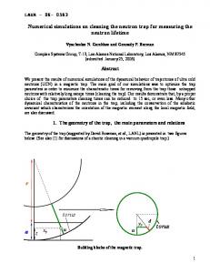
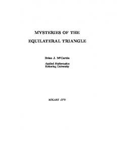
Figure 2.1: The geometric framework 1. The group W has six elements; it is isomorphic to the symmetric group in three letters S3 . 2. The group W acts simply transitively on the connected components of E2 \L1 ∪L2 ∪L3 (the Weyl chambers). 3. The group Wa is the semi-direct product Γ o W . A fundamental domain for the action of Wa on E2 is the closed equilateral triangle T , with vertices O = (0, 0), √ 3 1 A = (1, 0), and B = ( 2 , 2 ). 4. The group W acts simply transitively on the equilateral triangles which tile the regular hexagon [A, B, . . . , E, F ]. 5. The closed regular hexagon [A, B, . . . , E, F ] is a fundamental domain for the action of the lattice Γ on E2 . Proof. (1) Clearly, s21 = 1 (where 1 is the identity), s22 = 1, s23 = 1, and s3 = s1 ◦s2 ◦s1 = s2 ◦s1 ◦s2 . Furthermore, s1 ◦ s2 , s3 ◦ s1 and s2 ◦ s3 are equal to the rotation with center O and angle 2π ; s2 ◦ s1 , s1 ◦ s3 and s3 ◦ s2 are equal to the rotation with center O and angle − 2π . It 3 3 follows that W = {1, s1 , s2 , s3 , s1 ◦ s2 , s2 ◦ s1 } . To see that W is isomorphic to S3 , look at its action on the lines R αi , i = 1, 2, 3 . (2) Clear. (3) Write the action of (γ, σ) ∈ Γ × W on E2 , as x 7→ (γ, σ) · x = σ(x) + γ . 4

Then, (γ, σ).(γ 0 , σ 0 ) = (γ + σ(γ 0 ), σ ◦ σ 0 ). Clearly, si,k can be written as (kαi∨ , si ) and hence, Wa ⊂ Γ o W . To prove the reverse inclusion, we first remark that si (αi∨ ) = −αi∨ , and that s1 (α2∨
) = s2 (α1∨ ) = α1∨ + α2∨ . Note also that for m, n ∈ Z, we have si,m ◦ si,n = (m − n)αi∨ , 1 . One can then write (mα1∨ + nα2∨ , s1 ) = s2,n ◦ s2 ◦ s1,m , and (mα1∨ + nα2∨ , s2 ◦ s1 ) = s2 ◦ s2,m ◦ s2,n ◦ s1,m , and similar identities to conclude. √The fact that the equilateral triangle with vertices O = (0, 0), A = (1, 0), and B = ( 21 , 23 ) is a fundamental domain for Wa follows from the fact that the sides of the triangle are supported by the lines L1 , L2 and L3,1 . (4) Clear. (5) This assertion is illustrated by Figure 2.2. More precisely, we have the following correspondences of triangles which move the hexagon onto the fundamental domain {xα1∨ + yα1∨ | 0 ≤ x, y ≤ 1} for the action of Γ on E2 . Triangle [0, b, C] [0, C, c] [0, c, D] [0, D, d] [0, d, E] [0, E, e] [0, e, F ] [0, F, f ]

sent to [g, h, A] [g, A, f ] [i, j, B] [i, B, a] [i, a, A] [i, A, h] [k, b, B] [k, B, j]

by α1∨ α1∨ α3∨ α3∨ α3∨ α3∨ α2∨ α2∨ 

3 3.1

The equilateral torus Preliminaries

The equilateral torus is the flat torus T = E2 /Γ, where Γ is the lattice Z α1∨ Let Γ∗ be the dual lattice (see the notation P (R) in [5, 1])  Γ∗ = x ∈ E2 | hx, γi ∈ Z, ∀γ ∈ Γ .

L

Z α2∨ .

(3.1)

The lattice Γ∗ admits the basis {$1 , $2 }, where 1 1 2 $1 = ( , 0), $2 = ( , √ ), 3 3 3 which is dual to the basis {α1∨ , α2∨ } of Γ. 5

(3.2)

Figure 2.2: The hexagon is a fundamental domain for Γ Up to normalization, a complete set of eigenfunctions of the torus T is given by φp (x) = exp(2iπhx, pi),

(3.3)

where p ranges over Γ∗ , and x ∈ E2 . More precisely, for p ∈ Γ∗ , the function φp satisfies −∆φp = 4π 2 |p|2 φp . Writing p = m$1 + n$2 , we find that the eigenvalues of the equilateral torus T are the numbers 16π 2 2 ˆ (m + mn + n2 ), for m, n ∈ Z . (3.4) λ(m, n) = 9 ˆ The multiplicity of the eigenvalue λ(m, n) is the number  # (i, j) ∈ Z2 | i2 + ij + j 2 = m2 + mn + n2 . As usual the counting function NT (λ) of the torus T is defined by NT (λ) = # {n ≥ 1 | λn (T) < λ} , n o 2 2 2 = # (m, n) ∈ Z2 | 16π (m + mn + n ) < λ . 9 Lemma 3.1 The counting function of the equilateral torus satisfies √ 3 3 λ 9√ − λ + 1. NT (λ) ≥ 2 4π 2π

6

(3.5)

(3.6)

Figure 3.1: Illustration of (3.11) Proof. The lemma follows from easy counting arguments. Define the sets1 C = {x$1 + y$2 | x, y > 0} , C1 = {x$1 + y$2 | x, y > 1} ,

(3.7)

B(r) = {x ∈ E2 | |x| < r} . For (i, j) ∈ Z2 , define the closed lozenge Li,j , Li,j = {x$1 + y$2 | i ≤ x ≤ i + 1, j ≤ y ≤ j + 1} . Define the sets

(3.8)

L(r) = {(i, j) ∈ Z2 | i$1 + j$2 ∈ B(r)} , L2 (r) = {(i, j) ∈ Z2 | i$1 + j$2 ∈ C ∩ B(r)} ,

(3.9)

L1 (r) = {i ∈ Z | i ≥ 1 and i$1 ∈ B(r)} . Denote by A(Ω) the area of the set Ω contained in E2 or T. Define h$ to be the height of the equilateral triangle (0, $1 , $2 ), i.e., h$ = √13 , and define A$ to be the area of the lozenges Li,j . For symmetry reasons, we have the relation #L(r) = 6 #L2 (r) + 6 #L1 (r) + 1 . Furthermore, see Figure 3.1, it is easy to check, that [ C1 ∩ B(r) ⊂ Li,j . (i,j)∈L2 (r) 1

The set C is an open Weyl chamber [5].

7

(3.10)

(3.11)

It follows that A$ #L2 (r) ≥ A(C1 ∩ B(r)), and hence that A$ #L2 (r) ≥ A(C ∩ B(r)) − 2rh$ + A$ . Using the fact that h$ =

√1 3

and A$ =

2 √ , 3 3

we obtain that

√

3π 2 r − 3r + 1 . 4

(3.12)

 3 r ≥ r − 1. #L1 (r) = |$1 | 2

(3.13)

√ 3 3π 2 #L(r) ≥ r − 9r + 1 . 2

(3.14)

#L2 (r) ≥ Similarly, since |$1 | = 32 , we have that 

Finally, we obtain

√

Since NT (λ) = #L( 2πλ ), we obtain the estimate √ 3 3 λ 9√ NT (λ) ≥ λ + 1. − 2 4π 2π

(3.15) 

Remark. Notice that the area of the equilateral torus is √ 3 3 A(T) = , 2 so that the above lower bound is asymptotically sharp (Weyl’s asymptotic law). Denote by a(T) the length of the shortest closed geodesic on the flat torus T i.e., √ 3 ∨ 3 a(T) = |α1 | = . (3.16) 2 2 According to [10, §7], we get in the particular case of the torus the following isoperimetric inequality 2

Lemma 3.2 If a domain Ω ⊂ T has area A(Ω) ≤ (a(T)) , then the length `(∂Ω) of its π boundary satisfies `2 (∂Ω) ≥ 4πA(Ω) . Together with (3.16), this implies the Proposition 3.3 Let Ω ⊂ T be a domain whose area satisfies A(Ω) ≤ first Dirichlet eigenvalue of Ω satisfies the inequality λ(Ω) ≥

2 πj0,1 , A(Ω)

where j0,1 is the first positive zero of the Bessel function of order 0. 8

9 . 4π

Then, the

(3.17)

We recall that j0,1 ∼ 2.4048255577. Proof. Apply the proof of the classical Faber-Krahn inequality given for example in [7]. 

3.2

Courant-sharp eigenvalues of the equilateral torus

If λn = λn (T) is Courant-sharp, then λn−1 (T) < λn (T) and hence NT (λn ) = n − 1. In view of Lemma 3.1, we obtain √ 9p 3 3 λn − λn − (n − 2) ≤ 0 . 8π 2π It follows that s λn (T) Courant-sharp ⇒ λn (T) ≤ 12 1 +

2π 1 + √ (n − 2) 9 3

!2 .

(3.18)

If λn is Courant-sharp, there exists an eigenfunction u associated with λn with exactly n nodal domains. One of them, call it Ω, satisfies √ 3 3 A(T) = . A(Ω) ≤ n 2n If n ≥ 4, Ω satisfies the assumption of Proposition 3.3 and hence, 2 πj0,1 λn (T) = λ(Ω) ≥ . A(Ω)

It follows that n ≥ 4 and λn (T) Courant-sharp ⇒ λn (T) ≥

2 2πj0,1 √ n. 3 3

(3.19)

Comparing (3.18) and (3.19), we see that if the eigenvalue is Courant-sharp, then n ≤ 63 . Hence it remains to examine condition (3.19) for the first 63 eigenvalues. ¯ k such that The following table gives the first 85 normalized eigenvalues λ λk =

16π 2 ¯ λk . 9

The condition (3.19) becomes ¯ n (T) λ n ≥ 4 and λn (T) Courant-sharp ⇒ ≥ n

√ 2 3j0,1 ∼ 0.3985546913 . 8π

(3.20)

¯ the second column the The first column in the table displays the normalized eigenvalue λ; ¯ ¯ ¯ k = λ; ¯ least integer k such that λk = λ; the third column the largest integer k sur that λ ¯ The last column displays the ratio λ ¯ k /k which the fourth column the multiplicity of λ. should be larger than 0.3985546913 provided that n ≥ 4 and λn is Courant-sharp. 9

eigenvalue 0 1 3 4 7 9 12 13 16 19 21

minimum index maximum index multiplicity 1 1 1 2 7 6 8 13 6 14 19 6 20 31 12 32 37 6 38 43 6 44 55 12 56 61 6 62 73 12 74 85 12

ratio

0.3750000000 0.2857142857 0.3500000000 0.2812500000 0.3157894737 0.2954545455 0.2857142857 0.3064516129 0.2837837838

¯ n (T)/n is meaningful to study Courant-sharpness for n ≥ 4 only. Remark. The ratio λ This is why this information is not calculated in the first two lines.

4

The equilateral triangle: spectrum and action of symmetries

In this section, we start the analysis of the case of the equilateral triangle by recalling its spectrum and exploring the action of symmetries in each eigenspace of multiplicity 2. We keep the notation of the previous sections.

4.1

Eigenvalues and eigenfunctions

Recall the following result [1, Proposition 9]. Proposition 4.1 Up to normalization, a complete set of eigenfunctions of the Dirichlet Laplacian in the equilateral triangle T = {0, A, B}, with sides of length 1, is given by the functions P Φp = w∈W (w)φw(p) , (4.1) P Φp (x) = (w) exp (2iπhx, w(p)i) , w∈W where p ranges over the set C ∩Γ∗ , and where (w) is the determinant of w. The associated eigenvalues are the numbers 4π 2 |p|2 for p ∈ C ∩ Γ∗ . The multiplicity of the eigenvalue 4π 2 |p|2 is given by #{q ∈ C ∩ Γ∗ | |q| = |p|}. Remark. Notice that C ∩ Γ∗ = {m$1 + n$2 | m, n ∈ N• } , so that the eigenvalues of the equilateral triangle T , with sides of length 1, are the numbers 16π 2 2 (m + mn + n2 ) for m, n ∈ N• . 9 10

Figure 4.1: Parametrization F Idea of the proof. We follow [1]. Given a Dirichlet eigenfunction φ of the triangle, we extend it to a function ψ on E2 using the symmetries si,k , in such a way that ψ ◦ w = (w)ψ for any w in the group Wa . This is possible because T is a fundamental domain for Wa . The function ψ turns out to be smooth. Because Wa = Γ o W , the function ψ is Γ-periodic, and hence defines an eigenfunction Φ on the torus E2 /Γ which satisfies Φ ◦ w = (w)Φ for all w ∈ W . Conversely, any eigenfunction Φ on the torus, which satisfies this condition, gives a Dirichlet eigenfunction of the triangle. It remains to identify the eigenfunctions of the torus which satisfy the condition. This is done by making use of [5, Proposition 1, §VI.3].  The Dirichlet eigenfunctions of T look a little simpler in the following parametrization F of E2 , F : R2 → E2 , (4.2) F : (s, t) 7→ sα1∨ + tα2∨ . Given a point p ∈ E2 , we will denote by (x, y) its coordinates with respect to the standard basis {e1 , e2 }, and by (s, t)F its coordinates in the parametrization F. More precisely, we will write,  p = (x, y), for p = xe1 + ye2 , (4.3) p = (s, t)F for p = sα1∨ + tα2∨ . In the parametrization F, a fundamental domain for the action of Γ on R2 is the square {0 ≤ s ≤ 1} × {0 ≤ t ≤ 1}; a fundamental domain for the action of Wa on R2 is the triangle with vertices (0, 0)F , ( 32 , 13 )F and ( 31 , 23 )F , see Figure 4.1. Notice that the parametrization F is not orthogonal, and that the Laplacian is given in this parametrization by
4 2 2 ∆F = ∂ss + ∂st + ∂tt2 . (4.4) 9 Recall that the function φp is defined by φp (x) = exp (2iπhx, pi), for x ∈ E2 and p ∈ Γ. In the parametrization F, writing x = sα1∨ + tα2∨ and p = m$1 + n$2 , the function φp 11

will be written as φm,n (s, t) = exp (2iπ(ms + nt)) .

(4.5)

To write the eigenfunctions of the Dirichlet Laplacian in the equilateral triangle, we have to compute the scalar products hx, w(p)i or equivalently hw(x), pi for x = sα1∨ + tα2∨ and p = m$1 + n$2 . Table 4.1 displays the result. w

det(w)

hw(x), pi

1

1

ms + nt

s1

−1 −ms + (m + n)t

s2

−1

(m + n)s − nt

s3

−1

−ns − mt

s1 ◦ s2

1

ns − (m + n)t

s2 ◦ s1

1 −(m + n)s + mt

Table 4.1: Action of W Define the functions



Em,n (s, t) = exp 2iπ ms + nt − exp 2iπ − ms + (m + n)t



− exp 2iπ (m + n)s − nt − exp 2iπ − ns − mt



+ exp 2iπ ns − (m + n)t + exp 2iπ − (m + n)s + mt ,

(4.6)

Using Table 4.1, we see that En,m (s, t) = −Em,n (s, t) .

(4.7)

Looking at the pairs [m, n] and [n, m] simultaneously, and making use of real eigenfunctions instead of complex ones, we find that eigenfunctions associated with the pairs of positive integers [m, n] and [n, m], are Cm,n (s, t) and Sm,n (s, t), given by the following formulas,

Cm,n (s, t) = cos 2π ms + nt − cos 2π − ms + (m + n)t

− cos 2π (m + n)s − nt − cos 2π − ns − mt (4.8)

+ cos 2π ns − (m + n)t + cos 2π − (m + n)s + mt , and

Sm,n (s, t) = sin 2π ms + nt − sin 2π − ms + (m + n)t

− sin 2π (m + n)s − nt − sin 2π − ns − mt

+ sin 2π ns − (m + n)t + sin 2π − (m + n)s + mt .

(4.9)

Remarks. Notice that by (4.7) Cm,n = −Cn,m and Sm,n = Sn,m . The line {s = t} corresponds to the median of the equilateral triangle T issued from O. This median divides 12

T into two congruent triangles with angles {30, 60, 90} degrees. The eigenfunctions Cm,n correspond to the Dirichlet eigenfunctions of these triangles. When m = n, we have Cm,m ≡ 0 and Sm,m (s, t) = 2 {sin 2πm(s + t) − sin 2πm(2t − s) − sin 2πm(2s − t)} , i.e., Sm,m (s, t) = S1,1 (ms, mt) .

4.2

(4.10)

Symmetries

Call FC the centroid of the equilateral triangle T = {0, A, B}. With the conventions √ 3 1 (4.3), FC = ( 2 , 6 ) = ( 13 , 31 )F . The isometry group GT of the triangle T has six elements: the three orthogonal symmetries with respect to the medians of the triangle (which fix one vertex and exchange the two other vertices), the rotations ρ± , with center FC and angles ± 2π (which permute the vertices), and the identity. The group GT fixes the centroid FC . 3 In the parametrization F, the symmetries are given by σ1 (s, t) = (t, s) , σ2 (s, t) = (−s + 32 , t − s + 13 ) , σ3 (s, t) = (s − t +

1 , −t 3

+

(4.11)

2 ). 3

i.e., respectively, the symmetries with respect to the median issued from 0, to the median issued from B, and to the median issued from A. As a matter of fact, the group GT is generated by the symmetries σ1 and σ2 . The rotations are 1 2 ρ+ = σ2 ◦ σ1 : (s, t) 7→ (−t + , s − t + ), 3 3 2π with angle 3 , and 1 2 ρ− = σ1 ◦ σ2 : (s, t) 7→ (t − s + , −s + ), 3 3 with angle − 2π . Furthermore, σ3 = σ1 ◦ σ2 ◦ σ1 = σ2 ◦ σ1 ◦ σ2 . 3 The action of the symmetries σ1 , σ2 on the eigenfunctions Cm,n and Sm,n is given by σ1∗ Cm,n = −Cm,n , σ1∗ Sm,n = Sm,n , σ2∗ Cm,n = − cos αm,n Cm,n − sin αm,n Sm,n , σ2∗ Cm,n = − sin αm,n Cm,n + cos αm,n Sm,n , where αm,n =

2π(2m+n) . 3

13

(4.12)

Working in the parametrization F and using the convention (4.3), we define for the 2 analysis of the zero set of any eigenfunction associated with 16π (m2 + mn + n2 ) (in the 9 case of multiplicity 2) the family Ψθm,n (s, t) = cos θ Cm,n (s, t) + sin θ Sm,n (s, t) .

(4.13)

The action of the symmetries on the family Ψθm,n defined by (4.13) is given by σ1∗ Ψθm,n = Ψπ−θ m,n , −θ

,

π−α −θ Ψm,n m,n

.

π+α

σ2∗ Ψθm,n = Ψm,n m,n σ3∗ Ψθm,n

5

=

(4.14)

Pleijel’s approach for Courant-sharp eigenvalues

In order to investigate the Courant-sharp Dirichlet eigenvalues of the equilateral triangle T , we use the same methods as in [16] and Section 3. Notice that the counting function of the Dirichlet eigenvalues of the equilateral triangle is given by √   λ λ • • 2 NT (λ) = L2 ( ) = # (k, `) ∈ N × N | |k$1 + `$2 | < 2 . (5.1) 2π 4π Using (3.12), we conclude that √ NT (λ) ≥

3 λ 3√ − λ + 1. 4 4π 2π

(5.2)

Notice that this lower bound is asymptotically sharp (Weyl’s asymptotic law). Assuming that λn (T ) is Courant-sharp, we have λn−1 (T ) < λn (T ), and hence NT (λn (T )) = n − 1. It follows that  2 r π λn (T ) Courant-sharp ⇒ λn (T ) ≤ 48 1 + 1 + √ (n − 2) . 3 3

(5.3)

On the other-hand, if λn (T ) is Courant-sharp, there exists an eigenfunction u with exactly n nodal domains Ω1 , . . . Ωn , for which we can write λn (T ) = λ(Ωi ) ≥

2 πj0,1 , A(Ωi )

where we have used the Faber-Krahn inequality in E2 . Summing up in i, it follows that λn (T ) Courant-sharp ⇒

2 2 πj0,1 4πj0,1 λn (T ) ≥ = √ . n A(T ) 3

14

(5.4)

Combining (5.3) and (5.4), we find that if λn (T ) is Courant-sharp, then n ≤ 40 . It follows that to determine the Courant-sharp eigenvalues, it suffices to look at the first ¯ 40 eigenvalues of the equilateral triangle. Using (5.4) again, we compute the ratios λnn(T ) ¯ n (T ) = 9 2 λn (T )), and compare them with the for the first 40 normalized eigenvalues (λ 16π value √ 2 3 3j0,1 ∼ 2.391328148 . 4π This is given by the following table in which the first column gives the normalized eigen¯ the second column the smallest index i such that λ ¯ i = λ; ¯ the third column the value λ; ¯ j = λ; ¯ the fourth column the multiplicity of λ; ¯ and the last largest index j such that λ one the ratio normalized eigenvalue/least index (which is the relevant information for checking the Courant-sharp property).

¯ λ 3 7 12 13 19 21 27 28 31 37 39 43 48 49 52 57 61 63 67 73 75 76 79

¯ i (T ) λ i

¯i = λ ¯ λ ¯j = λ ¯ mult(λ) ¯ λ 1 2 4 5 7 9 11 12 14 16 18 20 22 23 25 27 29 31 33 35 37 38 40

1 3 4 6 8 10 11 13 15 17 19 21 22 24 26 28 30 32 34 36 37 39 41

1 2 1 2 2 2 1 2 2 2 2 2 1 2 2 2 2 2 2 2 1 2 2

3 3.5 3 2.6000000 2.7142857 2.333333333 2.45454545 2.333333333 2.214285714 2.312500000 2.166666667 2.150000000 2.181818182 2.130434783 2.080000000 2.111111111 2.103448276 2.032258065 2.030303030 2.085714286 2.027027027 2. 1.975000000

Table 5.1: Courant-sharp eigenvalues satisfy

¯ n (T ) λ n

≥ 2.391328148

Lemma 5.1 The only possible Courant-sharp eigenvalues of the equilateral triangle are the λk (T ), for k ∈ {1, 2, 4, 5, 7, 11}.

15

ˆ 2) and Clearly, the eigenvalues λ1 and λ2 are Courant-sharp. The eigenvalues λ4 = λ(2, ˆ λ11 = λ(3, 3) are simple. It is easy to see that the number of nodal domains is 4, resp. 9, for these eigenvalues, see (4.10) and Figure 5.1. Hence λ4 is Courant sharp, and λ11 is not Courant sharp.

Figure 5.1: Nodal sets corresponding to λ4 and λ11 In order to determine the Courant-sharp eigenvalues, it therefore remains to consider the ˆ 3) = λ(3, ˆ 1) and λ7 = λ(2, ˆ 3) = λ(3, ˆ 2) which have multiplicity 2. eigenvalues λ5 = λ(1, We study these eigenvalues in Sections 7 and 8 respectively, see Figures 5.2 and 5.3.

Figure 5.2: Nodal sets for the eigenfunctions C1,3 and S1,3 corresponding to λ5 We will work in the triangle T , with vertices {O, A, B}. We denote by FC the centroid of the triangle. The median issued from the vertex O is denoted by [OM ], the mid-point of the side BA by MO . We use similar notation for the other vertices, see Figure 5.4. Remark. We denote by N (Ψθm,n ) the nodal set of the eigenfunction Ψθm,n i.e., the closure of the set of zeros of the eigenfunction in the interior of the triangle. The eigenfunctions also vanish on the edges of the triangles, and we will analyze separately the points in the open edges and the vertices. For a summary of the general properties of nodal sets of eigenfunctions, we refer to [4, Section 5]. Observe that the eigenfunctions Ψθm,n are defined over the whole plane, so that even at the boundary of the triangle, we can use the local structure of the nodal set.

16

Figure 5.3: Nodal sets for the eigenfunctions C2,3 and S2,3 corresponding to λ7 Point

E2

F

Vertex O

(0, 0)

(0, 0)F

Vertex A

(1, 0)

( 23 , 13 )F

Vertex B

( 12 ,

Centroid FC

( 12 ,

Mid-point MO

( 32 ,

Mid-point MA

( 12 ,

Mid-point MB

√

3 ) 2 √ 3 ) 6 √ 3 ) 4 √ 3 ) 4

( 12 , 0)

( 13 , 23 )F ( 13 , 13 )F ( 12 , 12 )F ( 16 , 13 )F ( 13 , 16 )F

Figure 5.4: Triangle T The remaining part of this paper is devoted to the proof of Theorem 1.2, using the following strategy.

6

Playing on the checkerboard

After the reduction a` la Pleijel, we now have to analyze the nodal picture of any eigenfunction in two 2-dimensional eigenspaces of the Laplacian in T , the interior of the equilateral triangle. The nodal set N (Ψ) of a Dirichlet eigenfunction Ψ is the closure of the set {x ∈ T | Ψ(x) = 0} in T . The function Ψ actually extends smoothly to the whole plane, and the nodal set of Ψ consists of finitely many regular arcs which may intersect, or hit the boundary of T , with the equiangular property, [9, Section 2.1]. Let λ be either λ5 or λ7 , and let E be the associated (2-dimensional) eigenspace. Determining whether λ is Courant-sharp amounts to describing the possible nodal sets of the family Ψθ = cos θ C + sin θ S, where {C, S} is a basis of E, and θ ∈ [0, 2π]. For this purpose, we use the following ideas. 1. Using the natural symmetries of the triangle, we restrict the analysis to θ ∈ [0, π6 ]. 17

π

Figure 6.1: Checkerboards for λ5 and λ7 , and nodal set N (Ψ 6 ) 2. The set of fixed points N (C) ∩ N (S) i.e., the set of common zeros of the functions Ψθ , plays an important role in the analysis of the family of nodal sets N (Ψ). When the variables are separated, as in the case of the square membrane, it is easy to determine the fixed points, [17, 4]. In the case of the equilateral triangle, we shall only determine the fixed points located on the medians of T . 3. For θ ∈]0, π6 ], the nodal set N (Ψθ ) is contained in the set {C S < 0}∪(N (C) ∩ N (S)), [17, 4]. This checkerboard argument is illustrated in Figure 6.1 which displays the π checkerboards for λ5 and λ7 , with C = Ψ0 and S = Ψ 2 , as well as the nodal set π of Ψ 6 (Maple simulations). For the equilateral triangle, the variables are not separated, and we shall not use this argument directly, but rather separation lemmas involving the medians and other natural lines. 4. Critical zeros i.e., points at which both the eigenfunction and its first derivatives vanish, play a central role in our analysis. They are easy to determine when the variables are separated, [4]. In the case of the equilateral triangle, the determination of critical zeros is more involved. We first analytically determine the critical zeros on the boundary i.e., the points at which the nodal sets hits ∂T . Later on in the proof, we show that Ψθ does not have interior critical zeros when θ ∈]0, π6 ]. For this purpose, we use the following energy argument. 5. Energy argument. The medians divide the triangle T into six isometric semiequilateral triangles, whose first Dirichlet eigenvalue is easily seen to be strictly larger than λ7 . This argument is needed to discard possible interior critical zeros, and also simply closed nodal arcs. For a given θ ∈]0, π6 ], the above information provide some points in N (Ψθ ). It remains to determine how the nodal arcs can join these points, without crossing the established barriers.

18

7

The eigenvalue λ5(T ) and its eigenspace

We call E5 the 2-dimensional eigenspace associated with the eigenvalue λ5 (T ), i.e., with the pairs [1, 3] and [3, 1]. Recall the eigenfunctions, C1,3 (s, t) = cos 2π(s + 3t) − cos 2π(−s + 4t) − cos 2π(4s − 3t) − cos 2π(−3s − t) + cos 2π(3s − 4t) + cos 2π(−4s + t) , S1,3 (s, t) = sin 2π(s + 3t) − sin 2π(−s + 4t) − sin 2π(4s − 3t) − sin 2π(−3s − t) + sin 2π(3s − 4t) + sin 2π(−4s + t) .

(7.1)

In this section, we now study the family Ψθ1,3 more carefully.

7.1

Symmetries

Taking Subsection 4.2 into account, we find that σ1∗ Ψθ1,3

= Ψπ−θ 1,3 ,

σ2∗ Ψθ1,3

3 = Ψ1,3 ,

σ3∗ Ψθ1,3

3 = Ψ1,3

π

−θ

5π

−θ

2π +θ 3

(σ2 ◦ σ1 )∗ Ψθ1,3 = Ψ1,3

4π +θ 3

(σ1 ◦ σ2 )∗ Ψθ1,3 = Ψ1,3

,

(7.2)

, .

It follows that, up to multiplication by a scalar, and for V ∈ {O, A, B} , the eigenspace E5 contains a unique eigenfunction SV , resp. a unique eigenfunction CV , which is invariant, resp. anti-invariant, under the symmetry σi(V ) with respect to the median [V M ] issued from the vertex V , where i(O) = 1, i(A) = 3 , and i(B) = 2 . More precisely, we have π

2 and CO = Ψ01,3 , SO = Ψ1,3 11π

4π

3 SA = Ψ1,36 and CA = Ψ1,3 , 7π

(7.3)

2π

6 3 SB = Ψ1,3 and CB = Ψ1,3 .

Note that CO , resp. SO , are the functions C1,3 , resp. S1,3 , and that, SA = (σ1 ◦ σ2 )∗ SO and CA = (σ1 ◦ σ2 )∗ CO , SB = (σ2 ◦ σ1 )∗ SO and CB = (σ2 ◦ σ1 )∗ CO .

(7.4)

The eigenfunctions SV , resp. CV , are permuted under the action of the rotations ρ+ = σ2 ◦ σ1 and ρ− = σ1 ◦ σ2 . The eigenspace E5 does not contain any non trivial rotation invariant eigenfunction. θ Since Ψθ+π 1,3 = −Ψ1,3 , it follows from (7.2) that, up to the symmetries σi , the nodal sets of the family Ψθ1,3 , θ ∈ [0, 2π] are determined by the nodal sets of the sub-family θ ∈ [0, π6 ] .

From now on, we assume that θ ∈ [0, π6 ]. 19

7.2

Behaviour at the vertices

The vertices of the equilateral triangle T belong to the nodal set N (Ψθ1,3 ) for all θ. For geometric reasons, the order of vanishing at a vertex is at least 3. More precisely, Properties 7.1 Behaviour of Ψθ1,3 at the vertices. 1. The function Ψθ1,3 vanishes at order 6 at O if and only if θ ≡ 0 (mod π); otherwise it vanishes at order 3. 2. The function Ψθ1,3 vanishes at order 6 at A if and only if θ ≡ it vanishes at order 3.

π 3

(mod π); otherwise

3. The function Ψθ1,3 vanishes at order 6 at B if and only if θ ≡ it vanishes at order 3.

2π 3

(mod π); otherwise

In other words, up to multiplication by a scalar, the only eigenfunction Ψθ1,3 which vanishes at higher order at a vertex V ∈ {O, A, B} is CV , the anti-invariant eigenfunction with respect to the median issued from the vertex V . In particular, when θ ∈]0, π6 ], the three vertices are critical zeros of order three for the eigenfunction Ψθ1,3 , and no interior nodal curve of such an eigenfunction can arrive at a vertex. Proof. Compute the Taylor expansions of Ψθ1,3 at the points under consideration.

7.3



Fixed points on the medians

Since the median [OM ] is contained in the nodal set N (C1,3 ), the intersection points of [OM ] with N (S1,3 ) are fixed points of the family N (Φθ1,3 ), i.e., common zeros of the functions Ψθ1,3 . If we parametrize [OM ] by u 7→ (u, u) with u ∈ [0, 12 ], we find that S1,3 [OM ] (u) = 2 sin(8πu) − 2 sin(6πu) − 2 sin(2πu) . (7.5) It follows that S1,3 [OM ] (u) = −8 sin(πu) sin(3πu) sin(4πu) .

(7.6)

The last formula shows that there are two fixed points on the open median [OM ], the centroid of the triangle FC = ( 31 , 13 )F , and the point FO = ( 14 , 14 )F . Taking into account the action of GT on the space E5 , see (7.2)-(7.4), we infer that the 5 1 5 points FA = ( 12 , 3 )F and FB = ( 13 , 12 )F are also common zeros for the family Ψθ1,3 . They are deduced from FO by applying the rotations ρ± , and situated on the two other medians. Using Taylor expansions, it is easy to check that the fixed points F∗ are not critical zeros of the functions Ψθ1,3 . In the neighborhood of the fixed points F∗ , the nodal set consists of a single regular arc. Remarks. (i) Note that we do not claim to have determined all the fixed points of the family 20

Point

E2

F

Vertex O

(0, 0)

(0, 0)F

Vertex A

(1, 0)

( 23 , 13 )F

Vertex B

( 21 ,

Fixed point FC

( 21 ,

Fixed point FO

( 83 ,

Fixed point FA

( 85 ,

Fixed point FB

( 21 ,

√ 3 ) 2 √ 3 ) 6 √ 3 ) 8 √ 3 ) 8 √ 3 ) 4

( 13 , 23 )F ( 13 , 13 )F ( 14 , 14 )F 5 1 ( 12 , 3 )F 5 ( 13 , 12 )F

Figure 7.1: Triangle T and fixed points for Ψθ1,3 N (Ψθ1,3 ) i.e., the set N (C1,3 ) ∩ N (S1,3 ). We have so far only determined the fixed points located on the medians. (ii) Notice that the fixed point FO is the mid-point of the segment [MA MB ], etc .

7.4

Partial barriers for the nodal sets

We have seen that the family Ψθ1,3 has four fixed points, the centroid FC of the triangle, and three other points FO , FA and FB , located respectively on the open medians [OM ], [AM ], and [BM ], see Figure 7.1. As a matter of fact, the medians can serve as partial barriers. Lemma 7.2 For any θ, the nodal set N (Ψθ1,3 ) intersects each median at exactly two points unless the function Ψθ1,3 is one of the functions CV for V ∈ {O, A, B}, in which case the corresponding median is contained in the nodal set. In particular, if θ ∈]0, π6 ], the nodal set N (Ψθ1,3 ) only meets the medians at the fixed points {FO , FA , FB , FC }. Proof. Use the following facts: (i) the families {CO , SO }, {CA , SA } and {CB , SB } span E5 ; (ii) the function CV vanishes on the median issued from the vertex V . Write Ψθ1,3 = αCV + βSV . If x ∈ [V M ] ∩ N (Ψθ1,3 ), then βSV (x) = 0. If β 6= 0, then x ∈ {FC , FV }. If β = 0, then [V M ] ⊂ N (Ψθ1,3 ).  Remark. A consequence of Lemma 7.2 and Subsection 7.3 is that for θ ∈]0, π6 ], no critical zero of the function Ψθ1,3 can occur on the medians. The medians divide the equilateral triangle T into six isometric H-triangles (i.e., triangles with angles {30, 60, 90} degrees), T (FC , O, MB ), etc . Each one of theses triangles is homothetic to the H-triangle T (O, A, MO ) with scaling factor √13 . On the other-hand, the first Dirichlet eigenvalue for the H-triangle T (O, A, MO ) is λ2 (T ) = 7, with multiplicity 1, and associated eigenfunction C1,3 . 21

Lemma 7.3 Let TM denote the triangle T (FC , O, MB ). The first Dirichlet eigenvalue of the six H-triangles determined by the medians of T equals λ(TM ) = 3λ2 (T ) = 21 . For 0 ≤ a ≤ 1, define the line Da by the equation s + t = a in the parametrization F. Da = F ({s + t = a}) .

(7.7)

Lemma 7.4 For a ∈ { 21 , 23 , 34 }, the intersections of the lines Da with the nodal sets N (C1,3 ) and N (S1,3 ) are as follows. D 1 ∩ N (C1,3 ) = {FO }, 2 D 2 ∩ N (C1,3 ) = {FC , GA , GB }, 3 D 3 ∩ N (C1,3 ) = {FA , FB , GO }, 4

and and and

D 1 ∩ N (S1,3 ) = {FO }, 2 D 2 ∩ N (S1,3 ) = {FC }, 3 D 3 ∩ N (S1,3 ) = {FA , FB },

(7.8)

4

where GA and GB are symmetrical with respect to [OM ], and GO = ( 83 , 38 )F . The lines are tangent to N (S2,3 ) at the points FO and FC . Proof. The segment Da ∩ T is parametrized by u 7→ (u, a − u) for u ∈ [ a3 , 2a ]. For each 3 value a ∈ { 12 , 23 , 34 }, define BCa (u) = C2,3 (u, a − u), u ∈ [ a3 , 2a ], 3 a 2a BSa (u) = S2,3 (u, a − u), u ∈ [ 3 , 3 ] .

(7.9)

BC 1 (u) = −4 sin(2πu) sin(12πu) , 2 BS 1 (u) = 4 cos(2πu) sin(12πu) .

(7.10)

√ BC 2 (u) = −2 3 sin(9πu) cos(5πu + π3 ) , 3 √ BS 2 (u) = −2 3 sin(9πu) sin(5πu + π3 ) .

(7.11)

BC 3 (u) = −2 sin(12πu) (sin(2πu) + cos(2πu)) , 4 BS 3 (u) = −2 sin(12πu) (sin(2πu) − cos(2πu)) .

(7.12)

Taking a = 21 , we find

2

Similarly,

5

4

Looking at the zeros of the above functions in the respective intervals, the lemma follows.  The lemmas are illustrated by Figure 7.2 which displays the partial barriers (thin segments), and the nodal sets computed with Maple (thicker lines).

22

Figure 7.2: Partial barriers for N (C1,3 ) and N (S1,3 )

7.5

Critical zeros of C1,3 and S1,3 on the sides of T , and on the median [OM ]

Define the functions F C(u) := − sin(7πu) + 3 sin(5πu) − 4 sin(2πu) , F S(u) := − cos(7πu) − 3 cos(5πu) + 4 cos(2πu) ,

(7.13)

and the polynomials PC (x) := 4x2 + 4x − 1 , PS (x) := 4x4 − x2 + x − 1 .

(7.14)

Lemma 7.5 The functions F C and F S satisfy, F C(u) = −4 sin(πu) (cos(πu) − 1)2 (2 cos(πu) + 1)2 PC (cos(πu)) , F S(u) = −4 (cos(πu) − 1) (2 cos(πu) + 1)2 PS (cos(πu)) . Proof. Use the Chebyshev polynomials.

(7.15) 

Properties 7.6 The partial derivatives of the functions C1,3 and S1,3 satisfy the following relations. 1. Parametrize the edge [OA] by u 7→ (u, u/2), with u ∈ [0, 2/3]. Then, ∂s C1,3 (u, u/2) = 2πF C(u) , ∂t C1,3 (u, u/2) = −4πF C(u) , ∂s S1,3 (u, u/2) = 2πF S(u) , ∂t S1,3 (u, u/2) = −4πF S(u) .

(7.16)

2. Parametrize the edge [OB] by u 7→ (u/2, u), with u ∈ [0, 2/3]. Then, ∂s C1,3 (u/2, u) = 4πF C(u) , ∂t C1,3 (u/2, u) = −2πF C(u) , ∂s S1,3 (u/2, u) = −4πF S(u) , ∂t S1,3 (u/2, u) = 2πF S(u) . 23

(7.17)

3. Parametrize the edge [BA] by u 7→ (u/2, 1 − u/2), with u ∈ [2/3, 4/3]. Then, ∂s C1,3 (u/2, 1 − u/2) = −2πF C(u) , ∂t C1,3 (u/2, 1 − u/2) = −2πF C(u) , ∂s S1,3 (u/2, 1 − u/2) = 2πF S(u) , ∂t S1,3 (u/2, 1 − u/2) = 2πF S(u) .

(7.18)

Proof. It suffices to compute the partial derivatives of C1,3 and S1,3 , and to make the substitutions corresponding to the parametrization of the edges.  It follows from the above results that the critical zeros of C1,3 , resp. S1,3 , on ∂T are determined by the zeros of F C, resp. F S, in [0, 4/3]. Lemma 7.7 Zeros of PC and PS . √ 1. The polynomial PC has only one root in the interval [−1, 1] , namely ( 2 − 1)/2 . 2. The polynomial PS has exactly two roots in the interval [−1, 1], namely ξ− ≈ −0.9094691258 and ξ+ ≈ 0.6638481772 . Define the numbers u1,C := u1,S := u2,S :=

√ 2−1 1 arccos( ) ≈ 0.433595245 , π 2 1 arccos(x+ ) ≈ 0.2689221041 , π 1 arccos(x− ) ≈ 0.8635116189 , π

(7.19)

u3,S := 2 − u2,S ≈ 1.136488381 . The function F C vanishes at 0, 23 , 1 and 43 , and has one simple zero u1,C ∈]0, 32 [. The function F S vanishes at 0, 32 and 34 . It has one simple zero u1,S ∈]0, 32 [, and two simple zeros u2,S , u3,S ∈] 23 , 43 [ . Properties 7.8 Critical zeros of the functions C1,3 and S1,3 on the open edges of T . 1. The function C1,3 has one critical zero Z1,C = (u1,C , u1,C /2)F on the open edge [OA]; one critical zero Z2,C = (u1,C /2, u1,C )F on the open edge [OB]; one critical zero Z3,C = MO = (1/2, 1/2)F on the open edge [BA]. These critical zeros have order 2. 2. The function S1,3 has one critical zero Z1,S = (u1,S , u1,S /2)F on the open edge [OA]; one critical zero Z2,S = (u1,S /2, u1,S )F on the open edge [OB]; two critical zeros Z3,S = (u2,S /2, 1 − u2,S /2)F and Z4,S = (u3,S /2, 1 − u3,S /2)F on the open edge [BA], these points are symmetrical with respect to the point MO . These critical zeros have order 2 . Proof. Use Properties 7.6 and Lemma 7.7.



Remark. The vertex O is a critical zero of order 6 of C1,3 , and a critical zero of order 3 of S1,3 . The vertices A and B are critical zeros of order 3 of both C1,3 and S1,3 , see Properties 7.1. 24

Properties 7.9 Critical zeros of the functions C1,3 and S1,3 on the median [OMO ]. 1. The function C1,3 has one critical zero at O; one critical zero Z5,C of order 2 , where Z5,C = (u5,C /2, u5,C /2)F , with u5,C := 1 − arccos(3/4)/π ≈ 0.7699465439 ; one critical zero MO = Z3,C of order 2 . 2. The function S1,3 has no critical zero on the median [OM ], except the point O. Proof. Since C1,3 vanishes on the median, its critical zeros on the median are the common zeros of its partial derivatives. They are precisely the zeros of the function 2 sin(4πu) − 5 sin(3πu) + 7 sin(πu) , if we parametrize the median by u 7→ (u/2, u/2) for u ∈ [0, 1]. The above function can be factorized as

2 4 sin(πu) 4 cos(πu) + 3 cos(πu) − 1 , and the first assertion follows. For the second assertion, we have to look for the common zeros of the function S1,3 and its derivatives on the median. This amounts to finding the common zeros of the functions 2 sin(4πu) − 2 sin(3πu) − 2 sin(πu) , and 4 cos(4πu) − 3 cos(3πu) − cos(πu) . The first function factorizes as −8 sin(

3πu πu ) sin( ) sin(2πu) . 2 2

It is easy to check that the only common zero is u = 0 . Figure 7.3 displays the critical zeros of C1,3 and S1,3 . We state the following corollary of Proposition 7.9 for later reference. π

6 Recall (see the notation (7.3)) that Ψ1,3 = −SB , and that SB = ρ∗+ SO .

Corollary 7.10 Critical zeros of the function SB . 1. The function SB has two critical zeros of order 2 on the side [OA], Z3,SB = ρ− (Z3,S ) and Z4,SB = ρ− (Z4,S ) . 2. The function SB has one critical zero of order 2 on the side [OB], Z1,SB = ρ− (Z1,S ) . 3. The function SB has one critical zero of order 2 on the side [BA], Z2,SB = ρ− (Z2,S ) . 25



Point

E2

Z1,C

≈ (0.6504, 0)

Z2,C

≈ (0.3252, 0.5633) ( 34 ,

Z3,C

F (u1,C , (

√

u1,C 2

3 ) 4

Z5,C

≈ (0.5775, 0.3334)

Z1,S

≈ (0.4034, 0)

Z2,S

≈ (0.2017, 0.3494)

Z3,S

≈ (0.6476, 0.6104)

Z4,S

≈ (0.8524, 0.2507)

u1,C )F 2

, u1,C )F

( 12 , 12 )F (

u5,C 2

,

(u1,S ,

u5,C )F 2 u1,S ) 2 F

u1,S , u1,S )F 2 u u ( 2,S , 1 − 2,S ) 2 2 F u u , 1 − 3,S ) ( 3,S 2 2 F

(

Figure 7.3: Fixed points and critical zeros for C1,3 and S1,3

7.6

The nodal sets of C1,3 and S1,3

Properties 7.11 Nodal sets of C1,3 and S1,3 . 1. The function C1,3 has only one critical zero Z5,C in the interior of the triangle. Its nodal set consists of the diagonal [OMO ], and a regular arc from Z1,C to Z2,C which intersects [OMO ] orthogonally at Z5,C , and passes through FA and FB . 2. The function S1,3 has no critical zero in the interior of the triangle. Its nodal set consists of two disjoint regular arcs, one from Z1,S to Z2,S , passing through FO ; one from Z3,S to Z4,S , passing through FB and FA . Proof. We have determined the common zeros of C1,3 and S1,3 located on the medians (Subsection 7.3), as well as the critical zeros on the open edges of the triangle T and on the medians [OM ] (Subsection 7.5). We already know the local behaviour at the vertices (Subsection 7.2). Using Subsection 7.4, we also know that the nodal set N (C1,3 ) only meets the medians at the fixed points and at Z5,C , and that the nodal set N (S1,3 ) only meets the medians at the fixed points. Looking at the Taylor expansions, we can determine the local nodal patterns of C1,3 and S1,3 near the fixed points and near the critical zeros, see Figure 7.4. This figure also displays the medians, and takes into account the fact that [OM0 ] ⊂ N (C1,3 ). The medians divide T into six isometric H-triangles, Figure 7.3. The nodal sets of C1,3 and S1,3 consist of finitely many nodal arcs which are smooth except at the critical zeros. They can only exit the interior of an H-triangle at a fixed point or at a critical zero, according to the local nodal patterns shown in Figure 7.4. Claim. The functions C1,3 and S1,3 cannot have any critical zero in the interiors of the H-triangles. Indeed, assume there is one critical zero Z in the interior of some H-triangle H. At this point, the nodal set would consist of at least four semi-arcs. Following any such semi-arc, 26

we either obtain a simply closed nodal arc, or exit the triangle. Since there are at most three exit points (with only one exit direction at each point), there would be at least one simply closed nodal component in the interior of the triangle H. This component would bound at least one nodal domain ω. The first Dirichlet eigenvalue λ(ω) would satisfy λ(ω) = λ5 (T ) = 13. On the other-hand, since ω is contained in the interior of H, we would have λ(ω) > λ(H) = 21 according to Lemma 7.4. This proves the claim by contradiction. The last argument in the proof of the claim also shows that the interiors of the H-triangles cannot contain any closed nodal component. This shows that the nodal sets of C1,3 and S1,3 are indeed as shown in Figure 5.2.  Remark. Here is another argument to determine the nodal set N (C1,3 ). The claim is that C1,3 cannot have a second interior critical zero. Indeed, such a critical zero would be of order at least 2, and cannot belong to the median [OM ], so that it must belong to one of the two H-triangles determined by this median. For symmetry reasons, we would have at least one critical zero in each of these H-triangles. The eigenvalue λ5 (T ) which corresponds to the pairs [1, 3] and [3, 1] is also the second Dirichlet eigenvalue of these triangles, so that it has two nodal domains, Ω1 and Ω2 . Applying the Euler formula [3, (2.11)] to the nodal partition D = (Ω1 , Ω2 ), we would have 1 1 1 1 + (1 + 1 + 2) ≤ χ( T ) + σ(Ω1 , Ω2 ) = χ(Ω1 ) + χ(Ω2 ) ≤ 2 , 2 2 2 a contradiction.

Figure 7.4: Local nodal patterns for C1,3 (left) and S1,3 (right)

27

7.7

Critical zeros of Ψθ1,3 on the sides of T

As a consequence of Properties 7.6, the critical zeros of the functions Ψθ1,3 , for θ ∈]0, π6 ], on the sides of the triangle T are determined by one of the equations cos θ F C(u) ± sin θ F S(u) = 0 . Since θ ∈]0, π6 ], the vertices of T are critical zeros of order 3 of Ψθ1,3 (Properties 7.1). Since we are interested in the critical zeros on the open edges, we can substitute F C, resp. F S, by the functions GC, resp. GS, defined as follows. GC(u) := sin(πu) (cos(πu) − 1) (4 cos2 (πu) + 4 cos(πu) − 1) , GS(u) := 4 cos4 (πu) − cos2 (πu) + cos(πu) − 1 .

(7.20)

Properties 7.12 The critical zeros of the function Ψθ1,3 on the open edges of the triangle T are determined by the following equations. 1. On the edge [OA] parametrized by u 7→ (u, u/2), cos θ GC(u) + sin θ GS(u) = 0 , for u ∈ [0, 2/3] .

(7.21)

2. On the edge [OB] parametrized by u 7→ (u/2, u), cos θ GC(u) − sin θ GS(u) = 0 , for u ∈ [0, 2/3] .

(7.22)

3. On the edge [BA] parametrized by u 7→ (u/2, 1 − u/2), cos θ GC(u) − sin θ GS(u) = 0 , for u ∈ [2/3, 4/3] .

(7.23)

For convenience, we introduce the functions, H±θ (u) = cos θ GC(u) ± sin θ GS(u) .

(7.24)

Properties 7.13 Recall the notation (7.19). 1. In the interval ]0, 2/3[ (corresponding to critical zeros on the open side [OA]), the function H+θ has two simple zeros, β1 (θ) ∈ ]0 , u1,S [ and β2 (θ) ∈ ]u1,C ,

2 [. 3

They are smooth increasing functions in θ. 2. In the interval ]0 , 2/3[ (corresponding to critical zeros on the open side [OB]), the function H−θ has one simple zero 1 α1 (θ) ∈ ] , u1,C [ . 3 This is a smooth decreasing function of θ. 28

3. In the interval ]2/3, 4/3[ (corresponding to critical zeros on the open side [BA]), the function H−θ has one simple zero, ω1 (θ) ∈ ]u2,S , 1[ . This is a smooth decreasing function of θ. Proof. Notice that the zeros of H±θ are continuous functions of θ because the equations ) with coefficients depending H±θ (u) = 0 can be written as polynomial equations in tan( πu 2 θ continuously on θ. We study the functions H± in the interval ] − 1/6, 3/2[ which contains the interval [0, 4/3]. First of all, taking into account the fact that θ ∈]0, π/6], we look at the values of the functions H±θ at the points 0 < u1,S
λ(H) = 21 according to Lemma 7.3, a contradiction. The last argument in the proof of the claim also shows that the interiors of the H-triangles cannot contain any closed nodal component of C2,3 . This shows that the nodal set of C2,3 is indeed as shown in Figure 5.2. Nodal set N (S2,3 ). First of all, notice that for the H-triangle determined by the medians of T , there are either two or four exit points, with only one exit direction at each point. More precisely, there are three cases. Case (i). The triangles T (FC , B, MO ) and T (FC , A, MO ) have two exit points which are fixed points. The arguments used for C2,3 apply for these triangles. Case (ii). The triangles T (FC , O, MA ) and T (FC , O, MB ) have four exit points, two fixed points and two critical zeros on the open edges. We claim that the function S2,3 cannot have any critical zero in the interiors of these H-triangles. Indeed, assume that there is one critical zero Z in the interior of such an H-triangle H. At this point, the nodal set would consist of at least four semi-arcs. Following any such semi-arc, we either obtain a simply closed nodal arc, or exit the triangle. The preceding arguments show that we cannot have any simply closed nodal component inside H. Since there are four exit points, each of them with a single exit direction, we would have two arcs joining the exit points and meeting at the critical zero Z. This would yield a nodal domain ω bounded by two semi-arcs and a segment in one of the edges of T , or at least one simply closed nodal component in the interior of the triangle H. The first Dirichlet eigenvalue λ(ω) would satisfy λ(ω) = λ7 (T ) = 19. On the other-hand, since ω is contained in the interior of H, we would have λ(ω) > λ(H) = 21, according to Lemma 7.3, a contradiction. Case (iii). The triangles T (FC , B, MA ) and T (FC , A, MB ) have four exit points, the vertex FC , two fixed points on the open edges, and one critical zero on an open edge. We begin with the same argument as in the previous case. To conclude, we use the barriers given by Lemma 8.3. The above proofs also show that the interiors of the H-triangles cannot contain any closed nodal component of S2,3 . This shows that the nodal set of S2,3 is indeed as shown in Figure 5.2. 

8.7

Critical zeros of Ψθ2,3 on the sides of T , for θ ∈]0, π6 ]

As a consequence of Properties 8.4, the critical zeros of the functions Ψθ2,3 on the sides of the triangle T are determined by one of the equations cos θ F C(u) ± sin θ F S(u) = 0 . 41

Recall that for θ ∈]0, π6 ], the vertices of T are critical zeros of order 3 of Ψθ2,3 (Properties 8.1). Properties 8.11 The critical zeros of the function Ψθ2,3 on the open edges of the triangle T are determined by the following equations. 1. On the edge [OA] parametrized by u 7→ (u, u/2), cos θ F C(u) + sin θ F S(u) = 0 , for u ∈ [0, 2/3] .

(8.22)

2. On the edge [OB] parametrized by u 7→ (u/2, u), cos θ F C(u) − sin θ F S(u) = 0 , for u ∈ [0, 2/3] .

(8.23)

3. On the edge [BA] parametrized by u 7→ (u/2, 1 − u/2), cos θ F C(u) − sin θ F S(u) = 0 , for u ∈ [2/3, 4/3] .

(8.24)

For convenience, we introduce the functions, K±θ (u) = cos θ F C(u) ± sin θ F S(u) .

(8.25)

Properties 8.12 Recall the notation (8.20). 1. Zeros of K+θ in the interval ]0, 2/3[ (corresponding to critical zeros on the open side [OA]). There exists ub ∈ ] 31 , u3,S [, and θc ∈ ]0, π6 [ such that: (a) if 0 < θ < θc , the function K+θ has only one simple zero α1 (θ) ∈ ]0, u6,SA ] ; (b) if θ = θc , the function K+θ has a simple zero α1 (θc ) ∈ ]0, u6,SA ], and a double zero at ub . (c) if θc < θ ≤ π6 , the function K+θ has three simple zeros, α1 (θ) ∈ ]0, u6,SA ], α2 (θ) ∈ [u5,SA , ub [, and α3 (θ) ∈ ]ub , u4,SA ]. The function α1 (θ) and α3 (θ) are increasing. The function α2 (θ) is decreasing. 2. Zeros of K−θ in the interval ]0, 2/3[ (corresponding to critical zeros on the open side [OB]). In this interval, the function K−θ does not vanish. 3. Zeros of K−θ in the interval ]2/3, 4/3[ (corresponding to critical zeros on the open side [BA]).The function H−θ has three simple zeros ω1 (θ) ∈ [u3,SA , u1,C [ , ω2 (θ) ∈]1, u2,SA ] , and ω3 (θ) ∈ [u1,SA , u3,C [ . The functions ω1 and ω3 are decreasing, the function ω2 is increasing. Proof. Notice that the zeros are continuous with respect to θ (indeed, the equations can be transformed into polynomials whose coefficients are continuous in θ). An information on the possible location of zeros in given by Table 8.1, depending on the value of θ, see lines 7 and 9 in the table.

42

We first investigate whether the zeros of K±θ can have order at least 2. More precisely, we investigate whether there exists a pair (θ, u) such that cos θ F C(u) ± sin θ F S(u) = 0 , cos θ F C 0 (u) ± sin θ F S 0 (u) = 0 .

(8.26)

For this purpose, we define the function W F CS(u) := F C(u)F S 0 (u) − F S(u)F C 0 (u).

(8.27)

Lemma 8.13 Define the polynomial PW (x) := −6x5 + 25x3 − 15x2 − 15x + 11 .

(8.28)

Then, 1 W F CS(u) 2π

= 28 + 3 sin(8πu) sin(7πu) − 3 cos(8πu) cos(7πu) − 35 sin(8πu) sin(πu) + 35 cos(8πu) cos(πu) − 60 sin(7πu) sin(πu) − 60 cos(7πu) cos(πu)

(8.29)

= 28 − 3 cos(15πu) + 35 cos(9πu) − 60 cos(6πu) = 8PW (cos(3πu)) . The polynomial PW factors as PW (x) = −(x − 1)3 (x + ξ)(x + η) , where ξ=

9−

√ √ 15 9 + 15 and η = . 6 6

(8.30)

(8.31)

Let

1 arccos(ξ) ≈ 0.2753793461 . (8.32) 3π In the interval ] − 1/6, 3/2[, the function W F CS vanishes at the points u ∈ {0, 32 , 43 } (which correspond to vertices), and at the points {u1,W , u2,W , u3,W , u4,W }, where u0,W :=

u1,W u2,W u3,W u4,W

= 13 − u0,W = 13 + u0,W = 1 − u0,W = 1 + u0,W

≈ 0.2753793461 , ≈ 0.3912873205 , ≈ 0.9420460128 , ≈ 1.057953987 .

(8.33)

The points ui,W , are simple zeros of the function W F CS. Proof of the lemma. Equations (8.29) follow by computing the derivatives of F C and F S, by expanding the expression of W F CS, and by making use of the Chebyshev polynomials. The remaining part of the lemma follows easily.  Recall that θ ∈ ]0, π6 ]. If W F CS(u) 6= 0, the system (8.26) has no solution (θ, u). If (θ, u) is a solution of the system (8.26), then W F CS(u) = 0, and cos θF C(u) ± sin θF S(u) = 0, 43

√ which implies that ± FF C(u) ∈ ]0, 3]. Computing this ratio for the above values ui,W , we S(u) conclude that u2,W is the unique value for which the condition can be satisfied, and this only occurs for the function K+θ . Define

ub := u2,W ≈ 0.3912873205 ,   F C(ub ) θc := arctan F S(ub ) ≈ 0.3005211736 .

(8.34)

What we have just proved is that, for all θ ∈ ]0, π6 ], K−θ has only simple zeros in the set ]0, 2/3[ ∪ ]2/3, 4/3[ ; for all θ ∈]0, π6 ] \ {θc } , K+θ has only simple zeros in the set ]0, 2/3[ ∪ ]2/3, 4/3[ ; for θ = θc , K+θc has exactly one double zero at ub . This corresponds to a critical zero of order 3 on the edge [OA]. Lemma 8.13 implies that for θ ∈]0, π/6] \ {θc }, the zeros (if any) of the functions K±θ in the interval ]0, 23 [ and ] 23 , 43 [ are simple, so that they are smooth in θ. If u(θ) is such a zero, its derivative with respect to θ satisfies the relation 1 + tan2 (θ) = ±

W CS(u(θ)) 0 u (θ) . GS 2 (u(θ))

π 6 We can now start from the function Ψ2,3 = −SB , and follow the zeros by continuity, using Corollary 8.9. This proves Properties 8.12 on the open edge [OA] when θc < θ < π6 , and on the open edges [OB] and [BA] for all θ. When θ = θc , we have a critical zero of order 2 and a critical zero of order 3 on [OA]. It is easy to see that for θ > 0 very small, there is only one critical zero on the open edge [OA], and we can follow this zero by continuity for 0 < θ < θc . 

u ∈ [0, 4/3] 0 α1 (θ) u1,S u2,S 1 3

α2 (θ) ubif α3 (θ) u3,S 2 3 u3,SB

ω1 (θ) u1,C u2,C ω2 (θ) u2,SB u1,SB ω3 (θ) u3,C 4 3

≈ 0 – ≈ 0.2413 ≈ 0.3085 ≈ 0.3333 – ≈ 0.3913 – ≈ 0.4784 ≈ 0.6667 ≈ 0.8549 – ≈ 0.8812 1 – ≈ 1.02480 ≈ 1.0920 – ≈ 1.1188 ≈ 1.3333

GC 0 – ≈ −0.4167 ≈ −0.2959 ≈ −0.2165 – ≈ −0.1161 – ≈ −.6885 ≈ −3.2476 ≈ −0.3442 – ≈0 ≈0 – ≈ −0.1479 ≈ −0.2083 – ≈0 ≈ 3.2476

GS ≈ 3.7500 – ≈0 ≈0 ≈ 0.1250 – ≈ 0.3745 – ≈0 ≈ −1.8750 ≈ −0.5962 – ≈ −.4588 ≈ −.2500 – ≈ −0.2562 ≈ −0.3609 – ≈ −0.4588 ≈ −1.8750

θ H+ ≈ 3.7500 sin θ 0 ≈ −0.4167 cos θ ≈ −0.2959 cos θ ≈ −0.2165 cos θ + 0.1250 sin θ 0 (if θ ≥ θc ) ≈ −0.1161 cos θ + 0.3745 sin θ 0 (if θ ≥ θc ) ≈ −0.6885 cos θ ≈ −3.2476 cos θ − 1.8750 sin θ ≈ −0.3442 cos θ − 0.5962 sin θ – ≈ −0.4588 sin θ ≈ −0.2500 sin θ – ≈ −0.1479 cos θ − 0.2562 sin θ ≈ −0.2083 cos θ − 0.3609 sin θ – ≈ −0.4588 sin θ ≈ 3.2476 cos θ − 1.8750 sin θ

Table 8.1: Values of K±θ

44

θ H− ≈ −3.7500 sin θ – ≈ −0.4167 cos θ ≈ −0.2959 cos θ ≈ −0.2165 cos θ − 0.1250 sin θ – ≈ −0.1161 cos θ − 0.3745 sin θ – ≈ −0.6885 cos θ ≈ −3.2476 cos θ + 1.8750 sin θ ≈ −0.3442 cos θ + 0.5962 sin θ 0 ≈ 0.4588 sin θ ≈ 0.2500 sin θ 0 ≈ −0.1479 cos θ + 0.2562 sin θ ≈ −0.2083 cos θ + 0.3609 sin θ 0 ≈ 0.4588 sin θ ≈ 3.2476 cos θ + 1.8750 sin θ

Corollary 8.14 Critical zeros of the function Ψθ2,3 for θ ∈]0, π6 ]. 1. The function Ψθ2,3 always has one critical zero of order 2 Z6,θ ∈ ]O, Z6,SA ]. • If θ < θc , the function Ψθ2,3 has no other critical zero on the open edge [OA]. • If θ = θc , the function Ψθ2,3 has also a critical zero Zb of order 3 in the interval ]Z5,SA , Z6,SA [. • If θ > θc , the function Ψθ2,3 has also two critical zeros of order 2, Z5,θ ∈ [Z5,SA , Zb [ and Z4,θ ∈ ]Zb , Z4,θ ] . 2. The function Ψθ2,3 has three critical zeros of order 2 on the open edge [BA]: Z3,θ ∈ [Z3,SA , Z1,C [ , Z2,θ ∈ ]Z2,C , Z2,SA ] , and Z1,θ ∈ [Z1,SA , Z3,C [ . 3. The function Ψθ2,3 has no critical zero on the open edge [OB]. The corollary is illustrated by Figure 8.5: the picture on the left shows the fixed points, the boundary critical zeros of C2,3 and SA , as well as the nodal sets N (C2,3 ) and N (SA ) (Maple calculation). The picture on the right shows the fixed points and the boundary critical zeros for Ψθ2,3 .

Figure 8.5: Boundary critical zeros for C, SA , and Ψθ2,3

45

Figure 8.6: Boundary critical zeros for Ψθ2,3

8.8

Nodal set of Ψθ2,3

Proposition 8.15 1. For θ ∈]0, θc [ the nodal set of Ψθ2,3 consists of two disjoint injective arcs, one from Z6,θ to Z3,θ , through F1,O , F2,A , and F1,B , another from Z1,θ to Z2,θ, , through the points {F1,A , F2,B , FC and F2,O }. In particular, the function Ψθ2,3 has three nodal domains. 2. For θ = θc , the nodal set of Ψθ2,3 consists of three disjoint injective arcs, one from Z6,θ to Z3,θ through the points F1,O F2,A , and F1,B ; one from Zb to Z2,θ , through the points F2,B , FC , and F2,O ; one from Zb to Z1,θ , through the point F1,A . In particular, the eigenfunction has four nodal domains. 3. For θc < θ ≤ π6 , the nodal set of Ψθ2,3 consists of three disjoint injective arcs, one from Z6,θ to Z3,θ through the points F1,O F2,A , and F1,B ; one from Z5,θ to Z2,θ , through the points F2,B , FC , and F2,O ; one from Z4,θ to Z1,θ , through the point F1,A . In particular, the eigenfunction has four nodal domains. As a consequence, the eigenvalue λ7 (T ) = 17 is not Courant-sharp. 46

Proof. We determine the nodal set of Ψθ2,3 in each of the six H-triangles determined by the medians of the triangle T . We first observe that the nodal set has a tangent at the point FC which makes an angle less than π6 with [OM ]. This implies that the point FC is an exit point for two H-triangles only, namely T (B, FC , MO ) and T (O, FC , MB ). For a ∈ [0, 1], we consider the functions BPaθ (u) = Ψθ2,3 (u, a − u) ,

(8.35)

] i.e., the restrictions of the functions Ψθ2,3 to the segments [Ba Aa ] = Da ∩ T , for u ∈ [ a3 , 2a 3 whose end points Ba and Aa correspond to the values a3 and 2a of u. We call Ma the 3 mid-point of this segment i.e., its intersection with the median [OM ]. More precisely, we consider the functions BP 2 and BP 4 . According to the proof of Lemma 8.3, we have the 5 5 formulas BP 2 = −4 sin( π5 ) sin(15πu) sin(πu + 5

π BP 4 = −4 sin( 10 ) sin(15πu) sin(πu 5

3π 2 4 − θ) for u ∈ [ 15 , 15 ] , 10 π 4 8 + 10 − θ) for u ∈ [ 15 , 15 ] .

(8.36)

Taking into account the intervals for u, and the fact that 0 < θ ≤ π6 , we can conclude that the corresponding segments are barriers inside the H-triangles which they intersect. Figure 8.6 shows the three possible configurations depending on the number of critical zeros of the function Ψθ2,3 on the open edge [OA]. The nodal set N (Ψθ2,3 ) consists of finitely many regular arcs which can only cross at critical zeros (including at the boundary). Because θ ∈]0, π6 ], no nodal arc arrives at a vertex. Because the fixed points are regular points, there is only one nodal arc at each fixed points. Only one nodal arc arrives at a boundary critical zero of order 2 (all of them except Zb ). Exactly two nodal arcs arrive at Zb , with equal angles. We work in each H-triangle separately. When working in a given H-triangle H, we call exit point a point at which a nodal arc can exit the triangle. Because medians are partial barriers (Lemma 8.2), an exit point is either a fixed point, or a boundary critical zero. Assume that Z is a critical zero of Ψθ2,3 , in the interior of some H-triangle H. There are at least four semi-arcs emanating from Z, and we can follow each one of them. Following such an arc, there are only two possibilities: either we arrive at an exit point, or the path we follow is not injective. The latter necessarily occurs if there are at most three exit directions. However, if a nodal path is not injective, it bounds at least a nodal domain ω ⊂ H, and hence its first Dirichlet eigenvalue satisfies λ(ω) = λ7 = 19. On the otherhand, λ(ω) > λ(H) = 21 (Lemma 7.3). More generally, we have proved the following property. Lemma 8.16 Assume D ⊂ H is bounded by partial barriers, with at most 3 exit directions. Then D cannot contain any critical zero in its interior. We now make a case by case analysis of the six H-triangles contained in T , for the notation, see Figure 8.6. 47

• Triangle T (B, FC , MA ). There are two exit points F1,B and F2,A , each one with one exit direction. Note that FC is not an exit point. We can apply Lemma 8.16, and conclude that the nodal set N (Ψθ2,3 ) inside this H-triangle is an arc from F1,B to F2,A , without self-intersections. • Triangle T (O, FC , MA ). Same arguments as in the preceding case, the nodal set inside this H-triangle is an arc from F2,A to F1,O , without self-intersections. • Triangle T (O, FC , MB ). In this H-triangle, there are 4 exit points, with one direction each: FC , F1,O , F2,B , and Z6,θ . The barrier D 2 meets N (Ψθ2,3 ) at only one point, F1,O . In 5 particular, this segment cannot contain any critical zero and divided the H-triangle into two sub-domains with two exit points. We can apply Lemma 8.16 to each sub-domain, and conclude that the nodal set inside the H-triangle consists of two disjoint arcs without self-intersections, one from F1,O to Z6,θ , and one from FC to F2,B . • Triangle T (A, FC , MB ). For this H-triangle, we have to consider three cases depending on the sign of θ − θc . (i) Assume 0 < θ < θc . In this case, there are only two exit points in this H-triangle, and we can reason as in the case of the triangle T (B, FC , MA ), concluding that the nodal set inside T (A, FC , MB ) is an arc from F2,B to F1,A , without self-intersections. (ii) Assume θ = θc . In this case, we have three exist points and 4 exit directions because Zb is of order 3. Using the arguments as in the proof of Lemma 8.16, the existence of an interior critical zero would either yield an interior nodal loop, or a nodal loop touching the boundary at Zb . In either case, the energy argument works, and we can conclude that the nodal set inside T (A, FC , MB ) consists of two disjoint arcs without self-intersections, one from Zb to F2,B , and one from Zb to F1,A . (iii) Assume θ > θc . Similar to the preceding case, assuming there is an interior critical zero Z, we would either get an interior nodal loop, or a curve from Z4,θ to Z, to Z5,θ . We would then get a nodal domain contained in T (A, FC , MB ) and with boundary intersecting the edge [OA]. The energy argument applies, and we can conclude that the nodal set consists of two disjoint curves without self-intersections, one from Z5,θ to F2,3 , and one from Z4,θ to F1,A . • Triangle T (A, FC , MO ). There are 4 exit points, with one direction each. Same treatment as for Triangle T (A, FC , MB ). • Triangle T (B, FC , MO ). There are 4 exit points, with one exit direction each. Using the barrier D 4 , this triangle can be divided into two sub-domains, each with 3 exit points. It 5 follows that there are no interior critical zero in this H-triangle. It follows that the nodal set consists of two disjoint arcs without self-intersections joining pairs of exit points. This excludes (as the barrier D 4 does) the possibility of two arcs (FC , Z3,θ ) and (F2,O , F1,B ). 5 We are left with two possibilities, (i) an arc (FC , F1,B ) and an arc (Z3,θ , F2,O ), or (ii) an arc (FC , F2,O ) and an arc (F1,B , Z3,θ ). 48

For continuity reasons, (ii) holds for θ small enough. In both cases, the number of nodal domains is at most 4, and we can conclude that the eigenvalue λ7 is not Courant-sharp. In fact both case (i) and (ii) yield at most 4 nodal domains.



Remarks. (i) Let Ψ be an eigenfunction. Once one knows the critical zeros of Ψ, together with their orders, and the number of connected components of N (Ψ) ∩ ∂T , one can apply the Euler-type formula of [9, Proposition 2.8] to obtain the number of nodal domains of Ψ. Using the proof of Proposition 8.15 and this formula, one can recover the number of nodal domains of Ψθ1,3 : three for θ ∈ ]0, θc [, and four for θ ∈ [θc , π6 ]. (ii) It turns out that case (i) at the end of the previous proof can be discarded by yet another barrier. Indeed, we can consider the segment determined in T by the line through F1,O and parallel to [OA], whose equation in the parametrization F is s − 2t + 53 = 0. It is parametrized by   3 2 8 u 7→ 2u − , u for u ∈ [ , ] . (8.37) 5 5 15 As in the proof of Lemma 8.3, we define the functions EC(u) := C2,3 (2u − 35 , u) , ES(u) := S2,3 (2u − 35 , u) ,

(8.38)

EP θ (u) := Ψθ2,3 (2u − 53 , u) , and we obtain the relations, EC(u) = 4 sin( π5 ) sin(15πu) cos(πu + π5 ) , ES(u) = −4 sin( π5 ) sin(15πu) sin(πu + π5 ) , EP θ (u) = −4 sin( π5 ) sin(15πu) cos(πu + π5 + θ) .

(8.39)

Figure 8.7 shows a Maple simulation with the two bifurcations which occur in the interval [0, π6 ], namely at 0 (the inner critical zero disappears) and at θc , with a critical zero of order 3 on the edge [OA].

49

π Figure 8.7: Bifurcations for N (Ψθ2,3 ), θ ∈]0, 12 ]

9

Epilogue

Provided one can give a full description of the nodal sets N (Cm,n ) and N (Sm,n ), for (m, n) = (1, 3) or (2, 3), one can use the checkerboard argument associated with the pair (Cm,n , Sm,n ) mentioned in Section 6. Since we work with θ ∈ [0, π6 ], it is actually more

50

Figure 9.1: Adapted checkerboards π 6 appropriate to work with the checkerboard associated with the pair (Cm,n , Ψm,n ). Indeed, π π π 6 sin( )Ψθm,n = sin( − θ)Cm,n + sin(θ)Ψm,n . 6 6

We have the inclusion π

6 N (Ψθm,n ) ⊂ {Cm,n Ψm,n < 0} ∪ (N (Cm,n ) ∩ N (Sm,n )) .

Figure 9.1 displays this checkerboard in the case (m, n) = (1, 3) (top row, left), and in the three sub-cases of the case (m, n) = (2, 3), depending on the number of critical zeros on the edge [OA] (top row right and bottom row). It is easy to see that the knowledge of the checkerboard and of the critical zeros on the edges determines the nodal set of Ψθm,n when θ ∈]0, π6 ]. Indeed, recall that the rule is that a nodal line can only leave or enter a white component through points which belong to N (Cm,n ) ∩ N (Sm,n ). But each white component has at most two points of this type in its closure. Note that this was not the case in the checkerboard presented in Figure 6.1, where we need to prove the existence of additional barriers to determine the nodal picture.

51

References [1] P. B´erard. Spectres et groupes cristallographiques I: Domaines euclidiens. Inventiones Math. 58 (1980), 179-199. [2] P. B´erard and G. Besson. Spectres et groupes cristallographiques II: domaines sph´eriques. Ann. Inst. Fourier, Grenoble 3 (1980), 237-248. [3] P. B´erard and B. Helffer. Remarks on the boundary set of spectral equipartitions. Phil. Trans. R. Soc. A 372:20120492. [4] P. B´erard and B. Helffer. Dirichlet eigenfunctions of the square membrane: Courant’s property, and A. Stern’s and ˚ A. Pleijel’s analyses. arXiv:14026054, to appear. [5] N. Bourbaki. Groupes et alg`ebres de Lie, Chapitres 4, 5 et 6. Hermann 1968. [6] R. Courant. Ein allgemeiner Satz zur Theorie der Eigenfunktionen selbstadjungierter Differentialausdr¨ ucke. Nachr. Ges. G¨ottingen (1923), 81-84. [7] Rayleigh-Faber-Krahn inequality.

Encyclopedia of Mathematics. http://www. encyclopediaofmath.org/index.php?title=Rayleigh-Faber-Krahn_inequality

[8] B. Helffer and M. Persson-Sundqvist. Nodal domains in the square—the Neumann case. arXiv:1410.6702. [9] T. Hoffmann-Ostenhof, P.W. Michor, and N. Narirashvili. Bounds on the multiplicity of eigenvalues for fixed membranes. GAFA Geom. funct. anal. 9 (1999), 1169-1188. [10] H. Howards, M. Hutchings, and F. Morgan. The isoperimetric problem on surfaces. Amer. Math. Monthly 106 (1999), 430-439. ´ [11] G. Lam´e. M´emoire sur la propagation de la chaleur dans les poly`edres. Journal de l’Ecole Polytechnique 22 (1833), 194-251. [12] C. L´ena. Courant-sharp eigenvalues of a two-dimensional torus. arXiv:1501.02558. [13] B.J. McCartin. Laplacian eigenstructure of the equilateral triangle. Hikari Ltd 2011. http://www.m-hikari.com/mccartin-3.pdf [14] M.A. Pinsky. The eigenvalues of an equilateral triangle. SIAM J. Math. Anal. 11 (1980), 819-827. [15] M.A. Pinsky. Completeness of the eigenfunctions of the equilateral triangle. SIAM J. Math. Anal. 16 (1985), 848-851. [16] ˚ A. Pleijel. Remarks on Courant’s nodal theorem. Comm. Pure. Appl. Math. 9 (1956), 543-550. [17] A. Stern. Bemerkungen u ¨ber asymptotisches Verhalten von Eigenwerten und Eigenfunktionen. Diss. G¨ ottingen 1925.

52