Coverage and Adequacy in Software Product Line Testing - CiteSeerX

Coverage and Adequacy in Software Product Line Testing Myra B. Cohen, Matthew B. Dwyer, Jiangfan Shi Department of Computer Science and Engineering University of Nebraska Lincoln, Nebraska, USA {myra,dwyer,jfshi}@cse.unl.edu

ABSTRACT

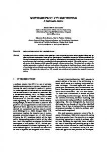
veloped that focus on defining the variability in systems and rely on other modeling languages to capture other system abstractions, e.g., requirements, architectural, or design models or even code [28]. A significant body of work exists on exploiting the unique features of software architecture abstractions for software validation, for example, detecting component mismatch [1], planning integration testing [3], and using notions of software architecture model coverage for test adequacy [29]. In contrast, there has been relatively little work on exploiting the unique features of software product line abstractions, namely the identification of commonality and variability, for validation. We contend that the key challenge for validation revealed at the product line layer of abstraction is the interaction between differing combinations of variability bindings. When using a product line, application developers make choices about how to bind capabilities to points of variability in their target system - also referred to as an instance of the product line. In this process, they must consider whether the combination of bindings they have chosen has ever appeared in an instance of the product line. If so, then they may have some confidence that interactions among the bound capabilities have been exercised, but if not, they may be wary of faults arising due to such interactions. Ideally, developers of software product lines would validate all possible combinations of capabilities and points of variability that can be realized in a product line instance. This would allow users to confidently instantiate the product line to produce new systems. Unfortunately, the space of possible combinations in a realistic product line is likely to be enormous and exhaustive consideration of those combinations intractable. In this paper, we address the problem of validating a software product line by defining families of coverage criteria for product line models. These criteria allow for tradeoffs to be made between the extent to which binding combinations are covered and the cost of testing. Furthermore, the criteria are related in such a way that developers of SPLs can exploit them to incrementally invest in improved validation across the lifetime of an SPL. It is important to emphasize that our work is focused on validation of the product line itself and not on specific instances of the product line, although we argue that the latter will be made more cost-effective by the former. Figure 1 illustrates the orthogonal dimensions of software product line coverage, and coverage of an instance of the product line, i.e., a program. Current approaches to testing SPLs in practice use well understood code coverage measures, for example, statement and branch coverage,

Software product line modeling has received a great deal of attention for its potential in fostering reuse of software artifacts across development phases. Research on the testing phase, has focused on identifying the potential for reuse of test cases across product line instances. While this offers potential reductions in test development effort for a given product line instance, it does not focus on and leverage the fundamental abstraction that is inherent in software product lines - variability. In this paper, we illustrate how rich software product line modeling notations can be mapped onto an underlying relational model that captures variability in the feasible product line instances. This relational model serves as the semantic basis for defining a family of coverage criteria for testing of a product line. These criteria make it possible to accumulate test coverage information for the product line itself over the course of multiple product line instance development efforts. Cumulative coverage, in turn, enables targeted testing efforts for new product line instances. We describe how combinatorial interaction testing methods can be applied to define test configurations that achieve a desired level of coverage and identify challenges to scaling such methods to large, complex software product lines.

1. INTRODUCTION A software product line (SPL) is a set of programs that share significant common functionality and structure. A product line is distinguished by the fact that the differences among the constituent programs is well-understood and is organized in some form. By explicitly capturing the variability among a set of programs, a software product line supports the systematic reuse of artifacts across the development activities for those programs. A number of authors have described the potential benefits that may accrue from using SPL techniques in the requirements, architecture, design, coding and testing phases [9, 15, 28]. Software product line modeling languages have been de-

Permission to make digital or hard copies of all or part of this work for personal or classroom use is granted without fee provided that copies are not made or distributed for profit or commercial advantage and that copies bear this notice and the full citation on the first page. To copy otherwise, to republish, to post on servers or to redistribute to lists, requires prior specific permission and/or a fee. ROSATEA ’06 July 17, 2006, Portland, Maine, USA Copyright 2006 ACM 1-59593-459-6/06/07 ...$5.00.

53

Instance Coverage

Partial Path

Branch

relational model. In Section 4 we leverage the relational model to define several coverage criteria and explain the concepts of cumulative coverage and targeted testing. Work in multiple areas of software modeling and validation has influenced our work; Section 5 describes those influences. Finally, in Section 6 we identify challenges to scaling existing testing techniques to treat large, complex software product lines cost-effectively.

2. BACKGROUND

Statement

A number of different modeling formalisms have been developed to capture different aspects of families of software products, e.g., [8, 13, 15, 28]. In this section, we provide an overview of one such formalism that we will use as a vehicle for formalizing and presenting SPL-specific test coverage and adequacy notions in Sections 3 and 4. We note, however, that our approach is applicable to a broad range of SPL modeling formalisms.

SPL Coverage Figure 1: SPL versus Instance Coverage

2.1 The Orthogonal Variability Model Pohl et al. introduce [7, 28] the Orthogonal Variability Model (OVM) to capture the commonality and variability within a product line. The OVM is intended to capture variability that cross-cuts a broad spectrum of software models defined in the UML. In this Section, we explain the elements of OVM as they relate to class diagram elements. Figure 2 illustrates an OVM model taken from [28] that captures a simple security system product line. There are two primary building blocks in OVM models. Variation points (VP) define the features of a system whose realization, or presence, may vary across product line instances; variation points are depicted as triangles. Variation points might correspond, for example, to an abstract class in a UML class diagram. Variants (V) correspond to a specific realization of a feature that may be bound to a variation point; variants are depicted as rectangles. A variant might, for example, correspond to a concrete class that implements the abstract class associated with a VP. A set of variants is related to a variation point through a variability dependency; a variability dependency is depicted as an edge connecting a triangle to a rectangle. Conceptually, a dependency captures the set of realizations of a feature that are possible in some instance of the product line. Variability dependence implies that variants may be bound to a variation point. The example in Figure 2 has 3 variation points and a total of 7 variants. OVM provides flexibility in defining dependencies. Mandatory dependencies, depicted as solid edges, require that a dependent variant be bound to a variation point in each PL instance that includes the VP; this can be thought of as a commonality at the level of abstraction captured by the OVM. Optional dependencies, depicted as dashed edges, allow for a variation point to be bound to the associated variant in a product line instance or not. If a variation point has multiple optional dependent variants, then it may be bound to a subset of those values. Finally, alternative choice dependencies allow for modelers to define the number of optional variants that may be bound with a variation point; these are depicted with a solid arc spanning a set of optional variability dependence edges. An alternative choice has upper and lower bounds defined on the size of the variant set. This is denoted [i, j] and means that the variation point has at least i and at most j variants bound to it in a product line in-

and focus on validation of the individual products generated from the SPL. While valuable, this approach provides for relatively low coverage of the space of possible SPL instances. Research in software testing focuses on developing techniques that more thoroughly sample a program’s behavior space based on consideration of implementation, design or architectural details. In this way, testing research is moving towards stronger notions of SPL instance coverage, for example, by using symbolic execution to generate tests that achieve partial path coverage. Our work seeks to define notions of SPL coverage and to develop techniques to sample the space of SPL instances to achieve different levels of coverage. The goal is to move practice towards a more thorough consideration of the variability space of an SPL. We note that ultimately one wants to achieve the highest degree of behavior and variability coverage of the product line, i.e., the upper right portion of Figure 1, for a given allocation of resources. To illustrate our approach to SPL coverage, we set our work in the context of an existing software product line modeling notation that has received significant recent attention Pohl et al.’s Orthogonal Variability Model (OVM) [28]. We map the OVM to a low-level relational model that makes explicit the semantics of OVM’s higher-level, and sometimes subtle, primitives. Coverage criteria are defined in terms of this relational model and subsumption relationships among the criteria are defined. We then describe how these criteria can form the basis for SPL lifecycle validation activities. Specifically, we introduce the concept of cumulative variability coverage which accumulates coverage information for an SPL across a series of product line instance development activities and which can be exploited to target testing activities for future product line instances. Our relational model allows application of interaction testing techniques, e.g., [10], to generate coverage adequate test sets for some of our criteria. We have identified limitations on the applicability of existing interaction testing techniques to SPL models that arise from the richness of SPL modeling notations, specifically the significant use of constraints. The next Section provides background on the OVM and on combinatorial interaction testing, which has significantly influenced our approach to defining coverage criteria. Section 2 details how OVM models are mapped onto a low-level

54

V

Camera Surveillance

VP

VP

VP

Intrusion Detection

Security Package

Door Locks

V

V

Motion Sensors

V

Cullet Detection

V

Basic

Advanced

V

V

Keypad

Fingerprint Scanner

requires_v_v requires_v_v

Figure 2: Example OVM Model [28] stance. All of the dependencies in Figure 2 are optional and there are three alternative choice groupings shown each with the, unwritten, default bounds of [1, 1]. The intrusion detection variation point has the most subtle dependencies. The alternative choice dependency covering the camera surveillance and motion sensors variants means that exactly one of those must be present in a product line instance. The optional dependence on the cullet detection variant means that it may also be present, but need not be. In complex product lines, it is often the case that multiple decisions about the binding of variants to variation points must be correlated. To support this, OVM allows the definition of multiple types of constraints, but in this presentation we focus on variant constraints which relate choices made about variants bound to different variation points. A requires variant constraint states that when a variation point is bound to a specified variant then a related variation point must be bound to a specified variant. The example in Figure 2 shows two such ternary constraints depicted as dotted edges. For example, whenever the basic security package variant appears in a product line instance, then the motion sensors and keypad variants must be bound to the intrusion detection and door locks variation points, respectively, in the instance. A complementary constraint, the excludes variant constraint states that when a variation point is bound to a specified variant then a related variation point must not be bound to a specified variant. Note that as defined, OVM constraints are binary, but it is trivial to define constraints between a variant and a set of variants by using multiple constraints. OVM allows constraints to be defined between bound variants and variation points and between pairs of variation points. For example, binding of a specific variant for a variation point may constrain an instance of the product line to require (exclude) another variation point. In this way, one can construct hierarchical relationships among variation points, where specific variant bindings trigger the inclusion of child variation points.

2.2

velop system tests that bind variation points to variants in combinations that correspond to what developers think will be common product line instances. Taking a broader view, we would need to test for all possible interactions between combinations of variants. For instance, it might turn out that when building the motion sensors module, the developer forgot to specify what happens when an exceptional value occurs that can only arise from the keypad, since the motion sensor was originally developed with the fingerprint scanner in mind. Figure 3 shows a view of the possible variants that can occur in combination with each other for this product line. The intrusion detection variation point must have either camera surveillance or motion sensors and may or may not have cullet detection. The security package must be either basic or advanced, while the door locks can use either a keypad or fingerprint scanner. In this model we have four columns, or factors, one for each variation point plus an additional factor to model the optional dependency for intrusion detection. Each of these factors has 2 possible values. The Cartesian product, CP , of this system has 24 = 16 elements representing the possible variant to variation point bindings. When planning a set of integration tests for this product line we should test each of the 16 combinations to find interaction faults. In this example the system is relatively small and it might be possible to test all 16 combinations, however this does not hold for long; a system with 20 factors, each with only three values, will result in 320 = 3, 486, 784, 401 combinations.

2.3 Covering Arrays The combinatorial nature of testing is well-understood and researchers have developed multiple techniques for treating the space of inputs to a program or configurations of a software system [5, 10, 17, 31]. Empirical evidence suggests that it is possible to systematically sample this space and test a subset of the tuples from CP [5, 10, 14, 21, 31]. Combinatorial interaction testing defines a subset size, t, of vectors from CP and guarantees that all possible t-tuples appear in a test at least once. A covering array, CA(N ; t, k, s) is an N × k array defined on s symbols, where S = (0, 1, . . . , s − 1), such that for any t-set of columns all ordered t − tuples from S occur at least once.

Testing A Product Line

Suppose we are planning to test the set of products defined by the example product line shown in Figure 2. For simplicity we will ignore the set of constraints. One might develop individual unit tests for the variants and then de-

55

Set of Product Instances Representing a CA(5;2,4,2)

Factors

Values

Intrusion Detection A

Intrusion Detection B

Security Package

Door Locks

Intrusion Detection A

Intrusion Detection B

Security Package

Door Locks

Camera Surveillance

None

Advanced

Fingerprint Scanner

Camera Surveillance

Cullet Detection

Basic

Keypad

Motion Sensors

Cullet Detection

Advanced

Fingerprint Scanner

Camera Surveillance

Cullet Detection

Advanced

Keypad

Motion Sensors

None

Advanced

Motion Sensors

None

Basic

Keypad

Camera Surveillance

Cullet Detection

Basic

Fingerprint Scanner

Figure 3: Model

Fingerprint Scanner

Example of Product Line Interaction

Figure 4: Model

Example of Product Line Interaction

Set of Product Instances Representing a VCA(8;2,4,2(CA(N;3,3,2))

This mathematical structure is used in statistical design of experiments [27] and has been applied to functional software testing [5, 10, 14, 21]. Typically the columns of the array are called “factors”, each of the factors has s “levels” or “values”, and t is the interaction strength, or simply the strength of the array; for consistency, we adopt this terminology in our work. A common strength of testing is t = 2, often called pair wise testing. In our product line example, we can select a set of product instances that represents a covering array. Figure 4 shows a set of product instances that make up a CA(5; 2, 4, 2). Careful inspection of the Figure reveals that this set of instances consists of all possible pairs of factor-value pairs from CP . For example, the pair of pairs (security package,advanced ) and (door locks,keypad ) appears in the third row. In [11, 12, 31], another type of a covering array called a variable strength array is described and used that allows finer control over the interaction space. It allows for different sizes of t for different subsets of factors. A product line developer may decide that certain variation points are more closely related or are more likely to interact. These can be tested with a higher strength of interaction coverage. More formally, a V CA(N ; t, k, s, C) is an N × k covering array, of strength t containing C, a vector of covering arrays each of strength > t, where each CA in C is defined on a subset of the k columns. In our example system, we could set t to be 2 for the whole system, and define t! = 3 for the three factors, intrusion detection A, intrusion detection B, and door locks. This means that all possible 3-tuples of these three factors must be included, while all possible pairs for the whole system will be included. Figure 5 shows a VCA for this system. Notice that the three way property does not necessarily hold for all of the factors (intrusion detection B, security package and door locks are missing some 3-tuples). A variable strength covering array can define multiple regions of higher interaction coverage even though we have shown only one. We have assumed in this example model that this is an unconstrained system. Covering arrays do not include a “natural” mechanism for describing constraints. In Table 4, there are some infeasible combinations given the set of constraints modeled in Figure 2. For example, the last tuple is invalid, because there is a constraint that requires: basic to occur with motion sensors and keypad. We discuss the implications of such constraints on interaction testing in Section 3.5.

Intrusion Detection A

Intrusion Detection B

Security Package

Door Locks

Camera Surveillance

None

Advanced

Fingerprint Scanner

Motion Sensors

Cullet Detection

Advanced

Fingerprint Scanner

Camera Surveillance

Cullet Detection

Advanced

Keypad

Motion Sensors

None

Basic

Keypad

Camera Surveillance

Cullet Detection

Basic

Fingerprint Scanner

Camera Surveillance

None

Basic

Keypad

Motion Sensors

Cullet Detection

Advanced

Keypad

Motion Sensors

None

Basic

Fingerprint Scanner

Figure 5: Example of Variable Strength Product Line Interaction Model

3. A RELATIONAL MODEL OF SPL VARIABILITY Product-line models are fundamentally relational and interaction testing exploits a relational encoding of possible system configurations. In this section, we describe how the OVM can be mapped onto a simple relational model that satisfies the requirements of interaction testing. Subsequently, in Section 4 we describe how this relational model can be exploited to support SPL testing.

3.1 A Simple Relational Model A domain is a finite set of values. A relation is a subset of a Cartesian product of some number of domains. We write domains as Di and a relation over k domains as Πki=1 Di where the Di need not be distinct. We say that such a relation has k factors. Elements of a relation are tuples. For a relation with k factors we will refer to elements as a k-tuple and write it as (v1 , . . . , vk ) where vi ∈ Di . We extract the value for a factor, i, from a tuple, t = (v1 , . . . , vk ), using a projection function, π(t, i) = vi where 1 ≤ i ≤ k. We lift this function to sets of factors, {i, . . .}, to produce a tuple of values, π(t, {i, . . .}) = (vi , . . .), one for each factor.

3.2 Basic OVM Mapping Our goal is to construct the definition of a relation that encodes exactly the set of product line instances captured by an OVM model. In this way, our relational model makes explicit the semantics of OVM. We achieve this by defining a base relation that over approximates the set of product

56

VP

VP

OneOr Two

AtMost One

[1,2]

V

A

of the three variants could be selected. DOneOrTwo1 = {vA , vB , vC } models the fact that at least one variant must be bound, whereas DOneOrTwo2 = {vA , vB , vC , %} models the fact that a second variant may be bound. The constraint OneOrTwo1 &= OneOrTwo2 is required. For the AtMostOne variation point in Figure 3.2 an explicit bound of [0, 1] is defined. Consequently, one factor would be used to model the possibility that one of the two variants could be selected. DAtMostOne1 = {vA , vB , %} models the fact that at least one variant may be bound, and, as in the above example no constraint is needed for the single factor. In the worst case, where all dependencies are optional, an OVM model with k variants will give rise to a relational model with k factors. We note, however, that alternative choices with default [1, 1] bounds seem to be very common in OVM models [28]. Given this, we have optimized our mapping of the default alternative choice so that it uses a single factor and no constraints. Consequently, in practice, we expect the number of factors in our relational models to be closer to the number of variation points than to the number of variants.

[0,1]

V

B

V

C

V

A

V

B

Figure 6: Alternative Choice Examples

line instances and then successively restrict that relation. A variation point is modeled by a set of factors and variants are modeled as values. Variability dependencies relate a set of variants to a variation point, consequently, in our model the domain for a variation point’s factors are defined in terms of the set of values for the associated variants. For the example in Figure 2, we define a door locks factor over a domain that includes the values keypad and fingerprint scanner. Mandatory dependencies require that a variant be bound to the variation point in each product line instance, hence, this relation is invariant across the product line and we do not include it in the relational model. Optional dependencies, on the other hand, allow a variation point to be related to a set of associated variants. This is modeled by introducing a factor for each optional variant of the variation point that is defined over the domain comprised of the variant value and an additional value corresponding to no variant, denoted %; we denote the set of factors for a variation point vp as f (vp). To illustrate in terms of the example in Figure 2, consider the situation of the door locks variation point if the associated dependences were not covered by an alternative choice, i.e., if there were simply two optional dependences. We would define factor door-locks1 over Ddoor-locks1 = {vkeypad , %} and factor door locks2 over Ddoor-locks2 = {vf ingerprintscanner , %}. Alternative choice dependencies introduce additional complexity since they define bounds on the number of variants that can be related to a variation point. An alternative choice with bounds [i, j] is modeled with: (1) i factors for the variation point with a domain defined by the exact set of variant values covered by the alternative choice, and (2) j −i factors for the variation point with a domain defined by the set of variant values covered by the alternative choice and %. Furthermore, we introduce inequality constraints between all such pairs of factors to enforce the fact that a variation point can be bound to a variant only once; technically we only require inequality for non-% values. Since the semantics of alternative choice can be somewhat subtle we present a series of three examples to illustrate our mapping. The alternative choice for door locks in Figure 2 has the default bounds of [1, 1], thus only a single factor is used to model the fact that exactly 1 variant is chosen: Ddoor-locks = {vkeypad , vf ingerprintscanner }. With a single factor in this case, no inequality constraints are needed. For the OneOrTwo variation point in Figure 3.2 an explicit bound of [1, 2] is defined. Consequently, two factors would be used to model the possibility that two out

3.3 Mapping OVM Constraints Thus far, we have not considered explicit OVM constraints. If we ignore the inequality constraints introduced above, we have a relation, for a given OVM model, U = Πvp∈OV M Πf ∈f (vp) Df that we refer to as the unconstrained model. Tuples of the unconstrained model over approximate potential product line instances - the model includes all possible product line instances, but it may include instances that are inconsistent with inequality and OVM constraints. Our strategy for incorporating constraints is to define subrelations of U that are consistent with each constraint and then intersect the resulting constraints. An inequality constraint between factors i and j is defined as: I(i, j) =

{t | t ∈ U ∧ (π(t, i) &= % ⇒ π(t, i) &= π(t, j))}

The cumulative constraint for a variation point, vp, is I(vp) =

\

I(i, j)

i∈f (vp),j∈f (vp)−{i}

and for an OVM model: I=

\

I(vp)

vp∈OV M

Explicit constraints in OVM are used to restrict instances of the product line from including certain combinations of variants and variation points. We first consider variant to variant constraints, depicted graphically with ..._v_v annotations. A requires variant to variant constraint states that when a designated variation point is bound to a specific variant then another variation point must be bound to a specific variant. As above, we model the constraint by defining a sub-relation of U whose tuples are all consistent with the constraint. Let i and j be the two variation points and v and w be the values associated with the variants, then

57

the requires variant constraint is defined as: R(i, v, j, w)

=

The covering array property, that all t-tuples must occur in any arbitrary t columns can S be expressed as follows in the relational model. Let F = vp∈OV M f (vp) be the set of all factors in a relational model. For all S ⊆ F ∧ |S| = t let RTS = Πf ∈S Df be the indexed set of all pairs of values over the t-size subset of factors, S. For N to be a t-way covering array it must be the case that

{t | t ∈ U ∧ (∃f ∈f (i) : π(t, f ) = v) ∧ (∃f ∈f (j) : π(t, f ) = w)} ∪ {t | t ∈ U ∧ (∀f ∈f (i) : π(t, f ) &= v)}

An excludes variant to variant constraint serves a similar, but complementary, function in OVM models and is defined as: E(i, v, j, w) =

∀S⊆F ∧|S|=t : ∀ts ∈RTS : ∃t∈N π(t, S) = ts

{t | t ∈ U ∧ (∃f ∈f (i) : π(t, f ) = v) ∧ (∀f ∈f (j) : π(t, f ) &= w)} ∪

Informally, this means that all possible t-sized tuples must be embedded in some full-tuple in N . In Section 2.3 we presented a model of software product line t-way interactions using covering arrays. We avoided a discussion of constraints, however. Suppose we use the constraint from Figure 2 that basic requires motion sensors and keypad and tighten it by stating that basic excludes cullet detection. This invalidates the last line of Figure 4 as part of the SPL. It turns out that this is a relatively easy constraint to handle in the system; we simply remove the last product instance of the covering array. All of the other pairs in that instance, such as camera surveillance and fingerprint scanner are already covered in other product instances; Figure 7 shows an example of this scenario. Suppose,instead, we impose a different constraint, namely that camera surveillance requires fingerprint scanner (see Figure 8). The third product instance is now invalid. However, unlike the previous scenario, we cannot simply remove this instance. Other pairs in this product instance, such as advanced and keypad are not covered elsewhere. If we alter other instances to account for these, then we lose other required tuples. There is no way to satisfy this constraint without adding another product instance back into this set. We have increased redundancy among other product variants, but this is necessary to include all possible pairs of feasible interactions. Adding multiple constraints, can complicate building a legal subset of product instances that satisfy the covering array properties. Some work has addressed these types of issues [6, 10, 18] however, no cost-effective techniques for handling multiple and complex constraints in interaction test generation are known at present.

{t | t ∈ U ∧ (∀f ∈f (i) : π(t, f ) &= v)}

OVM also supports variant to variation point and variation point to variation point constraints, depicted graphically with ..._v_vp and ..._vp_vp annotations. A requires variation point to variation point constraint states that when a designated variation point is bound to some variant then another variation point must be bound to some variant, i.e., it cannot be unbound, in a product line instance. It’s definition is similar the variant to variant requires constraint. Let i and j be the two variation points, then the requires variant constraint is defined as: R(i, j)

=

{t | t ∈ U ∧ (∃f ∈f (i) : π(t, f ) &= %) ∧ (∃f ∈f (j) : π(t, f ) &= %)} ∪

{t | t ∈ U ∧ (∀f ∈f (i) : π(t, f ) = %)}

Excludes variation point to variation point constraints are defined similarly. Variant to variation point constraints are defined as a hybrid of variant to variant and variation point to variation point definitions. The constraints defined above are all 1-1, but OVM’s graphical notation permits the definition of 1-many constraints, for example, in Figure 2, the dotted hyper-edge from basic to motion sensors and keypad. 1-many constraints are syntactic sugar for the intersection of a collection of 1-1 constraints; consequently our mapping to the relational model simply desugars them.

3.4

Combining Relational Models

We have defined all of our constraints as sub-relations of U , thus constraints can be enforced by simply intersecting them with U . We refer to a model that intersects U with some set of constraint relations a constrained model. The conjunction of all constraints for an OVM model: \ \ U ∩I ∩ R(. . .) ∩ E(. . .)

Constrained Set of Product Instances “Basic requires Motion Sensors and Keypad” “Basic Excludes Cullet Detection” Intrusion Detection A

Intrusion Detection B

Security Package

Door Locks

Camera Surveillance

None

Advanced

Fingerprint Scanner

Motion Sensors

Cullet Detection

Advanced

Fingerprint Scanner

is called the feasible model and it contains the exact set of product line instances derivable from the OVM model.

Camera Surveillance

Cullet Detection

Advanced

Keypad

Motion Sensors

None

Basic

Keypad

3.5 Relational Model as a Covering Array

Camera Surveillance

Cullet Detection

Basic

Fingerprint Scanner

Some selections of N product instances where N ⊆ U can be mapped to a covering array. We map our relational model to a (potential) covering array as follows. Each product instance is a full-tuple of the relational model, i.e., a tuple that includes all factors, which becomes a single row of the covering array. A factor in the relational model is a factor (or column) in the covering array. The cardinality of Di in the relational model equals s in the covering array model 1 .

Figure 7: Constraint Reduces the Set of Product Instances

4. SPL TEST COVERAGE AND ADEQUACY In practice, the space of feasible product line instances may be enormous and it will be intractable to test all of them. Consequently, we adopt, for SPL testing, the same strategy taken with other coverage notions - we relax the

1

A more general case of the covering array exists that we have not discussed here, that will handle differing numbers of values for each domain.

58

{C1,C2,…,Ck}

Constrained Set of Product Instances “Camera Surveillance requires Fingerprint Scanner” Intrusion Detection A

Intrusion Detection B

Security Package

Door Locks

Camera Surveillance

None

Advanced

Fingerprint Scanner

Motion Sensors

Cullet Detection

Advanced

Fingerprint Scanner

Camera Surveillance

Cullet Detection

Advanced

Keypad

Motion Sensors

None

Basic

Keypad

Camera Surveillance

Cullet Detection

Basic

Fingerprint Scanner

Motion Sensors

Cullet Detection

Advanced

Keypad

{C2,…,Ck}

U

{Ck} {}

Figure 8: Constraint Does Not Reduce the Set of Product Instances

!

!

!i=1..k Ci !i=2..k Ci

U

!

Ck U

Figure 9: Subsumption of Constraint-sensitive Coverage Criteria

coverage criteria to consider only a portion of the feasible system behavior. The relational model of SPL variability developed in the previous section reveals multiple dimensions in which such relaxations can proceed. In the remainder of this section, we outline two families of test adequacy criteria based on partial coverage of SPL variability, and then describe how to exploit coverage notions for SPL testing.

4.1

U

to generate an adequate test set using combinatorial interaction methods. Since constraint-sensitive and interaction strength criteria are orthogonal, it is possible to combine them and, in fact, the traditional approach to interaction testing described in Section 2 achieves a combination of unconstrained 2-way coverage. Closely related to the interaction strength criteria are the variable strength criteria which allow the factors in a model to be partitioned into sets of potentially different sizes and require all combinations of values to be covered within each set. As defined in [11], variable strength coverage may involve a large number of different strengths focusing on different sets of factors. We identify the minimal, i, and maximal, j, strengths in a variable strength cover and refer to it as [i, j]-way; note that multiple distinct variable strength covering arrays may be mapped to the same [i, j]-way designation. Given the large number of sub-groupings and sizes possible in a variable strength cover, we do not attempt to define a subsumption hierarchy for these criteria, except for the trivial situation where [i, j]-way subsumes [i! , j ! ]-way coverage if i ≥ j ! . We can however, define their relationship to interaction strength criteria: [i, j]-way coverage subsumes i-way coverage and j-way coverage subsumes [i, j]-way coverage.

Test Adequacy Criteria

The relational model of SPL variability is constructed by intersecting sets of constraints with the unconstrained model. This gives rise to a family of constraint-sensitive criteria that vary in terms of the set of constraints they include. Let C be the set of all constraints. Then the the lattice formed by P(C) and ⊆ defines a set of coverage criteria varying in their precision. An element T S ∈ P(C) is a set of constraints that define a criteria U ∩ s∈S s. For the bottom element of the lattice, the empty set of constraints, we define the criteria as U , and for the top element the criteria is the feasible model. While the lattice is ordered by ⊆, we note that the criteria defined by lattice points are ordered by ⊇, since adding additional constraints makes the resulting relation no larger. A criteria higher in this order subsumes one lower in the order, since achieving tuple-coverage of the former guarantees it of the latter. Figure 9 illustrates a chain in the lattice and it’s subsumption relationships. This family of criteria may give rise to significant differences in the cost of generating adequate test sets using combinatorial interaction methods, since they do not cope well with highly constrained relations. Constraint-sensitive criteria as defined above, still consider the full-tuple of all variation point related factors. By considering tuples of smaller size we can define a family of interaction strength criteria that are ordered by the number of factors that are included in the tuples, i.e., the strength of factor interaction. A related set of coverage criteria was presented in [16], we extend and refine several of those criteria to better adapt them to SPL models. For example, coverage at strength 2, requires all pairs of factors to take on all possible values. Let k be the total number of factors in the relational model, then (i + 1)-way coverage subsumes i-way coverage for 0 ≤ i < k since each tuple of size i is embedded in some tuple of size i + 1. Since these criteria are exhaustive, they are sensitive only to the number of factors not the identity of the factors. As with constraint-sensitive criteria, interaction strength criteria can vary widely in the cost

4.2 Cumulative Test Coverage For a large SPL, it may be very expensive to perform adequate testing relative to the criteria outlined above. We expect that the lifespan of a software product line, i.e., the time span over which new instances of the SPL are produced, will be significantly longer than the development time of a single instance of the product line. We believe that the long lifespan of an SPL provides an opportunity to perform validation activities whose cost would be prohibitive for a single program, but when amortized over a set of SPL instances would be considered cost-effective. Intuitively, one is interested in assuring a desired level of coverage of the portion of an SPL that is related to a specific instance at the time when that instance is to be produced. Achieving coverage of an instance before it is to be produced may be desirable, but only if time and resource constraints permit. Delaying coverage until after an instance is released risks inadequate testing. Given the lifespan of an SPL and the fact that the development of SPL instances will be ordered in time, we be-

59

time

process seeks to incrementally increase the CVC. One way to achieve this is to generate instances of the SPL for the express purpose of validation - as opposed to deploying those instances. Consider a situation where there are 100 2-way binding combinations possible, and 78 of those have been covered already by previous product line instance testing. We could generate a set of product line instances that cover the 22 remaining binding combinations to produce a CVC that is 2-way adequate for the product line as a whole; Figure 10 illustrates the generation of n test instances, testinstance 1 . . . test-instance n , for this purpose. We emphasize that the problem of testing the individual instances and the degree of coverage demanded in instance testing is an important, but orthogonal, dimension of testing SPLs. In product line instance development efforts, for example, instance5 in Figure 10, developers may determine, for instance, that the CVC is 2-way adequate and then shift their focus to higher-strength criteria. They might, for example, assess the 3-way coverage in the CVC relative to the instance being developed. Imagine that one triple of variability bindings in the instance is uncovered in the CVC. The developer may use that combination to drive the development of tests that are targeted to exposing interactions among the portions of the implementation that realize those three variability bindings. In this way, the instance testing effort would be focused based on the results of the overall SPL validation effort.

SPL Validation Phase test-instance1 test-instance2 .. . test-instancen

instance1 instance2 instance3 instance4

Instance Development Phase instance5

SPL Deployed

Current Time

Figure 10: Cumulative Coverage Over an SPL Lifespan

lieve that one should stage the process of achieving a desired level of SPL coverage. Figure 10 illustrates an SPL deployment scenario. Four instances of the SPL have been produced, two of which are still deployed at the current time. The instance-specific testing for each of these yields coverage information about the combinations of variants in the instance. In particular, this coverage information, denoted vc(i) for instancei , includes sets of pairs, triples, etc., all the way up to a single k-way tuple defining the full set of variability bindings in the instance. We refer to the variability coverage achieved at a specific time, t, in the lifespan of an SPL,Ss, as its cumulative variability coverage (CVC), cvct (s) = 0≤i≤n vc(i) where n is number of instances produced from s prior to t. One can consult the CVC to calculate the percentage of all feasible variability combinations of a given arity that have been covered. Developers will view the sequence of interaction strength coverage percentages to develop an overall picture of the current state of SPL validation. Given the subsumption relationship between different interaction strength criteria the coverage percentages for increasing strengths will be non-increasing, e.g., the percentage of pair-wise coverage will be greater or equal to the percentage for three-way coverage.

4.3

5. RELATED WORK An enormous body of work on coverage criteria and notions of test adequacy has been reported in the literature. We will not survey it here. Instead we remark that a number of researchers have considered exploiting software architecture models to drive the planning, generation, and assessment of software testing. Many of the ideas in this space can be traced back to Richardson and Wolf [29], but the most mature development of architecture-based testing is the work of Muccini et al. [24]. These methods exploit both structural and behavioral information captured in architecture descriptions. SPL models add the dimension of variability which these approaches do not address, but which we treat explicitly in our work. We note that a complete approach to testing will likely take into account notions of coverage derived from product line variability, and architectural descriptions as well as other sources of information about the software system being validated. The work of Grindal et al. [16] presents a subsumption hierarchy of coverage for a wide range of “combination testing” methods which includes interaction testing as represented by covering arrays. In our subsumption we differ by only including subsumption rules for the covering array interaction model. We modify and collapse some of their layers, re-define where variable strength arrays fit into the model and address the issue of constraints. Williams and Probert [30] also present a model for interaction test coverage but this is a simple model that does not include subsumption or constraints. Several researchers have considered the unique challenges of testing SPLs. Muccini and van der Hoek [25] provide an overview of many of the issues. They mention the large space of variability combinations as a key challenge, but do not propose test coverage approaches that allow for costeffectiveness tradeoffs as we do. They describe how testing

Targeted Testing

During SPL development and deployment we envision an alternation between phases that emphasize overall SPL validation and SPL instance development. The CVC provides a means for driving and assessing the former and for focusing the latter to achieve greater coverage than would be cost-effective in a single program development effort. Specifically, we envision that the cumulative variability coverage will enable three advantages for product line developers: (1) coverage percentages for different interaction strengths will provide an overall metric of SPL quality, (2) the extent to which the variability combinations in a specific product line instance are contained in the CVC indicates how thoroughly the SPL has been validated with respect to that instance, and (3) variability binding combinations in an SPL instance that are not covered in the CVC can be used to drive testing of that instance. These advantages are increased if the SPL development

60

constructing covering arrays. They do not explicitly model constraints between factors and their values (they call these side constraints), but rather mention them as future work. Hartman and Raskin [18] briefly discuss the existence of covering array constraints, but require that they be expressed by enumerating all infeasible k−tuples. They do not discuss the implication on coverage criteria.

might be targeted at portions of new product line instances that have yet to be considered, but they do not propose a framework for cumulative test coverage that will enable targeted testing. PLUTO [4] is a methodology that has the same goal as our work - identifying the bindings of variability points in an SPL that should be tested. Their method is largely manual, based on category partition techniques [26], whereas ours exploits automated combinatorial interaction techniques. While they do not propose coverage or test adequacy criteria, they do expose the fundamental role that constraints play in generating SPL tests. The RITA project is focused on providing tool support for product family development. Much of their focus is on artifact reuse, but they have also considered the development of customized notions of coverage and adequacy that are appropriate for restricted classes of SPLs [20]. The work of McGregor is the most closely related to ours in that it considers the connection between combinatorial interaction methods, in his case orthogonal arrays, to covering the space of SPL variability points [23]. He does not, however, provide details on how SPL models such as OVM, can be mapped onto appropriate representations to allow interaction methods to be applied, nor does he address the significant challenges arising from the use of constraints in those models, and finally he does not develop the connection between interaction methods and test coverage criteria. We considered the OVM model in this paper and the developers of OVM suggest three strategies for testing software product lines [7, 28]: brute force which corresponds to coverage of all tuples in our feasible model, pure application which corresponds to covering individual tuples corresponding to product line instances that are produced, and sample application which corresponds to sampling tuples from our feasible model. Our approach is considered a sampling technique. The brute force and pure application strategies can be seen as endpoints of the spectrum of full-tuple approaches, but as discussed in Section 4, there are multiple dimensions of coverage that may be varied to trade off the cost of generating and running tests of SPL instances with SPL coverage. Finally our work can be seen as the application and customization of ideas from interaction testing to SPLs. There is a long history of research on interaction testing of which we only briefly summarize some highlights. Mandl [22] was the first to recognize the power of combinatorial designs (he used a related structure, mutually orthogonal latin squares) for use in software testing. He applied his technique to test enumerated types in an Ada compiler. Brownlie, et al. developed the orthogonal array test generator (OATS) at AT&T [5]. Orthogonal arrays are a specialized form of a covering array. D. Cohen et al. [10] suggest the use of covering arrays as a model of interaction testing. They also discuss a simple constraint handling mechanism. All three of these studies presented empirical evidence that interaction testing with t = 2 adds value. Additional empirical evidence of use on covering arrays extends their work to higher interaction strengths [14, 21, 31]. There has also been a large body of mathematical work on the construction of covering arrays. A survey on this topic is presented by Hartman in [17]. Most of this work does not explicitly handle constraints. In [19], Hnich et al. present constraint handling techniques for modeling and

6. CHALLENGES AND FUTURE WORK We have defined a relational model for software product lines that provides a set of adequacy and coverage criteria across a family of products. It takes into consideration the variability and constraints in SPLs and maps directly onto a known combinatorial testing method. Although this provides us with a viable approach to support the testing of product lines, it remains preliminary work. We conclude with a list of challenges that must be addressed as the next steps in refining our work. Scalability The OVM model presented in Figure 2 represents a small fragment of a software product line. Scaling our approach to cost-effectively treat the size and complexity of SPL models that arise from real systems is a significant challenge. Clearly the use of sampling through covering arrays for testing product instances will help reduce the overall test space, and will, thereby, provide collection of low-cost test adequacy criteria. The extent to which less precise criteria provide for effective SPL testing, however, remains a question. Rich Constraints As constraints grow in complexity and number, the difficulty of modeling and generating covering test sets for product lines increases. We believe that constraints should only be used to express the semantics of variability combinations in an SPL. It may well be the case that developers use constraints to describe the currently planned instances, rather than the possible instances, in order to manage the size of the test space; this is common practice when using TSL [26]. This should be avoided since it unnecessarily interferes with the ability of automated test coverage techniques to scale to larger systems. In many situations, large numbers of complex constraints may well be needed. We need to understand the structure and inter-relationship of these constraints in order to develop effective techniques for extending existing interaction testing methods to treat constraints. Unbounded Models Recent work [2, 13] has proposed the use of context-free grammars and unbounded cardinality constraints in feature modeling. These render our relational modeling scheme unworkable, since it is defined based on a known fixed number of factors. One possible approach is to apply our technique to a bounded set of SPL instances generated from such an unbounded model. Evolution Another aspect of product lines that make them difficult to model with our relational approach is that of evolution. Inherent in the product line definition is the idea that a product line will evolve and grow. While models like the OVM do not directly account

61

for evolution other researchers have considered the issue. For example, certain forms of evolution, such as specialization [13], are easily detected and accommodated in our approach, where as other forms, such as extension with a new variant, would require some form of feature model impact analysis and modification of CVC information.

[8]

[9]

Empirical Evidence and Benchmarks The empirical evidence that interaction testing may be valuable comes from the mainstream software testing community. Empirical evidence on real software product lines is clearly needed to understand their size (i.e. numbers of variation points and variants), the extent and complexity of constraints, and the effectiveness and feasibility of combinatorial testing methods.

[10]

[11]

This requires, of course, access to realistic SPL models and artifacts. We believe that the academic and industrial research communities interested in product line development would benefit greatly from the availability of a collection of benchmark software product lines. Academia would have non-trivial subjects to use in empirical studies, and industry would be able to judge the applicability of emerging research results since those results would have been evaluated on wellunderstood systems that share properties with those in industry.

[12]

[13]

[14]

7. ACKNOWLEDGMENTS This work was supported in part by NSF CCF through awards 0429149 and 0444167, by the U.S. Army Research Office through award DAAD190110564 and by an NSF EPSCoR FIRST award. We would like to thank John Hatcliff for discussions about modeling and analysis of constraints in software product lines.

[15]

[16]

8. REFERENCES [1] R. Allen and D. Garlan. A formal basis for architectural connection. ACM Transactions on Software Engineering and Methodology, 6(3):213–249, 1997. [2] D. Batory. Feature models, grammars, and propositional formulas. In Proceedings of the International Conference on Software Product Lines, pages 7–20, Oct. 2005. LNCS 3714. [3] A. Bertolino, F. Corradini, P. Inverardi, and H. Muccini. Deriving test plans from architectural descriptions. In Proceedings of the International Conference on Software Engineering, pages 220–229, 2000. [4] A. Bertolino and S. Gnesi. Use case-based testing of product lines. In Proceedings of the European Software Engineering Conference, pages 355–358, 2003. [5] R. Brownlie, J. Prowse, and M. S. Phadke. Robust testing of AT&T PMX/StarMAIL using OATS. AT& T Technical Journal, 71(3):41–47, 1992. [6] R. Bryce and C. Colbourn. Prioritized interaction testing for pairwise coverage with seeding and constraints. Journal of Information Science and Technology. To appear. [7] S. B¨ uhne, K. Lauenroth, and K. Pohl. Modelling requirements variability across product lines. In

[17]

[18]

[19]

[20]

[21]

[22]

62

Proceedings of the International Conference on Requirements Engineering, pages 41–50, August 2005. A. Childs, J. Greenwald, G. Jung, M. Hoosier, and J. Hatcliff. Calm and cadena: Metamodeling for component-based product-line development. IEEE Computer, 39(2), 2006. P. Clements and L. M. Northrop. Software Product Lines: Practices and Patterns. Addison Wesley, 2001. D. M. Cohen, S. R. Dalal, M. L. Fredman, and G. C. Patton. The AETG system: an approach to testing based on combinatorial design. IEEE Transactions on Software Engineering, 23(7):437–444, 1997. M. B. Cohen, C. J. Colbourn, J. Collofello, P. B. Gibbons, and W. B. Mugridge. Variable strength interaction testing of components. In Proceedings of the International Computer Software and Applications Conference, pages 413–418, 2003. M. B. Cohen, C. J. Colbourn, P. B. Gibbons, and W. B. Mugridge. Constructing test suites for interaction testing. In Proceedings of the International Conference on Software Engineering, pages 38–48, May 2003. K. Czarnecki, S. Helson, and U. Eisenecker. Fromalizing cardinality-based feature models and their specialization. Software Process : Improvement and Practice, 10(1):7–29, 2005. I. S. Dunietz, W. K. Ehrlich, B. D. Szablak, C. L. Mallows, and A. Iannino. Applying design of experiments to software testing. In Proceedings of the International Conference on Software Engineering, pages 205–215, 1997. H. Gomaa. Designing Software Product Lines with UML : From Use Cases to Pattern-based Software Architectures. Addison Wesley, 2004. M. Grindal, J. Offutt, and S. F. Andler. Combination testing strategies: a survey. Software Testing, Verification and Reliability, 15(3):167–199, 2005. A. Hartman. Software and hardware testing using combinatorial covering suites. In Graph Theory, Combinatorics and Algorithms: Interdisciplinary Applications, pages 327–266, 2005. A. Hartman and L. Raskin. Problems and algorithms for covering arrays. Discrete Math, 284:149 – 156, 2004. B. Hnich, S. Prestwich, and E. Selensky. Constraint-based approaches to the covering test problem. Lecture Notes in Computer Science, 3419:172–186, March 2005. R. Kauppinen, J. Taina, and A. Tevanlinna. Hook and template coverage criteria for testing framework-based software product families. In Proceedings of the International Workshop on Software Product Line Testing, pages 7–12, August 2004. D. Kuhn, D. R. Wallace, and A. M. Gallo. Software fault interactions and implications for software testing. IEEE Transactions on Software Engineering, 30(6):418–421, 2004. R. Mandl. Orthogonal latin squares: An application of experiment design to compiler testing. Communications of the ACM, 28(10):1054–1058, October 1985.

[23] J. D. McGregor. Testing a software product line. Technical report, Carnegie Mellon, Software Engineering Institute, December 2001. [24] H. Muccini, A. Bertolino, and P. Inverardi. Using software architecture for code testing. IEEE Transactions on Software Engineering, 30(3):160–171, 2004. [25] H. Muccini and A. van der Hoek. Towards testing product line architectures. In Proceedings of the International Workshop on Test and Analysis of Component-Based Systems, 2003. [26] T. J. Ostrand and M. J. Balcer. The category-partition method for specifying and generating functional tests. Communications of the ACM, 31(6):676–686, 1988. [27] M. S. Phadke. Quality Engineering Using Robust Design. Prentice-Hall, Inc., New Jersey, 1989. [28] K. Pohl, G. B¨ ockle, and F. van der Linden. Software Product Line Engineering. Springer, Berlin, 2005. [29] D. J. Richardson and A. L. Wolf. Software testing at the architectural level. In Joint proceedings of the International Software Architecture Workshop and International Workshop on Multiple Perspectives in Software Development, pages 68–71, 1996. [30] A. W. Williams and R. L. Probert. A measure for component interaction test coverage. In Proceedings of the ACS/IEEE International Conference on Computer Systems and Applications, pages 301–311, 2001. [31] C. Yilmaz, M. B. Cohen, and A. Porter. Covering arrays for efficient fault characterization in complex configuration spaces. IEEE Transactions on Software Engineering, 31(1):20–34, 2006.

63