Apr 17, 2007 - Matrix-exponential distribution, Coxian distribution, phase-type distri- ... Neuts [22] introduced the PH-distribution as the distribution of the ...
Coxian Approximations of Matrix-Exponential Distributions Qi-Ming He∗ and Hanqin Zhang† April 17, 2007
Abstract In this paper, we study the approximation of matrix-exponential distributions by Coxian distributions. Based on the spectral polynomial algorithm, we develop an algorithm for computing Coxian representations of Coxian distributions that are approximations of matrix-exponential distributions. As a specialization, we show that phase-type (PH) distributions can be approximated by Coxian distributions. We also show that any phase-type generator with only real eigenvalues is PH-majorized by some ordered Coxian generators. Consequently, the algorithm is modified for computing ordered Coxian representations of any phase-type distribution whose Laplace-Stieltjes transform has only real poles. Numerical examples are presented to show the efficiency of the algorithm and the accuracy of the Coxian approximations. Key words. Matrix-exponential distribution, Coxian distribution, phase-type distribution, matrix analytic methods, Perron-Frobenius theory. Mathematics subject classification. Primary 60A99, Secondary 15A18.
∗
Department of Industrial Engineering, Dalhousie University, Halifax, N.S., Canada B3J 2X4. † Institute of Applied Mathematics, Academy of Mathematics and Systems Science, Academia Sinica, Beijing, 100080, China.
1
1
Introduction
This paper focuses on the approximation of matrix-exponential (ME) distributions by Coxian distributions. An algorithm is developed for computing Coxian representations of Coxian approximations of ME-distributions. As a specialization, the problem of Coxian approximations of phase-type (PH) distributions is resolved. Moreover, the algorithm developed in this paper is modified for computing ordered Coxian representations for PH-distributions whose Laplace-Stieltjes transform has only real poles. Neuts [22] introduced the PH-distribution as the distribution of the absorption time of a finite-state Markov process. Since the class of PH-distributions is dense in the class of all probability distributions with nonnegative support, the introduction of PH-distributions made it possible to study complicated queueing models such as the P H/P H/c queue analytically and numerically (Takahashi [33]). ME-distributions are generalizations of PHdistributions and have been used in the study of queueing models (Lipsky [19]). Asmussen and Bladt [4] studied ME-distributions and their corresponding renewal processes and queueing models. Today, both PH-distributions and ME-distributions have been widely used in the study of queueing networks, reliability models, supply chain models, insurance and risk models, and telecommunications systems (Asmussen [2, 3], Latouche and Ramaswami [18], Neuts [23, 24], and references therein). It is well known that the representation of a PH-distribution is not unique. To reduce the time complexity of algorithms involving PH-distributions, it is useful to find representations with the minimal number of phases. This is known as the minimal PH-representation problem (Commault and Mocanu [7], Mocanu and Commault [21], Neuts [22, 25], O’Cinneide [26, 27, 28, 29, 30]). Commault and Mocanu [7] and O’Cinneide [30] reviewed the literature on PH-distributions in recent years. While the problem of finding the minimal PH-representation of a PH-distribution is still open, the problem of finding simpler representations for PH-distributions or other probability distributions has been investigated extensively in recent years ([4, 7, 10, 11, 21, 26, 27, 28, 29]) with the focus on finding PHrepresentations with a simple structure for PH-distributions that approximate probability distributions (Altiok [1], Asmussen [2], and Bobbio, Horv´ath, Scarpa, and Telek [6]). The Coxian representation is one of the simpler PH-representations that have been investigated (Cumani [10], Dehon and Latouche [11], and O’Cinneide [26, 28, 29]). Erlang [12] introduced the idea of phase into the study of telephone systems, which led to the introduction of Erlang distributions in probability and statistics. Cox [8, 9] generalized the class of Erlang distributions and systematically studied probability distributions as mixtures of Erlang distributions. Consequently, Cox [8, 9] gave the first definition of Coxian distributions that have been used in many branches of science and engineering. In O’Cinneide [28], it was shown that Coxian distributions with a positive density function on 2
positive real numbers have an ordered Coxian representation, which is a special bi-diagonal PH-representation. Coxian representations have many advantages in numerical computations. For instance, the eigenvalues of their Coxian generators are the diagonal elements and can be used directly without further numerical computation. Therefore, it is computationally attractive to replace ME-representations or PH-representations with Coxian representations in the study of stochastic models. For that purpose, we need to find Coxian representations of Coxian distributions that approximate ME-distributions or PH-distributions. The objective of this paper is to introduce an algorithm for computing Coxian representations of Coxian distributions as approximations of ME-distributions and PH-distributions. Recently, HE and Zhang [15] (also see HE and Zhang [14, 16]) developed a spectral polynomial approach for computing bi-diagonal representations of PH-distributions. The idea of the spectral polynomial approach is to treat a PH-generator as a linear mapping and to generate some invariant polytopes of that linear mapping in order to calculate new MErepresentations. The theory developed in [15] provided the basis for developing an algorithm for computing Coxian representations and Coxian approximations. In HE and Zhang [16], based on the spectral polynomial approach, an algorithm for computing minimal Coxian representations for Coxian distributions was developed. The algorithm in HE and Zhang [16] dealt with individual Coxian distributions, while the algorithm in this paper focuses on PH-generators. Thus, the algorithm developed in [16] complements the algorithm of this paper. In van de Liefvoort and Heindl [34], computational methods were developed for evaluating ME-distributions with a given representation. That paper considered the numerical evaluation of ME-distributions, while this paper finds Coxian representations of Coxian approximations of ME-distributions. In this paper, we first concentrate on the class of ME-distributions and develop an algorithm that can be used to find some special Coxian distributions as approximations of ME-distributions. By taking into account the structure of PH-generators, the algorithm is modified to find ordered Coxian representations of Coxian distributions that approximate PH-distributions. We show that any PH-generator with only real eigenvalues is PHmajorized by some special ordered Coxian generator, which is consistent with Theorem 4.1 in O’Cinneide [28] and Theorem 5.2 in O’Cinneide [29]. In fact, the construction process of the special ordered Coxian generator bears some similarities to the proof of Theorem 4.1 in O’Cinneide [28]. The algorithm is then modified for computing such ordered Coxian generators from the original PH-generator. The remainder of this paper is organized as follows. Section 2 gives preliminary results for the development of the theory and the algorithm in this paper. In Section 3, we show that, under some mild conditions, every matrix-exponential distribution can be approximated by Coxian distributions. An algorithm is developed for computing Coxian representations of
3
such approximations. In Section 4, we show how PH-distributions can be approximated by Coxian distributions. The algorithm developed in Section 3 is modified for finding Coxian approximations for the class of PH-distributions. Section 5 modifies the algorithm in Section 3 for computing Coxian representations of PH-distributions whose PH-generator has only real eigenvalues. Numerical examples are presented in Section 6 to demonstrate the efficiency of the algorithm and the accuracy of Coxian approximations. Section 7 concludes this paper.
2
PH, ME, and Coxian Distributions
A square matrix T with negative diagonal elements, nonnegative off-diagonal elements, and non-positive row sums with at least one negative row sum, is called a sub-generator in the general literature of Markov processes. We shall call a sub-generator T of finite size a PHgenerator. Define an infinitesimal generator for a continuous-time Markov chain with m + 1 states à ! T −T e (2.1) 0 0 where the state m + 1 is an absorption state and e is the column vector with all elements being one. The matrix T is an m×m PH-generator. We assume that states {1, 2, · · · , m} are transient, which is equivalent to assuming that T is invertible. Let α be a nonnegative vector of size m for which the sum of its elements is less than or equal to one. We call the distribution of the absorption time of the Markov chain to state m+1, with initial distribution (α, 1−αe), a phase-type distribution (PH-distribution). We call the 2-tuple (α, T ) a PH-representation of the PH-distribution. The number m is the order of the PH-representation (α, T ). We refer to Chapter 2 in Neuts [23] for basic properties of PH-distributions. The probability distribution function of the PH-distribution is given as 1 − α exp{T t}e for t ≥ 0, and the density function is given as 1 − α exp{T t}T e for t > 0. If αe = 0, the distribution has a unit mass at time 0. There is no need for a PH-representation for such a distribution. If αe 6= 0, the expression α exp{T t}e can be written as (αe)(α/(αe)) exp{T t}e. Thus, the study of the representations of (α, T ) is equivalent to that of (α/(αe), T ). Throughout this paper, we shall assume that α is a vector for which the sum of all its elements is one. This assumption implies that all probability distributions considered in this paper have a zero mass at t = 0. In O’Cinneide [27], the following fundamental characterization of PH-distributions was proved. Theorem 2.1. (Theorem 1.1 in O’Cinneide [27]) A probability distribution with nonnegative support and a rational Laplace-Stieltjes transform is a PH-distribution if and only if • it is either the point mass at zero, or 4
• it has a continuous positive density on the positive real numbers, and its LaplaceStieltjes transform has a unique pole of maximal real part. 2 It is possible that 1 − α exp{T t}u is a probability distribution function for a row vector α of size m, an m × m matrix T , and a column vector u of size m, where the elements of α , T , and u can be complex numbers. For this case, the 3-tuple (α, T, u) is called a matrix-exponential representation (ME-representation) of a matrix-exponential distribution (ME-distribution). For the aforementioned reason, we assume that αu = 1 so that the MEdistribution has a zero mass at t = 0. We refer to Asmussen and Bladt [4] for more details of ME-distributions. The class of PH-distributions is a subset of the class of ME-distributions. Throughout this paper, if (α, T ) is used, it signifies that (α, T ) is a PH-representation of a PH-distribution, where α is nonnegative and T is a PH-generator. If (α, T, u) is used, α may not be nonnegative, T may not be a PH-generator, and it represents an ME-distribution. It is well known that the class of PH-distributions is dense in the class of probability distributions with nonnegative support. This leads to the issue of finding PH-approximations for probability distributions. We address this issue by considering approximations related to the class of Coxian distributions. For x = (x1 , x2 , · · · , xN ), where N is a positive integer, a bi-diagonal matrix S(x) is defined as −x1 0 ··· ··· 0 .. ... ... x −x . 2 2 .. ... ... ... (2.2) S(x) = 0 . .. . . . xN −1 −xN −1 . 0 ... 0 0 xN −xN If {x1 , x2 , · · · , xN } are all real and positive and β is a probability vector (i.e., β ≥ 0 and βe = 1), then (β, S(x)) is called a Coxian representation, which represents a Coxian distribution. The class of Coxian distributions is a subset of the class of PH-distributions. Further, if x1 ≥ x2 ≥ · · · ≥ xN > 0, then (β, S(x)) is called an ordered Coxian representation. In this paper, we are interested in a special class of ordered Coxian representations with x being of the form given in equation (3.9). If x1 = x2 = · · · = xN > 0, then (β, S(x)) represents a generalized Erlang distributions (a mixture of Erlang distributions). The following theorem that characterizes the class of Coxian distributions is also due to O’Cinneide. Theorem 2.2. (Theorem 4.1 in O’Cinneide [28] and Theorem 5.2 in O’Cinneide [29]) Every PH-distribution whose Laplace-Stieltjes transform has only real poles is a Coxian distribution and has an ordered Coxian representation. 2 Like the PH-representation of a PH-distribution, the ordered Coxian representation of a Coxian distribution is not unique. We call an ordered Coxian representation with the minimal 5
number of phases a minimal ordered Coxian representation. The number of phases of a minimal ordered Coxian representation is called the triangular order of the corresponding PHdistribution (O’Cinneide [29]). Theorem 6.2 in O’Cinneide [30] gave a necessary and sufficient condition for an ordered Coxian representation to be minimal. In HE and Zhang [16], a set of necessary and sufficient conditions for an ordered Coxian representation to be minimal was identified, which led to an algorithm for computing minimal Coxian representations of Coxian distributions. The following results show some relationships between Coxian representations and PH-representations. Theorem 2.3. 1) (Theorem 2 in Cumani [10]) Any PH-representation with a triangular PH-generator has an equivalent ordered Coxian representation of the same order; 2) (Theorem 4.2 in HE and Zhang [15]) Any PH-representation with a symmetric PHgenerator has an equivalent ordered Coxian representation of the same order. 2 In general, a PH-representation that represents a Coxian distribution has equivalent Coxian representations, but the orders of the equivalent Coxian representations may be greater than that of the PH-representation (see Theorem 4.5 in HE and Zhang [15] and Example 6.1 in HE and Zhang [16]). If {x1 , x2 , · · · , xN } are all real and positive and β may or may not be nonnegative, we call (β, S(x), e) a Coxian function representation that represents Coxian function 1 − β exp{S(x)t}e, which may or may not be a probability distribution. If β is not nonnegative but the function 1 − β exp{S(x)t}e is a probability distribution, then (β, S(x), e) is an MErepresentation of a Coxian distribution. For such a case, the algorithm developed in HE and Zhang [16] can be used for computing an ordered Coxian representation of the Coxian distribution. PH-majorization was introduced and studied in O’Cinneide [26]. For a given PH-generator T , we denote by P H(T ) the set of all PH-distributions with a PH-representation (α, T ). For two PH-generators T and S, S is said to PH-majorize T if P H(T ) ⊆ P H(S). For a PHgenerator T , if PH-representations (α, T ) and (β, T ) represent two different distributions for any different α and β , then T is called PH-simple. It was shown in O’Cinneide [26] that a PH-simple S PH-majorizes T if and only if there exists a nonnegative matrix P with unit row sums for which T P = P S. If S PH-majorizes T , then (α, T ) and (αP, S) represent the same PH-distribution. Using the notion of PH-majorization, Theorem 2.3 can be improved to a stronger form: 1) Any triangular PH-generator is PH-majorized by an ordered Coxian generator of the same order; 2) Any symmetric PH-generator is PH-majorized by an ordered Coxian generator of the same order. In Theorem 5.1 of this paper, we shall show that a PH-generator with only real eigenvalues is PH-majorized by an ordered Coxian generator of the same or a higher order.
6
Similar to PH-majorization, ME-majorization can be defined for ME-distributions. For a pair {T, u}, we denote by M E(T, u) the set of all ME-distributions of the form (α, T, u). For two pairs {T, u} and {S, v}, {S, v} ME-majorizes {T, u} if M E(T, u) ⊆ M E(S, v). According to Proposition 2.1 in HE and Zhang [15], if there exists a matrix P such that T P = P S and u = P v , then {S, v} ME-majorizes {T, u}, i.e., if (α, T, u) is an ME-distribution, then (αP, S, v) represents the same ME-distribution. The following spectral polynomial algorithm introduced in HE and Zhang [15] is useful for computing bi-diagonal representations of ME-distributions and PH-distributions. Suppose that (α, T, u) is an ME-representation of order m. Denote by x = (x1 , x2 , · · · , xN ), a set of nonzero complex numbers, where N is a positive integer. Define p1 = −T u/x1 ; pn = (xn−1 I + T )pn−1 /xn , 2 ≤ n ≤ N ;
(2.3)
pN +1 = (xN I + T )pN .
Let P = (p1 , p2 , · · · , pN ), which is an m × N matrix. If pN +1 = 0, equation (2.3) can be rewritten as T P = P S(x) and it can be shown that P e = u. Then (αP, S(x), e) represents the same ME-distribution as (α, T, u). We also say that (αP, S(x), e) and (α, T, u) are equivalent representations. Similar to the proof of Propositions 2.1 and 3.1 in HE and Zhang [15], the following results can be proved. Theorem 2.4. If pN +1 = 0, then {S(x), e} ME-majorizes {T, u}, and the ME-distribution (α, T, u) has a bi-diagonal ME-representation (β, S(x), e) of order N with βe = αu = 1 and β = αP . 2 A particular choice of x was given in HE and Zhang [15]. Denote by {−λ1 , −λ2 , · · · , −λm } the spectrum of T (counting multiplicities). If {λ1 , λ2 , · · · , · · · , λm } is a subset of x, by the Cayley-Hamilton theorem (Lancaster and Tismenetsky [17]), we have pN +1 = 0. If x1 ≥ x2 ≥ · · · ≥ xN > 0 and αP is nonnegative, (αP, S(x)) is an ordered Coxian representation. For this case, we find an equivalent ordered Coxian representation for (α, T, u).
3
Approximating ME-Distributions by Coxian Distributions
Theorem 2.4 indicates that any ME-distribution has a bi-diagonal ME-representation, provided all poles of its Laplace-Stieltjes transform are nonzero. However, the bi-diagonal ME-representation (αP, S(x), e) may be neither a PH-representation nor a Coxian representation. Since the class of Coxian distributions is dense in the class of probability distributions with nonnegative support, for any ME-distribution, there are Coxian distributions that are 7
arbitrarily close to it. The objective of this section is to propose an algorithm that can find Coxian representations of Coxian distributions that approximate an ME-distribution. To that end, we study the relationship between (α, T, u) and the representation (αP, S(x), e) obtained by the spectral polynomial algorithm first. Denote by F(α,T,u) (t) = 1 − α exp{T t}u, t ≥ 0, for (α, T, u). For given x, since pN +1 = 0 may not be true, the Coxian function representation (αP, S(x), e) may not be an equivalent representation of (α, T, u). Denote by F(αP,S(x),e) (t) = 1 − αP exp{S(x)t}e, t ≥ 0, which may or may not represent a probability distribution. Lemma 3.1. Assume that all elements of x are nonzero and T is invertible. For (α, T, u) and the representation (αP, S(x), e) obtained by the spectral polynomial algorithm, we have F(αP,S(x),e) (t) − F(α,T,u) (t) = ε1 (t) + ε2 (t), t ≥ 0,
where ε1 (t) =
∞ X
k
(αT pN +1 )
µ ¶ tn+k+1 n eN (S(x)) e , (n + k + 1)!
∞ X
n=0 −1 −α exp{T t}T pN +1 , k=0
ε2 (t) =
(3.1)
(3.2)
and eN = (0, · · · , 0, 1), a row vector of size N . Proof. Since all elements of x are nonzero, the matrix P is well defined. First note that equation (2.3) can be rewritten as T P = P S(x) + (0, · · · , 0, pN +1 ),
(3.3)
where (0, · · · , 0, pN +1 ) is an m × N matrix. By (3.3), it is easy to show that, for n ≥ 0, n
n
T P = P (S(x)) +
n−1 X
T k (0, · · · , 0, pN +1 )(S(x))n−1−k .
(3.4)
k=0
Note that, for n = 0, both sides of equation (3.4) are reduced to P . Pre-multiplying by α, post-multiplying by tn e/n! on both sides of equation (3.4), and summing them up, for n ≥ 0, yield, for t ≥ 0, µ ¶µ ¶ ∞ n n−1 X t X k n−1−k αT pN +1 eN (S(x)) e α exp{T t}P e = αP exp{S(x)t}e + n! n=1 k=0 ¶X µ ¶ ∞ ∞ µ X tn+k+1 k n αT pN +1 = αP exp{S(x)t}e + eN (S(x)) e (n + k + 1)! n=0 k=0
= αP exp{S(x)t}e + ε1 (t).
(3.5)
From equation (2.3), we have pN +1 = T (pN + pN −1 + · · · + p2 + p1 ) + x1 p1 = T P e − T u,
8
(3.6)
which leads to P e = u + T −1 pN +1 (Note that T is invertible). Equation (3.1) is obtained from equation (3.5) and P e = u + T −1 pN +1 . This completes the proof of Lemma 3.1. 2 The Coxian function F(αP,S(x),e) (t) may not be a probability distribution function (see Example 6.1). Nonetheless, equation (3.1) indicates that F(αP,S(x),e) (t) can be a satisfactory approximation of F(α,T,u) (t) if ε1 (t) and ε2 (t) are small enough for all t. By equation (3.2), it is clear that F(αP,S(x),e) (t) = F(α,T,u) (t), for t ≥ 0, if pN +1 = 0. The condition pN +1 = 0 is sufficient but not necessary for F(αP,S(x),e) (t) = F(α,T,u) (t), for t ≥ 0, and, for some cases, is not possible. It can be shown, by comparing the coefficients of tn on both sides, F(αP,S(x),e) (t) = F(α,T,u) (t), for t ≥ 0, if and only if αT n pN +1 = 0 for n ≥ −1. If the condition {αT n pN +1 = 0, for n ≥ −1} is used to find approximations or new representations, the results will depend on the vector α. A study in that direction is beyond the scope of this paper. In this paper, we shall focus on new representations for which the Coxian generator S(x) is independent of α. Basically, we look for x such that pN +1 is small. Define µ ¶ ∞ X tn+k eN (S(x))n e , k ≥ 0, t ≥ 0. (3.7) ζ(k, t) = n=0
(n + k)!
Lemma 3.2. Assume that all elements of x are positive. Then 0 < ζ(k, t) ≤ tk /k!, k ≥ 0, t ≥ 0. Proof. Denote by ζ (j) (k, t) the j-th derivative of ζ(k, t) with respect to t. It is easy to verify that ζ (j) (k, t) = ζ(k − j, t), 0 ≤ j ≤ k, t ≥ 0 and ζ (j) (k, t) = ζ(0, t) = eN exp{S(x)t}e ≥ 0, k ≥ 0. Since ζ(k, 0) = 0, k ≥ 1, by induction, it can be proved that ζ(k, t) is nonnegative and non-decreasing in t. Since all elements of x are positive, S(x) is a PH-generator and (eN , S(x)) represents a PH-distribution. Then 1−ζ(0, t) is a probability distribution function. Therefore, 0 < ζ(0, t) ≤ 1, for t ≥ 0. Again, by induction, ζ(k, t) is positive and Z t Z t z k−1 tk ζ(k, t) = ζ(k − 1, z)dz ≤ dz ≤ , t ≥ 0, k ≥ 1. (3.8) k! 0 0 (k − 1)! This completes the proof of Lemma 3.2. 2 Now, we are ready to state and prove the main result of this section. We show that |ε1 (t) + ε2 (t)| can be arbitrarily small if x is chosen properly. Theorem 3.3. Assume that all the eigenvalues of T have negative real parts. We choose an N-dimensional vector x = (λ, · · · , λ, y1 , · · · , yL−1 , yL ),
(3.9)
where L is a positive integer, λ is repeated in x N − L times, and y1 ≥ y2 ≥ · · · ≥ yL−1 ≥ yL > 0. For any given positive ε∗ , there exists a positive N ∗ such that, for any N ≥ N ∗ , 9
if λ is large enough, we have |ε1 (t) + ε2 (t)| < ε∗ for t ≥ 0. Consequently, there is always a Coxian function approximation (αP, S(x), e) to (α, T, u) for any given error level ε∗ . In addition, the Coxian function (αP/(αP e), S(x), e) also approximates (α, T, u) if N is large enough. Proof. The proof consists of two parts. First, we show the theorem for t > t∗ , where t∗ is a large positive number (to be determined). Second, we prove the theorem for 0 ≤ t ≤ t∗ . Let re(λj ) and imag(λj ) denote the real and imaginary parts of the complex number λj , respectively, where −λj is an eigenvalue of T . Since the real part of each eigenvalue of T is negative, we know that re(λj ) is positive. Thus, if λ is large enough, (re(λj ))2 +(imag(λj ))2 < 2re(λj )λ , which is equivalent to ||1 − λj /λ|| < 1, where ||1 − λj /λ|| = [(1 − re(λj )/λ)2 + (imag(λj )/λ)2 ]1/2 . Let η be a real number such that max{||1 − λj /λ||, 1 ≤ j ≤ m} < η < 1. Since λ ≥ y1 ≥ y2 ≥ · · · ≥ yL−1 ≥ yL > 0, S(x) is a PH-generator. Thus, every element of the vector exp{S(x)t}e is less than or equal to one for t ≥ 0. By definition, we have p1 = −T u/λ and µ ¶ T n−1 pn = I + p1 , 2 ≤ n ≤ N − L; λ µ ¶ λ T N −L pN −L+1 = I+ p1 , y1 λ µ ¶ T N −L λ (yj−1 I + T ) · · · (y1 I + T ) I + pN −L+j = p1 , 2 ≤ j ≤ L; yj · · · y1 λ µ ¶N −L λ T pN +1 = (yL I + T ) · · · (y1 I + T ) I + p1 . yL · · · y1 λ
(3.10)
Note that the spectrum of I + T /λ is {1 − λj /λ, 1 ≤ j ≤ m}. Using the Jordan canonical form of I + T /λ (Lancaster and Tismenetsky [17]), we have pn = o(η n−m−L )e for large n. Then we have ¯ N ¯ ¯ ¯ µ ¯X ¯ ¯ ¯ ¯αP exp{S(x)t}e¯ = ¯ (αpn ) exp{S(x)t}e¯ ¯ ¯ ¯ ¯ n=1
¯ N1 µ ¶ ¯X ¯ ≤ ¯ (αpn ) exp{S(x)t}e
¯ ¯ ¯ + c1 ¯
¯ N1 µ ¶ ¯X ¯ ≤ ¯ (αpn ) exp{S(x)t}e
¯ N1 +1−m−L ¯ ¯ + c1 η , ¯ 1−η
n=1
n
n=1
n
N X n=N1 +1
η
¯µ ¶ ¯ ¯ exp{S(x)t}
n−m−L ¯
n
¯ ¯ ¯ ¯
(3.11)
where c1 is a positive constant and N1 is a fixed large integer. If N1 is large enough, the second part of the right-hand side of the last line in equation (3.11) can be made smaller than ε∗ /4. For fixed N1 , if t is large enough, the first part of the right-hand side of the last line in equation (3.11) can be made smaller than ε∗ /4. Therefore, if t is large enough, we have |1 − F(αP,S(x),e) (t)| = |αP exp{S(x)t}e| < ε∗ /2. 10
Since (α, T, u) is a probability distribution, we must have 1 − F(α,T,u) (t) < ε∗ /2 if t is large enough. Combining the above two results, we conclude that there exists t∗ such that for t > t∗ and any N , |ε1 (t) + ε2 (t) ≤ |1 − F(α,T,u) (t)| + |1 − F(αP,S(x),e) (t)|
n + L. Thus, the dependency of βn on N is not shown explicitly. Let β R be the real part of β . Define (componentwise) − β+ R = max{0, β R } and β R = max{0, −β R }.
(3.14)
− Then it is easy to see β R = β + R − β R . Define, for 1 ≤ N0 ≤ N , − − − β(N0 , N ) = β + R − (βR,1 , βR,2 , · · · , βR,N0 , 0, · · · , 0).
(3.15)
Theorem 3.4. Assume that all conditions in Theorem 3.3 hold. In addition, we assume that the density function of (α, T, u) is positive on the positive real numbers. If N is large enough, there exists N0 such that (β(N0 , N )/(β(N0 , N )e), S(x), e) represents a Coxian distribution that approximates the ME-distribution (α, T, u). Proof. To show that (β(N0 , N )/(β(N0 , N )e), S(x), e) represents a Coxian distribution, we need to prove that the corresponding derivative function is nonnegative. For 1 ≤ n ≤ N , define Gn (t) = 1 − en exp{S(x)t}e, t ≥ 0; (3.16) (1) Gn (t) = −en exp{S(x)t}S(x)e, t ≥ 0, where en is a row vector with all elements being zero except that the n-th element is one (1) (1) and Gn (t) is the first derivative of Gn (t). For x given in equation (3.9), Gn (t) and Gn (t) are the distribution function and the density function of a generalized Erlang distribution (1) of order n, respectively. If n ≤ N − L, Gn (t) and Gn (t) = λe−λt (λt)n−1 /(n − 1)! are the distribution function and density function of an Erlang distribution of order n, respectively. By Theorem 3.3, F(αP,S(x),e) (t) converges to F(α,T,u) (t) uniformly as N goes to infinity. Since |βR,n | = |αpn | = o(η n ), we have F(α,T,u) (t) =
∞ X
βR,n Gn (t) =
∞ X
+ βR,n Gn (t)
n=1
n=1
−
∞ X
− βR,n Gn (t).
(3.17)
n=1
It is straightforward to verify, for t > 0, (1)
F(α,T,u) (t + δ) − F(α,T,u) (t) δ→0 µ δ
F(α,T,u) (t) = lim
¶ ∞ + δ) − Gn (t) X − Gn (t + δ) − Gn (t) = lim − βR,n δ→0 δ δ n=1 n=1 ∞ ∞ X Gn (t + δ) − Gn (t) X − Gn (t + δ) − Gn (t) + lim βR,n βR,n lim = − δ→0 δ→0 δ δ n=1 n=1 ∞ ∞ X X + − G(1) G(1) = (t) − βR,n βR,n n n (t). n=1
∞ X
+ Gn (t βR,n
n=1
12
(3.18)
The exchange of limits in the third equality in equation (3.18) is valid since the derivative of Gn (t) is uniformly bounded for all n > 0 and t ≥ 0 and |βR,n | = |αpn | = o(η n ). For any given error level, we can choose N0 such that, for any N ≥ N0 , the function PN0 − P + G (t) − F(N0 ,N ) (t) = N β n R,n n=1 βR,n Gn (t) approximates F(α,T,u) (t). It is readily seen n=1 that F(N0 ,N ) (t) has a Coxian function representation (β(N0 , N ), S(x), e). Since F((1) α,T,u) (t) is PN0 − (1) P∞ + (1) positive in (0, ∞), the function n=1 βR,n Gn (t) − n=1 βR,n Gn (t) is positive in (0, ∞). (1) Next, we show that there exists a finite N such that the derivative function F(N,N0 ) (t) = PN0 − (1) PN (1) + n=1 βR,n Gn (t) of is nonnegative. We consider three cases: 1) t is very n=1 βR,n Gn (t) − large; 2) t is close to zero; and 3) others. First, we consider case 1). For N0 < n < N − L, we have (1)
GN0 (t) (1)
Gn (t)
=
(n − 1)! → 0, t → ∞. (N0 − 1)!(λt)n−N0
(3.19)
(1) (1) + = 0 for all n > N0 , then F(N (t) ≥ F(α,T,u) (t) > 0 for t > 0. Otherwise, there exists If βR,n 0 ,N ) + > 0. By equation (3.19), there exists t0 such that, for t > t0 , the n1 > N0 such that βR,n 1 (1) function F(N0 ,N ) (t) is positive for t > 0 and N ≥ n1 . (n) n For case 2), first note that F((n) α,T,u) (0) = −αT u, n ≥ 1 , where F(α,T,u) (0) denotes the n-th derivative of the function F(α,T,u) (t) at t = 0. Let n2 = min{n : βn 6= 0, n ≥ 1}. Since β1 = αp1 = −αT u/λ, it can be shown that F((n) α,T,u) (0) = 0, 1 ≤ n ≤ n2 , and (n )
(n )
F(α2,T,u) (0) = −αT n2 u = λn2 βn2 . Since F(α,T,u) (t) is nonnegative, we must have F(α2,T,u) (0) > (1) 0. Consequently, we have βn2 > 0. Since Gn (t) is the density function of the sum of n
exponential random variables, it can be shown that P∞ ¯ P∞ ¯ (1) ¯ n=n2 +1 βn G(1) |βn |Gn (t) n (t) ¯ n=n +1 2 ¯ ¯ ≤ ¯ ¯ (1) (1) βn2 Gn2 (t) βn2 Gn2 (t) ∞ X (n2 − 1)!(λt)n−n2 −1 ≤ ct ≤ cteλt → 0, (n − 1)! n=n +1
(3.20)
2
as t → 0, where c is a constant. Then we have µ (1) F(N0 ,N ) (t)
=
βn2 G(1) n2 (t) µ
≥
βn2 G(1) n2 (t)
1+
N X
+ Gn (t) βR,n
n=n2 +1
βR,n2 Gn2 (t)
(1)
(1)
¯ N ¯ X 1 − ¯¯
−
N0 X
− Gn (t) βR,n
n=n2 +1
βR,n2 Gn2 (t)
(1)
¶
(1)
¯¶ (1) − βR,n Gn (t) ¯ ¯ + ¯ (1) (1) (t) (t) β G β G n=n2 +1 R,n2 n2 n=n2 +1 R,n2 n2 (1)
β+ R,n Gn (t)
N0 X
(3.21)
λt ≥ βn2 G(1) n2 (t)(1 − cte ). (1)
(1) (1) Therefore, we have F(N (0) ≥ F(α,T,u) (0) ≥ 0 and F(N0 ,N ) (t) > 0 if t is close to zero, say, 0 ,N ) 0 < t < δ , for some positive δ, for all N > N0 .
13
For case 3), since F((1) α,T,u) (t) is positive for δ ≤ t ≤ t0 , by equation (3.18), it is easy to (1) see that we can choose N large enough so that F(N0 ,N ) (t) is positive. Combining the above three cases, we conclude that, if N is large enough, the function F(N0 ,N ) (t) with a representation (β(N0 , N ), S(x), e) has a nonnegative derivative. Since β(N0 , N )e ≈ 1, the Coxian distribution represented by (β(N0 , N )/(β(N0 , N )e), S(x), e) approximates the Coxian function represented by (β(N0 , N ), S(x), e). Since the Coxian function (β(N0 , N ), S(x), e) approximates the ME-distribution (α, T, u), the Coxian distribution (β(N0 , N )/(β(N0 , N )e), S(x), e) approximates the ME-distribution (α, T, u). This completes the proof of Theorem 3.4. 2 If β(N0 , N ) is nonnegative, (β(N0 , N )/(β(N 0, N )e), S(x)) is a Coxian representation of a Coxian distribution that approximates (α, T, u). Otherwise, (β(N0 , N )/(β(N0 , N )e), S(x), e) is an ME-representation that represents a Coxian distribution. An algorithm developed in HE and Zhang [16] can be used for computing a Coxian representation from (β(N0 , N )/(β(N0 , N )e), S(x), e) for that Coxian distribution. We refer readers to HE and Zhang [16] for details of the algorithm for computing a minimal Coxian representation of a Coxian distribution. It is clear from Theorem 3.3 that x in the representation (αP, S(x), e) can be chosen differently. It is also clear that, to find a satisfactory approximation, we want to choose x such that pN +1 is small and P is nonnegative for N that is not large. In general, it is a complicated issue to choose a proper x and we shall address this issue for some subsets of ME-distributions in Sections 4 and 5. In the meantime, we have the following observations that may help us choose x. According to Theorem 3.3, most of the elements of x should be large enough so that η (defined in the proof of Theorem 3.3) is as small as possible. By routine calculations, it can be proved that ||1 − λj /λ||, as a function of λ, is minimized at re(λj ) + (imag(λj ))2 /re(λj ). Therefore, we shall choose λ so that ¾ ½ (imag(λj ))2 . (3.22) λ ≥ max re(λj ) + 1≤j≤m re(λj ) According to the Cayley-Hamilton theorem, for pN +1 to be small, some elements of x should be close to the eigenvalues of T . Therefore, we should include numbers such as {|re(λ1 ) + imag(λ1 )|, |re(λ2 ) + imag(λ2 )|, · · · , |re(λm ) + imag(λm )|} or {|re(λ1 )|, |re(λ2 )|, · · · , |re(λm )|} in x. Based on Theorem 3.3, Theorem 3.4, and the above observations, we propose an algorithm that produces a Coxian distribution as a satisfactory approximation of an ME-distribution. 14
Coxian Approximation of ME-distribution (CAMED) Algorithm We consider an ME-representation (α, T, u) satisfying conditions given in Theorem 3.3 and Theorem 3.4. Step 1: Find the spectrum {−λ1 , −λ2 , · · · , −λm } of T and arrange the eigenvalues such that |re(λ1 ) + imag(λ1 )| ≥ |re(λ2 ) + imag(λ2 )| ≥ · · · ≥ |re(λm ) + imag(λm )|. Denote by ε∗ a small positive number. Let N = m and choose using equation (3.22). Step 2: Let x = (λ, · · · , λ, |re(λ1 ) + imag(λ1 )|, |re(λ2 ) + imag(λ2 )|, , |re(λm ) + imag(λm )|), where λ is repeated in x N − m times. Step 3: Use the spectral polynomial algorithm to compute the matrix P and the vector pN +1 . Compute εmax = max1≤i≤m {|(pN +1 )i |}. Step 4: If max εmax ≤ ε∗ , go to Step 5. Otherwise, set N =: N + 1 and go back to Step 2. (1) Step 5: Calculate αP and construct S(x). Find the greatest N0 ≤ N such that F(N0 ,N ) (t) is positive on the positive real numbers. Construct β(N0 , N ) from P . If (β(N0 , N )/(β(N0 , N )e), S(x), e) represents a Coxian distribution that is a satisfactory approximation of the MEdistribution (α, T, u), go to Step 6. Otherwise, reset ε∗ to be ε∗ /2, go back to Step 2. Step 6: If β(N0 , N ) is nonnegative, then (β(N0 , N )/(β(N0 , N )e), S(x)) is a desired solution. Otherwise, use the algorithm developed in HE and Zhang [16] to find an ordered Coxian representation from (β(N0 , N )/(β(N0 , N )e), S(x), e). Note that ε∗ used in the above algorithm does not measure the difference between F(α,T,u) (t) and F(αP,S(x),e) (t) directly. Instead, ε∗ measures how small the vector pN +1 is, which ensures a small difference between F(α,T,u) (t) and the Coxian approximation.
4
Approximating PH-distributions by Coxian Distributions
In this section, we consider Coxian approximations of PH-distributions with a PH-representation (α, T ). First, we present some results directly obtained from Theorem 3.3 for this special case. Proposition 4.1. Assume that the matrix T = (ti,j ) is a PH-generator. We choose x = (λ, · · · , λ, y1 , · · · , yL−1 , yL ) of order N , where L is a positive integer, is repeated in x N − L times, and λ ≥ y1 ≥ y2 ≥ · · · ≥ yL−1 ≥ yL > 0. For any given positive ε∗ , there exists N ∗ such that, for N ≥ N ∗ and λ large enough, we have |ε1 (t) + ε2 (t)| < ε∗ for t ≥ 0. If every element of x is greater than max{−t1,1 , −t2,2 , · · · , −tm,m }, the matrix P is nonnegative for all N ≥ L. Any PH-distribution with a PH-representation (α, T ) can be approximated with a Coxian distribution with Coxian representation (αP/(αP e), S(x)). 2 Proposition 4.1 implies that, if T is a PH-generator, (αP/(αP e), S(x), e) can be an ordered 15
Coxian representation that represents an approximation of a PH-distribution with a PHrepresentation (α, T ). However, to ensure that (αP/(αP e), S(x), e) is an ordered Coxian representation, we choose x such that all elements of x are greater than max{−t1,1 , −t2,2 , · · · , −tm,m }. One consequence of such a selection of x is that the number of phases (i.e., the integer N ) may have to be large for a satisfactory approximation. To reduce the numbers of phases in satisfactory Coxian approximations, we exploit the structure of the PH-generator T for a better choice of x. It is readily seen that the PH-generator T is an M -matrix (Berman and Plemmons [5]). Recall that {−λ1 , −λ2 , · · · , −λm } is the spectrum of T . Assume that −λm is the PerronFrobenius eigenvalue of T (i.e., the eigenvalue of T with the largest real part). Theorem 4.2. Consider a PH-generator T . We choose x = (λ, · · · , λ, y1 , · · · , yL−1 , yL ) of order N , where λ is large enough, λ > y1 ≥ y2 ≥ · · · ≥ yL−1 ≥ yL > 0, and yL−1 > λm . If N is large enough, then the matrix P is nonnegative. Consequently, if α is nonnegative, (αP/(αP e), S(x)) is an ordered Coxian representation that represents an approximation of the PH-distribution (α, T ). Proof. A complete proof of Theorem 4.2 is tedious and is presented in the Appendix. To help readers understand the proof in the Appendix, we first prove the theorem by assuming that T is irreducible. We choose ½ ½ ¾¾ (imag(λj ))2 λ > max max {−ti,i }, max re(λj ) + . (4.1) 1≤i≤m 1≤j≤m re(λj ) Then the matrix λI +T is nonnegative, irreducible, and aperiodic (see Berman and Plemmons [5], Minc [20] and Seneta [32] for more about nonnegative matrices and M-matrices). It is readily seen that λ − λm is the Perron-Frobenius eigenvalue of λI + T with algebraic multiplicity being one (i.e., the eigenvalue with the largest modulus). Let u and v be the left and right eigenvectors corresponding to the eigenvalue λ − λm , respectively. Since λI + T is irreducible, by the Perron-Frobenius theory, the vectors u and v can be chosen to be positive (componentwise) and uv = 1 and ue = 1. It is well known that the spectral radius of λI + T equals its Perron-Frobenius eigenvalue λ − λm and µ ¶ n (λI + T ) = (λ − λm ) vu + o (λ − λm ) vu. n
n
(4.2)
Post-multiplying by −T e on both sides of equation (4.2), yields µ ¶ n (λI + T ) (−T e) = (−uT e)(λ − λm ) v + o (λ − λm ) v µ ¶ n n = λm (λ − λm ) v + o (λ − λm ) v. n
n
16
(4.3)
Note that we use uT = −λm u and ue = 1 in equation (4.3). By equation (4.3), we have µ ¶ n (y1 I + T )(λI + T ) (−T e) = (y1 − λm )λm (λ − λm ) v + (λ − λm ) v. n
n
(4.4)
Using equation (4.4) and induction, it can be shown, for 1 ≤ j ≤ L − 1, (yj I + T ) · · · (y1 I + T )(λI + T )n (−T e)
µ ¶ n = (yj − λm ) · · · (y1 − λm )λm (λ − λm ) v + (λ − λm ) v. n
(4.5)
By the assumption that yj > λm , for 1 ≤ j ≤ L − 1, the expression in equation (4.5) becomes nonnegative if n is large enough. Since the columns of the matrix P are defined as (see equation (2.3)) p1 pj pN −L+1 pN −L+j
−T e ; λ 1 = j (λI + T )j−1 (−T e), 2 ≤ j ≤ N − L; λ 1 = (λI + T )N −L (−T e); y1 λN −L 1 = (yj−1 I + T ) · · · (y1 I + T )(λI + T )N −L (−T e), 2 ≤ j ≤ L, yj · · · y1 λN −L =
(4.6)
equations (4.3), (4.5), and (4.6) imply that the matrix P is nonnegative if N is large enough. The rest of the results is obtained by Theorem 3.3. This completes the proof of Theorem 4.2. 2 Based on Theorem 4.2, we modify the CAMED algorithm for computing S(x) and an ordered Coxian representation (αP/(αP e), S(x)) of an approximation of the PH-distribution (α, T ). Coxian Approximation of PH-distribution (CAPHD) Algorithm We consider a PHrepresentation (α, T ). Step 1, Step 2, and Step 3: They are the same as Steps 1, 2, and 3 in the CAMED algorithm given in Section 3. We choose x according to Theorem 4.2. Step 4: Calculate pmin = min1≤i≤m,1≤j≤N {(P )i,j }. If εmax ≤ ε∗ and pmin ≥ 0 (the matrix P becomes nonnegative), go to Step 5. Otherwise, set N =: N + 1 and go back to Step 2. Step 5: Calculate αP and construct S(x), then (αP/(αP e), S(x)) is a Coxian representation that represents a Coxian distribution approximating the PH-distribution (α, T ). It is possible that αP is nonnegative even if α is not nonnegative. Thus, Theorem 4.2 and the CAPHD algorithm can be applied to ME-distributions with an ME-representation (α, T, e), where T is a PH-generator.
17
5
Coxian Representations of Coxian Distributions
Proposition 4.1 and Theorem 4.2 improve Theorem 3.3 in the sense that, in addition to a small pN +1 , P can be nonnegative and (αP/(αP e), S(x)) is a Coxian representation of a Coxian distribution. Unfortunately, if T has complex eigenvalues, pN +1 may never be zero no matter how large N is. On the other hand, if T is a PH-generator and has only real eigenvalues, the PH-representation (α, T ) represents a Coxian distribution and has Coxian representations (see Theorem 2.2). For this case, we extend Theorem 4.2 to find equivalent ordered Coxian representations for (α, T ). This gives an alternative proof to Theorem 2.2. Theorem 5.1. Assume that all eigenvalues {−λ1 , −λ2 , · · · , −λm } of PH-generator T (counting multiplicities) are real and λ1 ≥ λ2 ≥ · · · ≥ λm . We choose x as x = (λ, · · · , λ, λ1 , · · · , λm−1 , λm ),
(5.1)
where λ is repeated in x N − m times and λ > max{λ1 , max{−t1,1 , −t2,2 , · · · , −tm,m }}. Then we have T P = P S(x) and P e = e for N ≥ m. If N is large enough, P becomes nonnegative, i.e., S(x) PH-majorizes T . Consequently, for any probability vector α, (αP, S(x)) is an equivalent ordered Coxian representation of the PH-representation (α, T ). Proof. A complete proof of this theorem is given in the Appendix. In this proof, similar to that of Theorem 4.2, we assume that T is irreducible. Since {λ1 , λ2 , · · · , λm } is a subset of x (see equation (5.1)), by the Cayley-Hamilton theorem, pN +1 = 0 for any N ≥ m. Then we have T P = P S(x), P e = e, and P e = 1. Thus, (α, T ) and (αP, S(x), e) represent the same distribution for any N ≥ m. Next, we show the nonnegativity of the matrix P for large N . For our choice of x, equation (4.5) becomes, for 1 ≤ j ≤ m − 1, (λj I + T ) · · · (λ1 I + T )(λI + T )n (−T e)
µ ¶ n = (λj − λm ) · · · (λ1 − λm )λm (λ − λm ) v + o (λ − λm ) v. n
(5.2)
Since the matrix T is irreducible, we have λm−1 > λm . Therefore, the expression in equation (5.2) becomes nonnegative if n is large enough. Combining equations (4.6) and (5.2), we conclude that the matrix P is nonnegative if N is large enough. For large enough N , P becomes nonnegative. Since T P = P S(x), and P e = e, according to Theorem 2 in O’Cinneide [26], S(x) PH-majorizes T . Finally, if P is nonnegative, (αP, S(x)) is an ordered Coxian representation representing the same probability distribution as that of the PH-representation (α, T ). This completes the proof of Theorem 5.1. 2 Note that for some Coxian distributions (α, T, e) for which α is not nonnegative, it is possible that (αP, S(x)) is an ordered Coxian representation. Thus, the application of 18
Theorem 5.1 is not limited to PH-representations (see Example 6.3). Based on Theorem 5.1, we modify the CAPHD algorithm to compute equivalent ordered Coxian representations for Coxian distributions. Coxian Representation of Coxian Distribution (CRCD) Algorithm Assume that T is a PH-generator with spectrum {−λ1 , −λ2 , · · · , −λm } ordered as λ1 ≥ λ2 ≥ · · · ≥ λm . Let λ > max{λ1 , max1≤i≤m {−ti,i }} and N = m. Step 1: Use equation (5.1) to define x. Step 2: Use the spectral polynomial algorithm to compute the matrix P . Let pmin = min1≤i≤m,1≤j≤N {(P )i,j } . Step 3: If pmin ≥ 0, go to Step 4; Otherwise, set N =: N + 1 and go back to Step 1. Step 4: Calculate αP and construct S(x). Then (αP, S(x), e) is an equivalent bi-diagonal ME-representation of (α, T, e). If P is nonnegative, (αP, S(x)) is an ordered Coxian representation.
6
Numerical Examples
In Sections 3, 4, and 5, we developed an algorithm for computing Coxian representations of Coxian distributions as approximations of ME-distributions or PH-distributions. The algorithm also finds equivalent Coxian representations for PH-representations that represent Coxian distributions. In this section, we present three numerical examples to show the accuracy of such approximations and the number of phases needed for a satisfactory approximation. Example 6.1 Consider Example 2.1 in Asmussen and Bladt [4]. In that example, an MErepresentation (α, T, u) is given as α = (1, 0, 0), u = e, and T in equation (6.1). The eigen√ √ values of T are {−1, −1 + 2π −1, −1 − 2π −1}. For brevity, we only look at (αP, S(x), e) and (β(N0 , N ), S(x), e). 0 −1 − 4π 2 1 + 4π 2 T = 3 (6.1) 2 −6 . 2 2 −5 By using the CAMED algorithm, for λ = 40 (chosen by using equation (3.22)), we obtained approximations for N = 10, 30, 100, 200, 300, and 400. The density functions of the original matrix-exponential distribution and all the approximations are plotted in Figure 6.1 (N =10, 30, and 100 in (a) and N =200, 300, and 400 in (b)). The corresponding errors of the approximations are given in Table 6.1.
19
Figure 6.1 The functions −α exp{T t}T u and −αP exp{S(x)t}S(x)e Figure 6.1 shows that if N = 10, the function −αP exp{S(x)t}S(x)e is close to the original density function −α exp{T t}T u for 0 ≤ t ≤ 0.5; if N = 30, the approximation is close to the original density function for 0 ≤ t ≤ 1; if N = 100, the approximation is close to the original density function for 0 ≤ t ≤ 2.5; if N = 200, the approximation is close to the original density function for 0 ≤ t ≤ 5; if N = 300, the approximation is close to the original density function for 0 ≤ t ≤ 7.5; and finally, if N = 400, the approximation and the original density function are almost the same. It is clear that if we put more phases into the ordered Coxian generator S(x), a better approximation can be obtained. Table 6.1 βmin N = 10 βmin 0 εmax 4.8589
and εmax N = 30 -0.8937 3.8001
of the six N = 100 -0.0062 3.3621
approximations in Example 6.1 N = 200 N = 300 N = 400 -0.0615 -0.0208 -0.0062 0.9357 0.2414 0.0567
Note that, in Table 6.1, βmin is defined as βmin = min1≤i≤N {(αP )i } , which is real since x (given in the CAMED algorithm given in Section 3) is real, and εmax is defined in the CAMED algorithm. In Table 6.1, βmin and εmax are presented for the six approximations. Table 6.1 shows that all the representations of the six approximations are not Coxian representations (since βmin < 0), except for N = 10. Furthermore, some of the approximations to the probability distribution functions are monotone functions (e.g., N = 10 and 100), while others are not (e.g., N = 30, 200, 300, and 400) (see Figure 6.1). For cases with N = 10 and 100, after normalizing the vector β , the corresponding functions are Coxian distribution functions that approximate the original distribution function. For cases with N = 30, 200, 300, and 400, by using Theorem 3.4, we can find Coxian distributions that approximate the original distributions. When N =30, all elements of β are positive except β30 . Then we choose N0 = 29 and the function F(29,30) (t) is monotone. The Coxian representation (β(29, 30)/(β(29, 30)e), S(x)) represents a Coxian distribution. When N = 200, we choose N0 = 197 and the function F(197,200) (t) is monotone. Then 20
the ME-representation (β(197, 200)/(β(197, 200)e), S(x), e) represents a Coxian distribution. When N = 300, we choose N0 = 299 and the function F(299,300) (t) is monotone. Then (β(299, 300)/(β(299, 300)e), S(x), e) represents a Coxian distribution. When N = 400, we choose N0 = 398 and the function F(398,400) (t) is monotone. Then (β(398, 400)/(β(398, 400)e), S(x), e) represents a Coxian distribution. For the last three cases, an equivalent Coxian representation can be obtained by using the algorithm developed in HE and Zhang [16]. It is reasonable to say that, by adding more phases, the corresponding Coxian approximation is better and it is more likely that the resulting representation is a Coxian representation. Unfortunately, when the approximation becomes satisfactory, the corresponding representation may have too many phases (compared to that of the original ME-representation). Our numerical experiments demonstrate that if T is a PH-generator, the number of phases needed for a good Coxian approximation does not have to be large when compared to the number of phases of the original PH-representation. One of such examples is shown next. Example 6.2 We consider T of order 10 given as T =
−4 0 0 0.1 0 0 0 0 0.1 0.1 4 −4 0 0 0 0 0 0 0 0 0 4 −4 0 0 0 0 0 0 0 0.1 0 3.5 −4 0 0 0 0 0 0.1 0.1 0 0 3.8 −4 0 0 0 0 0.1 0 0 0 0.9 0 −1 0 0 0.1 0 0 0.1 0 0 0 0.9 −1 0 0 0 0 0 0 0 0 0 1 −1 0 0 0 0 0 0 0 0 0 1 −1 0 0 0.1 0 0 0 0 0 0 0.9 −1
.
(6.2)
√ The eigenvalues of T are {−0.3399, −2.4415, −4.000, −5.5392, −0.8539−0.6100 −1, −0.8539+ √ √ √ √ 0.6100 −1, −1.4832 − 0.2856 −1, −1.4832 + 0.2856 −1, −4.0027 − 1.5382 −1, −4.0027 + √ 1.5382 −1}. We choose x = (λ, · · · , λ, y1 , · · · , y10 ), where λ = 6 and yi = re(λi ), 1 ≤ i ≤ 10. For N =13, 15, 20, 30, 100, and 200, by using the spectral polynomial algorithm and the CAPHD algorithm, we calculate the corresponding matrix P and vector pN +1 . We consider a PH-distribution (α, T ) with α = (0, 0, 0, 0, 0.2, 0, 0, 0, 0, 0.8). The corresponding pmin , βmin , and εmax are presented in the following table. Table 6.2 pmin ,βmin and εmax of the N = 13 N = 15 N = 20 pmin -8.1562 -3.3428 0 βmin 0 -0.1421 0 εmax 34.3317 10.9335 0.1779 21
six approximations in Example 6.2 N = 30 N = 100 N = 200 0 0 0 0 0 0 −6 0.0169 10 9.9 × 10⁻¹¹
Table 6.3 shows that if x is chosen properly, (αP, S(x), e) is an ordered Coxian representation that may represent a satisfactory approximation for a moderate size N (≈ 20). Note that, since some of the eigenvalues of T are not real, then (αP, S(x), e) always represents an approximation. Table 6.2 also shows that the elements of P become nonnegative faster than the elements of pN +1 become small. The reason is that more than half of the eigenvalues of T are not real. Thus, we need to increase N to achieve a small pN +1 . Figure 6.2 plots the density functions of (α, T ) and its approximations with N =13, 15, and 20. If N is 30 or larger, the approximations match the original density function extremely well. That indicates that the approximation can be very good, even if the corresponding εmax is not small (see Table 6.2). Since α is nonnegative, the approximations are Coxian distributions, if N is 20 or greater. For N ≥ 20, the matrix P becomes nonnegative. Then (αP/(αP e), S(x)) is a Coxian representation that represents a Coxian distribution.
Figure 6.2 Density functions for N = 13, 15, and 20 and the original In this example, we included {re(λi ), 1 ≤ i ≤ 10} in the definition of x given in Theorem 4.2, which is better than the other choice {|re(λi ) + imag(λi )|, 1 ≤ i ≤ 10} with respect to the number of phases N needed for a satisfactory approximation. However, according to our numerical experiments with a large number of ME-distributions for m = 10 to 50, the choice {|re(λi ) + imag(λi )|, 1 ≤ i ≤ m} is better than {re(λi ), 1 ≤ i ≤ m} for some cases. If the PH-generator has only real eigenvalues, then it is possible to find an equivalent ordered Coxian representation, instead of approximations. As indicated by the following example, the size of the ordered Coxian representation does not have to be large when compared to that of the original PH-generator.
22
Example 6.3 Consider a PH-generator T −10 0 5 −5 T = 4 1 0 0 0 0
defined as 1 0 0.5 0 0 0 −5 0 0 0.5 −0.5 0 0 0.5 −0.5
.
(6.3)
Eigenvalues of T are {−8.9960, −7.7986, −3.1946, −0.6408, −0.3699}. Using the Coxian representation algorithm, we compute Coxian representations for a PH-distribution with a ME-representation (α, T, e), where α = (0, 1, 0, −0.1, 0.1). We choose x = (10, · · · ,10, 8.9960, 7.7986, 3.1946, 0.6408, 0.3699). Results related to representations (αP, S(x), e) are given in Table 6.3. Table 6.3 pmin and βmin N =5 pmin -0.1216 βmin -0.0798
of four representations for Example 6.3 N =8 N = 11 N ≥ 18 -0.0052 0 0 -0.0519 -0.0304 0
Note that, for this example, εmax = 0 for all N ≥ 5. Table 6.3 shows that, if N ≥ 11, the matrix P is nonnegative and, if N ≥ 18, the vector αP becomes nonnegative, i.e., (αP, S(x)) becomes an equivalent ordered Coxian representation of (α, T, e). Suppose that α = (0, 1, −0.5, 0, 0.5). If we still choose x = (10, · · · , 10, 8.9960, 7.7986, 3.1946, 0.6408, 0.3699), αP is not nonnegative for all N ≥ 5. In fact, for N ≥ 11, we always have βmin = -0.0061. However, if we choose x = (30, · · · , 30, 8.9960, 7.7986, 3.1946, 0.6408, 0.3699), then αP becomes nonnegative for N ≥ 25. This example indicates that the choice of x is an important factor for finding an ordered Coxian representation successfully, which is an interesting issue for future research.
7
Conclusions and Discussion
In this paper, based on the spectral polynomial algorithm, we developed an algorithm for computing 1) exact Coxian representations for PH-representations of Coxian distributions; 2) Coxian representations for approximate Coxian distributions of PH-distributions; and 3) Coxian representations for approximate Coxian distributions of ME-distributions. The algorithm can be implemented in a straightforward manner. The form of the Coxian representations of the approximations is simple and convenient for theoretical and numerical studies of stochastic models. A direction for further research is related to the number of phases in the Coxian representations of the approximations. This issue is sensitive to the choice of vector x (see the 23
CAMED algorithm in Section 3), where it is not clear how to choose x in an optimal way in a practical case. For the approximations of ME-distributions and PH-distributions, an interesting problem is to reduce the number of phases in their Coxian representations. For the Coxian representations of Coxian distributions, an open question is the number of phases needed by their Coxian representations.
A
Appendix: Proofs of Theorem 4.2 and Theorem 5.1
To give complete proofs of Theorem 4.2 and Theorem 5.1, we need to show that the matrix P is nonnegative. Our proofs are based on the extension of the Perron-Frobenius theorem for reducible nonnegative matrices developed in Gantmacher [13] and Rothblum [31], and the Jordan canonical form of matrices. We use the notation introduced in Berman and Plemmons [5] (see Section 2.3 in [5]). First, we need to introduce a number of concepts related to nonnegative matrices. (n) Assume that A is a nonnegative matrix of order m. Denote by An = (ai,j ). We say that (n) phase j is accessible from i if ai,j > 0 for some n. A class of phases consists of phases for which any two phases are accessible from each other. Class ϕ is accessible from class φ , if any phase in φ has access to any phase in ϕ . A class is final if it has access to no other class. Denote by ρ(A) the Perron-Frobenius eigenvalue of the nonnegative matrix A, which is the spectral radius of A since A is nonnegative. Class ϕ (a subset of {1, 2, · · · , m}) is basic if ρ(A[ϕ]) = ρ(A), where A[ϕ] is the submatrix of A based on the phases in ϕ, and non-basic if ρ(A[ϕ]) < ρ(A). A collection of basic classes {ϕ1 , ϕ2 , · · · , ϕn } is a chain from ϕ1 to ϕn , if ϕk has access to ϕk+1 , k = 1, 2, · · · , n − 1. The length of a chain is the number of basic classes it contains. A class ϕ has access to a class φ in j steps if j is the length of the longest chain from ϕ to φ . The height of a class ϕ is the length of the longest chain of classes that terminates in ϕ . The degree v(A) of ρ(A) is the dimension of the largest Jordan block corresponding to ρ(A). The null space N((ρ(A)I − A)v(A) ) is called the algebraic eigenspace of A and its elements are called generalized eigenvectors. The following theorem is given in Berman and Plemmons [5]. Theorem A.1. (Theorem 3.20, Berman and Plemmons [5]) Assume that A has spectral radius ρ(A) and n basic classes ϕ1 , ϕ2 , · · · , and ϕn . Then the algebraic eigenspace of A contains nonnegative vectors, u(1) , u(2) , · · · , and u(n) , such that the i-th element (u(j) )i of u(j) is positive if and only if the phase i has access to the class j, and any such collection is a basis of the algebraic eigenspace of A. It is also known that the degree of an irreducible matrix is one. An immediate consequence of Theorem A.1 is that any Jordan chain of ρ(A) corresponds to a set of basic classes 24
(Lancaster and Tismenetsky [17]). The length of the Jordan chain equals the number of basic classes involved. The vectors of the Jordan chain can be chosen to be nonnegative with positive elements corresponding to the related basic classes. Now we consider a Jordan chain {u(1) , u(2) , · · · , u(K) } of ρ(A), i.e., (ρ(A)I − A)k u(k) = 0, 1 ≤ k ≤ K.
(A.1)
Or equivalently, we have Au(1) = ρ(A)u(1) and Au(k) = ρ(A)u(k) + u(k−1) , 2 ≤ k ≤ K . We denote the corresponding chain of basic classes as ϕ1 , ϕ2 , · · · , and ϕK . The length of the chain is K and the chain terminates at the class ϕK . Since any phase that has access to the basic class ϕj also has access to the basic class ϕj+1 , we have (u(j+1) )i > 0 if (u(j) )i > 0. We divide the phases {1, 2, · · · , m} into two subsets: the phases that have access to ϕK and the phases that have no access to ϕK . By reordering the phases, A can be rewritten as à ! A0 0 A= , (A.2) A1,0 A1 where phases corresponding to A1 have access to ϕK and phases corresponding to A0 have no access to ϕK . The matrix A1 contains not only all the submatrices corresponding to the basic classes ϕ1 , ϕ2 , · · · , and ϕK , but also all phases that have access to ϕK . Some basic classes may be in the matrix A0 , but such basic classes have no access to ϕK and vice versa. According to Theorem A.1, we have à ! 0 u(k) = , 1 ≤ k ≤ K, (A.3) (k) u1
and the vector u(K) is positive since ϕK is accessible from all phases related to A1 . By 1 (2) (K) (1) (1) (k) equation (A.1), the vectors {u(1) = ρ(A)u1 and A1 u1 = 1 , u1 , · · · , u1 } satisfy A1 u1 (k) (k−1) ρ(A)u1 + u1 , 2 ≤ k ≤ K. By Theorem A.1, we can extend {u(1) , u(2) , · · · , u(K) } to a complete set of Jordan chains {u(1) , u(2) , · · · , u(K) , u(K+1) , · · · , u(m) } of the matrix A. Let U = (u(1) , u(2) , · · · , u(m) ). By definition, U is invertible. Denote by V the inverse matrix of U and by {v (1) , v (2) , · · · , v (m) } the 1-st, 2-nd, · · · , m-th rows of V , respectively. By definition of the Jordan chain, it is clear that v (K) u(K) = 1 and v (K) A = ρ(A)v (K) . Since u(K) is chosen to be nonnegative, the vector v (K) is nonnegative and v (K) e is positive. By the Jordan canonical form and routine calculations, we obtain X
min{K,n+1} n
A =
k=1
(k)
u
µ min{n+1,K} X j=k
n!(ρ(A))n+k−j (j) v (n + k − j)!
¶ + R(n),
where R(n) includes all the remaining items in the expansion of An . 25
(A.4)
Proof of Theorem 4.2 Let A = λI + T , which is nonnegative for λ given by equation (4.1). We rewrite T into the following form according to that of A given in equation (A.2): ! Ã T0 0 . (A.5) T = T1,0 T1 The spectrum of A is {λ − λ1 , · · · , λ − λm }. In Section 4, we assumed that −λm is the Perron-Frobenius eigenvalue of T . Then it is easy to see ρ(A) = λ − λm . We choose n > K. Post-multiplying by −T e on both sides of equation (A.4), we obtain, since v (K) e is positive, (λI + T )n (−T )e X
(A.6)
min{K,n+1}
=
(k)
u
µ min{n+1,K} X
k=1
j=k
X
µ
min{K,n+1}
=
(k)
u
k=1
n!(ρ(A))n+k−K+1 (K) v e+ (n + k − K)!
+R(n)(−T )e à min{K,n+1} X 0
=
!µ
(k)
u1
k=1
¶ n!(ρ(A))n+k−j (j) v (−T )e + R(n)(−T )e (n + k − j)! X
min{n,K−1}
j=k
¶ n!(ρ(A))n+k−j (j) v (−T )e (n + k − j)!
µ ¶ ¶ n!(ρ(A))n+k−K+1 n!(ρ(A))n+k−K+1 (K) v e+o e + R(n)(−T )e. (n + k − K)! (n + k − K)!
Note that, in equation (A.6), the notation “o” is respect to n. Since the phases of any Jordan chain associated with ρ(A) has no access to the phases of any other Jordan chain associated with ρ(A) (otherwise, they form a single Jordan chain), equations (A.2)-(A.6) imply (λI + T )n (−T )e
(A.7)
µ = Pmin{K,n+1} k=1
µ (k)
u1
(λI + T0 )n (−T0 )e µ ¶ ¶ µµ ¶¶ ¢n . n!(ρ(A))n+k−K+1 (K) n!(ρ(A))n+k−K+1 v e + o e + o ρ(A) e (n+k−K)! (n+k−K)!
Since −T e is nonnegative, (λI + T )n (−T )e is nonnegative. Furthermore, since y1 > λm , we have
(y1 I + T )(λI + T )n (−T )e
= Pmin{K,n+1} k=1
+
µ o
¡
T0 )n (−T0 )e
(A.8)
(y1 I + T0 )(λI + µ µ ¶ ¶ (k) n!(ρ(A))n+k−K+1 (K) n!(ρ(A))n+k−K+1 (y1 I + T1 )u1 v e+o e (n+k−K)! (n+k−K)!
0
¢n
ρ(A)
¶ e
26
(y1 I + T0 )(λI + T0 )n (−T0 )e · ¸µ µ ¶ ¶ = Pmin{K,n+1} (k) (k−1) n!(ρ(A))n+k−K+1 (K) n!(ρ(A))n+k−K+1 (y − λ )u + u v e + o e 1 m 1 1 k=1 (n+k−K)! (n+k−K)!
+
µ o
¡
0 ρ(A)
¢n
¶ e
= Pmin{K,n+1} k=1
+
µ o
¡
µ (K) u1
0 ρ(A)
(y1 I + T0 )(λI + T0 )n (−T0 )e n!(y1 −λm )(ρ(A))n+k−K+1 (K) v e (n+k−K)!
¢n
µ ¶ ¶ n!(ρ(A))n+k−K+1 +o e (n+k−K)!
¶ . e
By induction and equation (A.6) and yj > λm , we obtain, for j < L, (yj I + T ) · · · (y1 I + T )(λI + T )n (−T ))e
(y I + T0 ) · · · (y1 I + T0 )(λI + T0 )n (−T0 )e µ j µ ¶ ¶ = Pmin{K,n+1} (K) n!(yj −λm )···(y1 −λm )(ρ(A))n+k−K+1 (K) n!(ρ(A))n+k−K+1 u1 v e+o e k=1 (n+k−K)! (n+k−K)!
+ Ã ≡
µ o
¡
0
¢n
ρ(A)
¶ e
(yj I + T0 ) · · · (y1 I + T0 )(λI + T0 )n (−T0 )e
!
w(n)
0 µ ¡ ¢n ´ +
o
ρ(A)
e
(yj I + T0 ) · · · (y1 I + T0 )(λI + T0 )n (−T0 )e µµ ¶n ¶ . = w(n) + o ρ(A) e
(A.9)
(K) n Since v (K) e is positive and u(1) 1 + · · · + u1 is positive, we have wj (n) ≥ O((ρ(A)) ) for all possible indices j for the vector w(n). Then we have wj (n) + o((ρ(A))n ) ≥ O((ρ(A))n )). Thus, equation (A.9) indicates that the vector(yj I + T ) · · · (y1 I + T )(λI + T )n (−T ))e becomes nonnegative if n is large enough and (yj I + T0 ) · · · (y1 I + T0 )(λI + T0 )n (−T0 )e is nonnegative. The non-negativity of the vector (yj I + T0 ) · · · (y1 I + T0 )(λI + T0 )n (−T0 ))e can be proved by repeating the above proof on T0 . Equations (A.7) and (A.9) show the non-negativity of matrices {(λI + T )n (−T ), (yj I + T ) · · · (y1 I + T )(λI + T )n (−T ))e, 1 ≤ j ≤ L − 1} if n is large enough, which implies the nonnegativity of the matrix P . This completes the proof of Theorem 4.2. 2
27
Proof of Theorem 5.1 The proof of Theorem 5.1 is similar to that of Theorem 4.2. For this case, we have L = m and yj = λj , 1 ≤ j ≤ m. The major difference between the proof given in Section 5 and this proof is that λj = λm can be true for j < m. Because of that, in equation (A.9), it is now possible that (λj − λm ) · · · (λ1 − λm ) becomes zero for j < m. To show that the second part of the vector in equation (A.9) is nonnegative, we note that λ1 ≥ λ2 ≥ · · · ≥ λm > 0. We consider two cases. First, if λj > λm , equation (A.9) shows that the second part of the vector is nonnegative if n is large enough. Second, if λj = λm , then for all other eigenvalues −λi with λi > λm , the term λi I + T is in the product (λj I + T ) · · · (λ1 I + T )(λI + T )n (−T )e and repeats itself in the product for τ (−λi ) times, where τ (−λi ) is the algebraic multiplicity of −λi . That implies that the Jordan chains associated with −λi are not in the expansion of the product (λj I + T ) · · · (λ1 I + T )(λI + T )n (−T )e. One of the consequences is that the residual term −R(n)T e disappears. Thus, equation (A.4) becomes (λj I + T ) · · · (λ1 I + T )(λI + T )n (−T )e
= Pmin{K,n+1} k=1
µ (λj I + T1 ) · · · (λ1 I +
(k) T1 )u1
(A.10)
0 n!(ρ(A))n+k−K+1 (K) v e (n+k−K)!
µ ¶ ¶ . n!(ρ(A))n+k−K+1 +o e (n+k−K)!
Suppose that n0 = min{n : λn = λm }. For j ≥ n0 , equation (A.10) becomes (λj I + T ) · · · (λ1 I + T )(λI + T )n (−T )e
= Pmin{K,n+1}
k=1
0µ
µ n! (k)
=
k=1
Pmin{K,n+1} k=j−n0 +2
¶
n0 −1 Πi=1 (λi −λm )
(λm I + T1 )j−n0 +1 u1
+ Pmin{K,n+1}
0 (λm I +
(k) T1 )j−n0 +1 u1
(k−j+n0 −1)
u1
(ρ(A))n+k−K+1
(n+k−K)!
(A.11)
¶ v (K) e
µ µ ¶¶ n!(ρ(A))n+k−K+1 o (n+k−K)!
µ 0 −1 (λ −λ ) µ n! Πni=1 m i
0 ¶ (ρ(A))n+k−K+1
(n+k−K)!
µ ¶ ¶ . n+k−K+1 n!(ρ(A)) (K) v e+o e , (n+k−K)!
where we used (λm I + T1 )u1(k) = u(k−1) and we assumed that K is the dimension of the largest 1 Jordan block associated with −λm . The second part of the vector in the last line of equation (A.11) is either zero or nonnegative if n is large enough. If two or more than two Jordan chains associated with −λm have the same length K, then these chains are not accessible from each other and can be dealt with separately. Thus, the vector (λj I + T ) · · · (λ1 I + T )(λI + T )n (−T )e 28
is nonnegative if n is large enough. Therefore, the matrix P is nonnegative. This completes the proof of Theorem 5.1. 2 Acknowledgements: The authors would like to thank two anonymous referees for their valuable comments and suggestions. Theorem 3.4 is added by suggestions from a referee. This research project was financially supported by NSERC (Canada) and the Chinese Academy of Sciences (P.R. China).
References [1] Altiok, T. (1985), On the phase-type approximations of general distributions, IIE Transactions, Vol 17, 110-116. [2] Asmussen, S. (2000), Ruin Probabilities, World Scientific, Singapore. [3] Asmussen, S. (2003), Applied Probability and Queues, 2nd Edition, Springer-Verlag, New York. [4] Asmussen, S. and M. Bladt (1996), Renewal theory and queueing algorithms for matrixexponential distributions, Proceedings of the First International Conference on Matrix Analytic Methods in Stochastic Models, 313-341, Editors: A.S. Alfa and S. Chakravarthy, Marcel Dekker, New York. [5] Berman, A. and R.J. Plemmons (1979), Nonnegative Matrices in the Mathematical Sciences, Academic Press, New York. [6] Bobbio, A., M. Horvath, M. Scarpa, and M. Telek (2002), A cyclic discrete phase type distribution: properties and a parameter estimation algorithm, Performance Evaluation, Vol 54, 1-32. [7] Commault, C. and S. Mocanu (2003), Phase-type distributions and representations: some results and open problems for system theory, International Journal of Control, Vol 76, 566580. [8] Cox, D.R. (1955), On the use of complex probabilities in the theory of stochastic processes, Proc. Camb. Phil. Soc., Vol 51, 313-319. [9] Cox, D.R. (1955), The analysis of non-Markovian stochastic processes by the inclusion of supplementary variables, Proc. Camb. Phil. Soc., Vol 51, 433-441. [10] Cumani, A. (1982), On the canonical representation of Markov processes modeling failure time distributions, Microelectronics and Reliability, Vol 22, 583-602. [11] Dehon, M. and G. Latouche (1982), A geometric interpretation of the relations between the exponential and the generalized Erlang distributions, Advances in Applied Probability, Vol 14, 885-897. [12] Erlang, A.K. (1917), Solution of some problems in the theory of probabilities of significance in automatic telephone exchange, The Post Office Electrical Engineer’s Journal, Vol 10, 189-197. [13] Gantmacher, F.R. (1959), The Theory of Matrices, Vols. I and II, Chelsea, New York. [14] HE, Q. and H. Zhang (2005), A note on unicyclic representations of phase type distributions. Stochastic Models, Vol 21, 465-483. [15] HE, Q. and H. Zhang (2006), Spectral polynomial algorithms for computing bi-diagonal representations for phase-type distributions and matrix-exponential distributions, Stochastic Models, Vol 22, 289-317. [16] HE, Q. and H. Zhang (2007), An algorithm for computing minimal Coxian representations, INFORMS Journal on Computing (accepted) (Working paper #05-03, Department of Industrial Engineering, Dalhousie University.)
29
[17] Lancaster, P. and M. Tismenetsky (1985), The Theory of Matrices, Academic Press, New York. [18] Latouche, G. and V. Ramaswami (1999), Introduction to Matrix Analytic Methods in Stochastic Modelling, ASA & SIAM, Philadelphia, USA. [19] Lipsky, L. (1992), Queueing Theory: A Linear Algebraic Approach, McMillan and Company, New York. [20] Minc, H. (1988), Non-negative Matrix, John Wiley & Sons, New York. [21] Mocanu, S. and C. Commault (1999), Sparse representations of phase type distributions, Stochastic Models, Vol 15, 759-778. [22] Neuts, M.F. (1975), Probability distributions of phase type, In Liber Amicorum Prof. Emeritus H. Florin, Department of Mathematics, Belgium: University of Louvain, 173-206. [23] Neuts, M. F. (1981), Matrix-Geometric Solutions in Stochastic Models – An Algorithmic Approach, The Johns Hopkins University Press, Baltimore. [24] Neuts, M.F. (1989), Structured Stochastic Matrices of M/G/1 Type and their Applications, Marcel Dekker, New York. [25] Neuts, M. F. (1992), Two further closure-properties of PH-distributions, Asia-Pacific Journal of Operational Research, Vol 9, 77-85. [26] O’Cinneide, C.A. (1989), On non-uniqueness of representations of phase-type distributions, Stochastic Models, Vol 5, 247-259. [27] O’Cinneide, C.A. (1990), Characterization of phase-type distributions, Stochastic Models, Vol 6, 1-57. [28] O’Cinneide, C.A. (1991), Phase-type distributions and invariant polytope, Advances in Applied Probability, Vol 23, 515-535. [29] O’Cinneide, C.A. (1993), Triangular order of triangular phase-type distributions, Stochastic Models, Vol 9, 507-529. [30] O’Cinneide, C. A. (1999), Phase-type distributions: open problems and a few properties, Stochastic Models, Vol 15, 731-757. [31] Rothblum, U.G. (1975), Algebraic eigenspaces of nonnegative matrices, Linear Algebra and its Applicaations, Vol 12, 281-292. [32] Seneta, E. (1973), Non-negative Matrices: An Introduction to Theory and Applications, John Wiley & Sons, New York. [33] Takahashi, Y. (1981), Asymptotic exponentiality of the tail of the waiting time distribution in a P H/P H/c queue, Advances in Applied Probability, Vol 13, 619-630. [34] van de Liefvoort, A. and A. Heindl (2005), Approximating matrix-exponential distributions by global randomization, Stochastic Models, Vol 21, 669-694.
30