CP Violation from Finite Groups

UCI-TR-2014-01 TUM-HEP 929/14 FLAVOR-EU-64 CU-HEP-584

CP Violation from Finite Groups

arXiv:1402.0507v1 [hep-ph] 3 Feb 2014

Mu–Chun Chena , Maximilian Fallbacherb , K.T. Mahanthappac , Michael Ratzb and Andreas Trautnerb,d a

Department of Physics and Astronomy, University of California, Irvine, California 92697–4575, USA b

Physik Department T30, Technische Universit¨ at M¨ unchen, James–Franck–Straße 1, 85748 Garching, Germany c

Department of Physics, University of Colorado, Boulder, Colorado 80309, USA d

Excellence Cluster Universe, Boltzmannstraße 2, 85748 Garching, Germany

Abstract We discuss the origin of CP violation in settings with a discrete (flavor) symmetry G. We show that physical CP transformations always have to be class–inverting automorphisms of G. This allows us to categorize finite groups into three types: (i) Groups that do not exhibit such an automorphism and, therefore, in generic settings, explicitly violate CP. In settings based on such groups, CP violation can have pure group–theoretic origin and can be related to the complexity of some Clebsch–Gordan coefficients. (ii) Groups for which one can find a CP basis in which all the Clebsch–Gordan coefficients are real. For such groups, imposing CP invariance restricts the phases of coupling coefficients. (iii) Groups that do not admit real Clebsch–Gordan coefficients but possess a class–inverting automorphism that can be used to define a proper (generalized) CP transformation. For such groups, imposing CP invariance can lead to an additional symmetry that forbids certain couplings. We make use of the so–called twisted Frobenius–Schur indicator to distinguish between the three types of discrete groups. With ∆(27), T0 , and Σ(72) we present one explicit example for each type of group, thereby illustrating the CP properties of models based on them. We also show that certain operations that have been dubbed generalized CP transformations in the recent literature do not lead to physical CP conservation.

1

Introduction and outline

It is well known that the simultaneous action of parity and charge conjugation (CP) is not a symmetry of Nature. This fact has been established experimentally in oscillations and decays of K, B, and D mesons. Furthermore, CP violation is a necessary condition to generate the observed matter–antimatter asymmetry of the universe [1]. The origin of CP violation is, thus, one of the most fundamental questions in particle physics. Currently, all direct evidence for CP violation in Nature can be related to the flavor structure of the standard model (SM) of particle physics [2]. Since it is conceivable that the flavor structure may be explained by an (explicitly or spontaneously broken) horizontal or flavor symmetry, it appears natural to seek a connection between the fundamental origins of CP violation and flavor. In the past, it has been argued that the appearance of complex Clebsch–Gordan (CG) coefficients in some of these groups gives rise to (explicit) CP violation [3], thus relating CP violation to some intrinsic properties of the flavor symmetry. There are many ways to check whether or not CP is (explicitly) violated in a given setting. In the low–energy effective theory, an unambiguous check of the existence of CP violation is the computation of so–called weak basis invariants which, if vanishing, guarantee the absence of (flavor related) CP violation [4–6]. However, in order to decide whether CP violation is explicit or spontaneous in the high energy theory, one has to identify the corresponding symmetry transformation that, if unbroken, guarantees the absence of CP violation — which is typically less straightforward. Especially in settings with a discrete (flavor) symmetry, the true physical CP transformation may be obscured by the fact that, say, complex Clebsch–Gordan coefficients are present. To decide whether a particular transformation really conserves CP, one has to check if it can be “undone” by a symmetry or basis transformation. If this is the case, CP is conserved, otherwise CP is violated (cf. e.g. [7]). This then leads to the notion of a so– called generalized CP transformation [8–10], where one amends the canonical quantum field theory (QFT) transformation laws by this operation. The main purpose of this study is to explore the relation between discrete (flavor) symmetries G and physical CP invariance guaranteed by generalized CP transformations in more detail. The outline of this paper is as follows. In section 2 we discuss the general properties of generalized CP transformations. In particular, we will show that physical CP transformations are always connected to class–inverting automorphisms of G. We will classify discrete groups G based on the existence and the specific properties of such transformations. This will allow us to conclude that in theories based on a certain type of symmetry CP is generically violated since one cannot define a proper CP transformation. Section 3 contains three examples illustrating our results. In particular, we demonstrate that both explicit CP violation and spontaneous CP violation with a phase predicted by group theory can arise based on a decay example in an explicit toy model. As we shall see, some of the transformations that were dubbed “generalized CP transformations” in the recent literature do not correspond to physical CP transformations. Finally, in section 4 we summarize our results. In various appendices we collect some of the more technical details relevant to our discussion. 1

2 2.1

Generalized CP transformations The canonical CP transformation

We start out by reviewing the standard transformation laws of quantum field theory. By C definition, charge conjugation reverses the sign of conserved currents, j µ 7− → −j µ . For a scalar field operator Z  1  (2.1) a(~p) e−i p·x + b† (~p) ei p·x , φ(x) = d3 p 2Ep~ this implies that the creation and annihilation operators a and b for particles and anti– particles get exchanged. Combining this with a spatial inversion, i.e. a parity transformation, the combined transformation is given by (e.g. [11]) (C P)−1 a(~p) C P = ηCP b(−~p) , −1

(C P)

b(~p) C P =

∗ ηCP

a(−~p) ,

∗ (C P)−1 a† (~p) C P = ηCP b† (−~p) , −1

(C P)

†

†

b (~p) C P = ηCP a (−~p) .

(2.2a) (2.2b)

Here ηCP is a phase factor. As a consequence, scalar field operators transform as (C P)−1 φ(x) C P = ηCP φ† (P x)

(2.3)

with P x = (t, −~x). At the level of the Lagrangean, this corresponds to a transformation CP

φ(x) 7−−→ ηCP φ∗ (Px)

(2.4)

for the fields, and we see that ηCP represents the freedom of rephasing the fields. Analogous considerations for Dirac spinor fields result in the transformation CP

Ψ(x) 7−−→ ηCP C T Ψ∗ (Px) ,

(2.5)

where C is the charge conjugation matrix. A Lagrangean, which is invariant under CPT, is schematically given by L = c O(x) + c∗ O† (x) ,

(2.6)

where c is a coupling constant and O is an operator. Under a physical CP transformation, CP

CP

O(x) 7−−→ ηCP O† (Px) and c 7−−→ c .

(2.7)

Demanding the Lagrangean to be invariant under the CP transformation then restricts the phase of the coupling constant c. In this case the physical CP asymmetry of scattering amplitudes 2 |Γ(i → f )|2 − Γ(ı → f ) εi→f := (2.8) 2 |Γ(i → f )|2 + Γ(ı → f ) will vanish to all orders in perturbation theory. Here ı and f denote the CP conjugate states of i and f , and are composed out of the corresponding anti–particles. As discussed above, anti–particles are, per definition, related to the particles via (2.2).

2

2.2

Generalizing CP transformations

If the setting enjoys a discrete symmetry G, such that φ furnishes a non–trivial representation of G, the phase factor ηCP in (2.2) may (and, as we shall see shortly, in general has to) be promoted to a unitary matrix UCP representing an automorphism transformation of G [12] (C P)−1 a(~p) C P = UCP b(−~p) , −1

(C P)

b(~p) C P =

† a(−~p) UCP

,

† (C P)−1 a† (~p) C P = b† (−~p) UCP , −1

(C P)

b† (~p) C P = UCP a† (−~p) ,

(2.9a) (2.9b)

thus leading to a generalized CP transformation [8–10] g CP

φ(x) 7−−→ UCP φ∗ (P x) .

(2.10)

Let us briefly explain, following Holthausen, Lindner and Schmidt (HLS) [12], why it is necessary to generalize CP. Consider a model based on the symmetry group T0 with two triplets x and y as well as a field φ transforming as non–trivial one–dimensional representation 12 . Then the coupling (see appendix A.1.3 for our conventions for T0 )
   1  φ12 ⊗ (x3 ⊗ y3 )11 1 = √ φ x1 y1 + ω 2 x2 y2 + ω x3 y3 , 0 3

(2.11)

is T0 invariant. A canonical CP transformation CP

x 7−−→ x∗ ,

CP

y 7−−→ y ∗ ,

CP

and φ 7−−→ φ∗ ,

(2.12)

would map the 12 representation φ to a 11 such that the contraction (2.11) gets mapped to a term which is not T0 invariant. This can be repaired by imposing a generalized g which we discuss in more detail later in section 3.2, and under CP transformation CP, which  ∗     ∗    y1 x y x1 1 1 g g g CP CP CP ∗       x2  7− y3∗  , and φ 7−−→ φ∗ . (2.13) y2 x3 7−−→ , −→ y2∗ y3 x∗2 x3 Under this transformation, the contraction (2.11) gets mapped to its hermitean conjugate. The Lagrangean then respects the generalized CP symmetry if the coupling coefficient is real. The crucial property of the transformation (2.13) is that it is not composed of a canonical CP and a T0 symmetry transformation. Rather, it involves an outer automorphism of this group [12]. The heart of the above problem seems to be related to the complexity of the Clebsch– Gordan (CG) coefficients appearing in equation (2.11). One may then speculate that one might have to switch to a basis in which all CG’s are real, and impose the canonical CP transformation there. The purpose of our discussion is to show that the true picture is somewhat more subtle. First of all, we will see that there are groups which do not admit real CG’s but nevertheless allow for a consistent CP transformation, which, if it

3

is a symmetry of the Lagrangean, ensures physical CP conservation. Second, we shall show that there are symmetry groups that do not allow for a transformation which ensures physical CP conservation. The CG’s in such groups are always complex, and models based on such symmetries will, at least generically, violate CP. In other words, for such groups CP violation originates from group theory [3], thus providing us with very interesting explanation for why CP is violated in Nature relating CP violation to flavor.

2.3

What are the proper constraints on generalized CP transformations?

Let us now discuss the general properties of generalized CP transformations. As discussed in HLS [12] (see also [13]) and above, generalized CP transformations are given by automorphisms of the group G, since otherwise the transformation would map G– invariant terms in the Lagrangean to non–invariant terms. However, the only way to generalize CP in a model–independent way is to demand that the operators a and b in (2.9) get interchanged. Imposing a “generalized CP transformation” that does not have this property will, in general, not warrant physical CP conservation. This is because it does not map field operators to their own hermitean conjugates. In fact, as we shall discuss in an explicit example (see section 3.1.3), such a “generalized CP symmetry” does not lead to a vanishing decay asymmetry. That is, in models with very specific field content one may re–define CP such that it contains a non–trivial interchange of fields in representations which are not related by complex conjugation. The violation of the thus “generalized CP” is then, however, no longer a prerequisite for, say, baryogenesis. We therefore prefer to refer to such transformations as “CP–like” transformations. As we are interested in the origin of physical CP violation, we will from now on impose that the operators a and b in (2.9) get interchanged. This implies that a true (generalized) CP transformation has to map all complex (irreducible) representations of G to their conjugates. Let us now discuss CP transformations that generalize the canonical CP transformation (2.4) and act on scalar fields as g CP

Φ(x) 7−−→ UCP Φ∗ (P x) ,

(2.14)

where UCP is a unitary matrix and Φ contains, in principle, all fields of the model. Here and in what follows, we will only discuss the transformation of scalar fields; the extension to higher–spin fields is straightforward. HLS [12] showed that this generalized CP transformation is only consistent with the flavor symmetry group G if UCP is non– trivially related to an automorphism u : G → G. In fact, UCP has to be a solution to the consistency equation (cf. equation (2.8) in HLS [12] and see also [13])
† ρ u(g) = UCP ρ(g)∗ UCP ∀g∈G, (2.15) where ρ(g) is the (in general reducible) matrix representation in which Φ transforms under G. However, if equation (2.14) is to be a physical CP transformation, u has to have, in generic settings, some further properties:

4

u has to be class–inverting. As discussed above, we demand that u maps every irreducible representation r i to its own conjugate. Therefore, the matrix realizations ρri fulfill
ρri u(g) = Uri ρri(g)∗ Ur†i ∀ g ∈ G and ∀ i , (2.16) with some unitary matrices Uri . This implies, of course, that (pseudo–)real representations get mapped to themselves. The matrix UCP of equation (2.14) is given by the direct sum of the Uri corresponding to the particle content of the model at hand, or, more explicitly, UCP is composed of blocks consisting of the Uri ,      ↑ % ↑   φ∗ri    φri  Uri1    1  1   ↓    ↓  &   g  .    ↑   ↑  CP  % Φ =    7−−→     φ∗    φr  Uri2   r i2    i2   ↓    ↓  . &      .. ... .. . . = UCP Φ∗ ,

(2.17)

where φria transforms in representation r ia . Clearly, the precise form of UCP depends on the model, yet the Uri depend on the symmetry G only. This allows us to define a CP transformation for a discrete symmetry G rather than for a given model with a particular representation content. In this point, our discussion differs from the one in HLS [12], where UCP is allowed not to be block–diagonal. Further, taking the trace reveals that the group characters χri fulfill   χri (u(g)) = tr [ρri (u(g))] = tr Uri ρri(g)∗ Ur†i = tr [ρri(g)]∗ = χri(g)∗ = χri(g −1 ) ∀ i , (2.18) i.e. u is class–inverting.1 Comments on the order of u. Under the square of the generalized CP transformation, Φ transforms as
∗ g2 CP ∗ Φ 7−−→ UCP UCP Φ∗ (P 2 x) = UCP UCP Φ(x) =: V Φ(x)

(2.19)

with some unitary matrix V which can be related to the automorphism v = u2 . Since UCP is a matrix direct sum, one can again discuss the different irreducible representations of G separately, g2 CP

φri 7−−→ Uri Uri φ∗ri (P 2 x)


∗

= Uri Ur∗i φri (x) =: Vri φri (x)

1

∀i.

(2.20)

A class–inverting automorphism u sends each group element g to an element u(g) which lies in the same conjugacy class as g −1 , i.e. u(g) = h g −1 h−1 for some h ∈ G.

5

Imposing the CP transformation of (2.14) as a symmetry immediately implies that Φ → V Φ is also a symmetry transformation. Note that, as the square of a class– inverting automorphism, v = u2 is class–preserving. One can distinguish now three cases: (i) u is involutory, i.e. u2 = v = identity (id), (ii) v = u2 is an inner automorphism, and (iii) v = u2 is an outer automorphism2 which we will discuss in the following. Let us start with case (i), where the order of the automorphism u is at most two. We will now show that if and only if this is the case, the matrices Vri are ±1. First we start with the consistency condition equation (2.16) for a class–inverting u. By replacing g by u(g) (and u(g) by u2 (g)) in equation (2.16) and bringing the Uri ’s to the other side, we obtain ρri(u(g)) = UrTi ρri(u2 (g))∗ Ur∗i = UrTi ρri(g)∗ Ur∗i

∀ g ∈ G and ∀ i .

(2.21)

This shows that with Uri also the transpose UrTi fulfills equation (2.16). Since ρri is an irreducible representation, Schur’s Lemma implies that UrTi = ei α Uri

∀i,

(2.22)

which is only possible if each Uri is either symmetric or anti–symmetric, i.e. α is either 0 or π. Thus, Vri = Uri Ur∗i = ±1. Hence, V consists of blocks identical to ±1. Now assume that all Vri are ±1. Then, by inserting equation (2.16) into itself,

† ρri(u2 (g)) = Uri Ur∗i ρri(g) Uri Ur∗i = ρri(g) ∀ g ∈ G and ∀ i . (2.23) Since this equation is true for all irreducible representations, it follows that u2 (g) = g for all g in G and the order of u is thus either one or two (i.e. u is involuntary). This completes the proof that V is different from a diagonal matrix with only ±1 on the diagonal if and only if u is of order n > 2. We therefore conclude that, if an involutory u is imposed as a symmetry, G may be amended by an additional Z2 symmetry. This is possible if and only if Vri 6= +1 for some r i . We will discuss this case in more detail in section 2.7. In what follows, we refer to such an enlargement as “trivial” extension of G to G × Z2 . Note that the assignment of Z2 charges to the fields of a model is not arbitrary but is given by the signs of the Vri for their respective representations under G. We will also discuss this Z2 factor in an example in section 3.3. The second logical possibility, case (ii), is that v is an inner automorphism.3 In this case, the order of u is larger than two but one can still show that the flavor group 2

Note that there are class–preserving automorphisms that are not inner automorphisms. The property that u should square to the identity or an inner automorphism has also been stressed in [14]. However, the discussion there misses the point that this does not imply Uri Ur∗i = ρri (g) for some g in G but that the group still might be extended by a Z2 factor. 3

6

only gets enlarged by some Abelian factor. However, CP transformations connected to automorphisms that square to an inner automorphism do not seem to yield any CP transformations which are physically different from those that are connected to involutory automorphisms. The reason is that if two automorphisms u and u0 are related by an inner automorphism, u(g) = b u0 (g) b−1

∀ g ∈ G and some b ∈ G ,

(2.24)

the resulting CP transformations only differ by a transformation with the group element ρ(b). Since the latter transformation certainly is a symmetry of the Lagrangean, the two CP transformations are indistinguishable. In fact, it turns out that we were not able to find an example where there is a class–inverting automorphism of higher order that is not related to an involutory class–inverting automorphism in the prescribed way. We were able to prove that such an automorphism cannot exist for some cases, see appendix C, and have explicitly checked this for all non–Abelian groups of order less than 150 (with the exception of some groups of order 128) with the group theory program GAP [15]. The last logical possibility, case (iii), is that u2 = v is an outer automorphism. Then the additional generator h with ρri (h) = Vri does not commute with all group elements of G, and, hence, genuinely enlarges the original flavor symmetry group non–trivially to the larger semi–direct product group H = G ov Zh , where Zh is the cyclic group generated by h. As a consequence, terms which are allowed by G but prohibited by H are absent from a Lagrangean if CP conservation is imposed. The representation content, however, still coincides with the one of G. Although the structure of the extended group H is more complicated than the direct product in case (i), the physical implications are similar to the case of the trivial Z2 extension. Even though we have no general argument for their absence, we were not able to find an example in which case (iii) is realized. In more detail, a GAP scan for class–preserving outer automorphisms that are the square of a class–inverting inner automorphism did not yield any result for groups up to order 150 (some groups of order 128 were not checked). Case (iii), hence, seems to be very rare. In summary, we find that u should be a class–inverting automorphism of G in order for the related CP transformation to be physical. Moreover, for practical purposes, one can usually restrict the discussion to involutory automorphisms.

2.4

The Bickerstaff–Damhus automorphism (BDA)

As shown by Bickerstaff and Damhus [16], the existence of a basis in which all CG coefficients are real can be related to the existence of an automorphism u which fulfills ρri (u(g)) = Uri ρri(g)∗ Ur†i ,

Uri unitary and symmetric, ∀ g ∈ G and ∀ i (2.25)

for some Uri with the given properties. From our discussion in section 2.3 we know that such a u is involutory and class–inverting. In what follows, we will refer to an automorphism u which satisfies equation (2.25) as Bickerstaff–Damhus automorphism

7

(BDA). In short, a BDA is a class–inverting involutory automorphism that fulfills the consistency condition (2.16) with some symmetric unitary matrices Uri . The important property of the BDA is that its existence is equivalent to the existence of a basis of G in which all CG’s are real,   existence of a       basis in which ∃ BDA u fulfilling (2.25) ⇐⇒ . (2.26) all CG coefficients       are real The basis in which the CG’s can be chosen real is exactly the basis for which all Uri in equation (2.25) are unit matrices, i.e. for which ρri (u(g)) = ρri(g)∗

∀ g ∈ G and ∀ i .

(2.27)

More precisely, this defines a whole set of bases which are related by real orthogonal basis transformations. An automorphism u that fulfills this equation in a certain basis is unique. However, there can be several different BDAs which fulfill equation (2.27) for different bases. The different BDAs also do not have to be related by inner automorphisms, see for example the group SG(32, 43) of the SmallGroups library which is part of GAP. Note that, as shown in appendix C.2, odd order non–Abelian groups do not admit a BDA and, hence, do not have a basis with completely real Clebsch–Gordan coefficients. How can one tell whether or not a given automorphism u is a BDA? In what follows, we will discuss a tool which allows us to answer this question.

2.5

The twisted Frobenius–Schur indicator

The Frobenius–Schur indicator (see e.g. [17, p. 48]) is a well–known tool to distinguish real, pseudo–real, and complex representations of a finite group. It is defined by  1 X  1 X χri(g 2 ) = tr ρri(g)2 , (2.28) FS(r i ) := |G| g∈G |G| g∈G with |G| being the order   +1, 0, FS(r i ) =  −1,

of the group G. The result is if r i is a real representation, if r i is a complex representation, if r i is a pseudo–real representation.

(2.29)

In complete analogy to the Frobenius–Schur indicator, one can define the twisted Frobenius–Schur indicator (FSu ) [16, 18] that depends on an automorphism u and that determines whether u is a Bickerstaff–Damhus automorphism. In fact, for an automorphism u we will show that  if u is a Bickerstaff–Damhus automorphism,  +1 ∀ i, +1 or − 1 ∀ i, if u is class–inverting and involutory, FSu (r i ) =  different from ±1, if u is not class–inverting and/or not involutory. 8

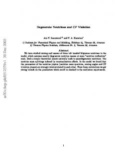
(2.30) Our recipe for determining whether or not a finite non–Abelian group G admits a basis with real Clebsch–Gordan coefficients, using the twisted Frobenius–Schur indicator, is outlined in figure 1.

order |G| of G is odd

G has class–inverting involutory automorphisms

no

yes

G has only irreps of odd dimension

no no

yes

there exists no basis with real CG’s

no

yes there is an automorphism u with all FSu ’s equal to +1

yes

there exists a basis with real CG’s

Figure 1: This flowchart displays a possible sequence of steps one could follow to determine whether a finite non–Abelian group G admits a basis with real Clebsch–Gordan coefficients. The twisted Frobenius–Schur indicator for an irreducible representation r i and an automorphism u is defined as FSu (r i ) :=

1 X 1 X χri(g u(g)) = tr [ρri(g) ρri(u(g))] |G| g∈G |G| g∈G 1 X = [ρri(g)]αβ [ρri(u(g))]βα , |G| g∈G

(2.31)

where we sum over the matrix indices α and β. From the definition it is immediately clear that for u ≡ id one recovers the original Frobenius–Schur indicator. The proof of the statements in equation (2.30) is based on the well–known Schur orthogonality relation for the irreducible representations r i of the group G (see e.g. [17, p. 37]), X g∈G

  [ρri(g)∗ ]αβ ρrj (g) γδ =

|G| δij δαγ δβδ . dim r i

9

(2.32)

The irreducible representations realized by ρri(g) and [ρri(u(g))]∗ are equivalent for all i if and only if u is class–inverting. Hence, if u is not class–inverting, according to equation (2.32), the twisted Frobenius–Schur indicator vanishes for at least one irreducible representation. Let now u be class–inverting. Then there is a unitary matrix Uri for each irreducible representation r i such that ρri(u(g)) = Uri ρri(g)∗ Ur†i ,

∀i.

(2.33)

Inserting this into the twisted Frobenius–Schur indicator and simplifying the expression, one arrives at   1 X [ρri(g)]αβ [Uri ]βγ [ρri(g)∗ ]γδ Ur†i δα FSu (r i ) = |G| g∈G   |G| 1 [Uri ]βγ Ur†i δα δαγ δβδ |G| dim r i
1 1 = tr Uri Ur∗i = tr (Vri ) . dim r i dim r i

(2.32)

=

(2.34)

As shown in section 2.3, Vri is ±1 if and only if u is an involution, where plus signals a symmetric and minus an anti–symmetric matrix Uri . Hence, if and only if u is a class– inverting involution, the twisted Frobenius–Schur indicator is ±1 for all irreps r i . Furthermore, u is a Bickerstaff–Damhus automorphism if and only if equation (2.25) holds with symmetric matrices Uri . Thus, u is a BDA if and only if the twisted Frobenius– Schur indicators of all irreducible representations of G are +1. This completes the proof of equation (2.30). It is important to note that the twisted Frobenius–Schur indicator can vanish for higher–order automorphisms even though they are class–inverting. For such automorphisms, one can define an extended version of the indicator, which again has the property to be ±1 for all irreps in the class–inverting case and 0 for some irrep otherwise. Let n = ord (u)/2 for even–order and n = ord (u) for odd–order automorphisms. Then the nth extended4 twisted Frobenius–Schur indicator FS(n) u (r i ) :=

(dim r i )n−1 |G|n

X g1 ,...,gn ∈G


χri g1 u(g1 ) · · · gn u(gn )

(2.35)

is ±1 for all irreducible representations if u is class–inverting and 0 for at least one irrep if not. A proof of this statement is given in appendix C.3.

2.6

Three types of groups

The twisted Frobenius–Schur indicator can be used to categorize finite groups into three classes. In order to do so, one has to compute the indicator for all involutory automor4

The 1st extended twisted Frobenius–Schur indicator FS(1) u is identical to the regular twisted FSu .

10

phisms uα of the specific finite group G.5 A code for the group theory software GAP [15] that performs this task is shown in appendix B. There are then three cases: Case I: for all involutory automorphisms uα of G there exists at least one representation r i for which FSuα (r i ) = 0. In this case, the discrete symmetry G does not allow us to define a proper CP transformation in a generic setting. Case II: for (at least) one involutory automorphism u of G, the FSu ’s for all representations are non–zero. Then there are two sub–cases: Case II A: all FSu ’s are +1 for one of those u’s. Then this u is a BDA and there exists a basis with real Clebsch–Gordan coefficients. u can be used to define a proper CP transformation in any basis.6 Case II B: some of the FSu ’s are −1 for all such u’s. Then there is no BDA, and, hence, one cannot find a basis in which all CG’s are real. Yet any of these u’s can be used to define a proper CP transformation. Depending on which case applies to G, we will from now on refer to G as being of type I, type II A and type II B, respectively (see figure 2). In table 2.1, we list for each of the types several examples. Let us also comment that, when building a concrete model, one may still be able to define a proper CP transformation even in the type I case by not introducing any representation which has a zero FSu . That is, groups of type I generically violate CP, but physical CP violation is not guaranteed in non–generic models. We will explain this statement in more detail in section 3.1.

2.7

Physical CP transformations for type II groups

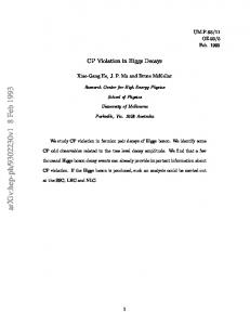
Let us now discuss in more detail the proper physical CP transformations for type II groups and explore under which conditions they can be imposed as a symmetry. Since, as discussed in section 2.3, we have not found any higher–order class–inverting automorphism without a corresponding involutory automorphism that has the same physical implications, we specialize to the case of involutory automorphisms to simplify the discussion. More precisely, one would have to calculate the FS(n) u ’s for all automorphisms. The difference, however, is only relevant for the categorization if all class–inverting automorphisms of G square to a non–trivial outer automorphism. Groups in which this is the case would be classified as type II B. However, an extensive scan (cf. section 2.3) for such groups did not yield any result. On the other hand, we were also not able to prove that such groups cannot exist. 6 Note that these groups can have additional class–inverting involutory automorphisms that are not BDAs. 5

11

group G with automorphisms u

there is a u for which no FS(n) u is 0

no yes

Type I: generic settings based on G do not allow for a physical CP transformation

yes

Type II: u defines a physical CP transformation

there is an involutory u for which all FS(1) u are +1 no

Type II A: there is a CP basis in which all CG’s are real

Type II B: there is no basis in which all CG’s are real

Figure 2: This flowchart displays how the regular and extended twisted Frobenius–Schur indicators FSu and FS(n) u allow us to distinguish between the three types of groups. The integer n is n = ord(u)/2 for even and n = ord(u) for odd ord(u). 2.7.1

Existence of CP transformations

It has been shown in [20] that matrices Uri which solve (2.16) and hence allow for generalized CP transformations g CP

r i 7−−→ Uri r i ∗ ,

(2.36)

exist for all irreducible representations r i if and only if the group exhibits a class– inverting automorphism. To simplify the discussion, one can work in special bases that are particularly convenient for the analysis of CP properties.7 The general situation for class–inverting automorphisms is discussed in [21]; however, since we are dealing with class–inverting and involutory automorphisms, we know that the matrices Uri are either symmetric or anti–symmetric, UrTi = ±Uri [20], cf. the discussion around equation (2.22). This leads to even simpler standard forms than in the general case. In fact, any unitary (anti–)symmetric matrix U can be written as U = W ΣWT , 7

(2.37)

These bases can have other deficiencies, see section 3.2.

12

group Z5 o Z4 SG (20,3)

T7 ∆(27) Z9 o Z3 (21,1) (27,3) (27,4)

(a) Examples for type I groups. Generally, all odd order non–Abelian groups are of this type with the caveat of groups that have a class–inverting automorphism that squares to a non–trivial outer one.

group S3 Q8 A4 Z3 o Z8 SG (6,1) (8,4) (12,3) (24,1)

T0 S4 A5 (24,3) (24,12) (60,5)

(b) Examples for type II A groups. The dihedral and all Abelian groups are also of this type.

group Σ(72) ((Z3 × Z3 ) o Z4 ) o Z4 SG (72,41) (144,120) (c) Examples for type II B groups.

Table 2.1: Examples for the three types of groups: (a) I, (b) II A and (c) II B with their common names and SmallGroups library ID of GAP [15]. with unitary W and  Σ+ =         Σ = Σ− =        

1,  −1     

if U is symmetric, 

1 ..

. −1

    , if U is anti–symmetric.  1 

(2.38)

Note that, since representation matrices always have full rank, the anti–symmetric case does not arise for odd–dimensional irreps [20], i.e. Σ always has full rank. We can, hence, perform the unitary basis change r i → Wr†i r i ,

ρri (g) → Wr†i ρri (g) Wri

∀g∈G,

(2.39)

such that in the new basis the matrices Uri take the simple form Uri → Wr†i Uri Wr∗i = Σri .

(2.40)

For type II A groups, all the Σri ’s equal the identity matrix and the new basis is a CP basis. In this basis all Clebsch–Gordan coefficients are real [16].

13

Let us now investigate under which conditions CP can be imposed as a symmetry. In the most general case, we can write the contraction of two multiplets x and y transforming in irreducible representations r(x) = r x and r(y) = r y to a representation r(z) = r z as   (2.41) (x ⊗ y)rz µ = Cµ,αβ xα yβ = xT Cµ y , where α and β denote the vector indices of x and y, and Cµ,αβ are the Clebsch–Gordan coefficients for the µth component of the resulting representation vector. In the last step we have switched to matrix notation, i.e. Cµ is a matrix, and x and y are vectors. We will also need the complex conjugate of the contraction, which reads   ∗ x∗α yβ∗ = x† Cµ∗ y ∗ . (2.42) (x ⊗ y)∗rz µ = Cµ,αβ In what follows, we will refer to (x ⊗ y)rz as a “meson” and to x and y as its “constituents”. The generalized CP transformation acts on x and y as specified in equation (2.36) with the matrices (Urx )αβ and (Ury )αβ , respectively. From this, we can derive the CP transformation of the meson (x ⊗ y)rz ,   g CP (x ⊗ y)rz µ = xT Cµ y 7−−−→ x† UrTx Cµ Ury y ∗ . (2.36)

(2.43)

In general, also a multiplet z in the representation r z will transform under the generalized CP transformation with some matrix Urz , such that one might demand that   CP   g (x ⊗ y)rz µ − 7 −→ (Urz )µν (x ⊗ y)∗rz ν

(2.42)

=

  (Urz )µν x† Cν ∗ y ∗ .

(2.44)

Comparing (2.44) with (2.43), we obtain the condition !

UrTx Cµ Ury = (Urz )µν Cν ∗ ,

(2.45)

for the consistency of meson and constituent transformations. Recall that the matrices Urx , Ury , and Urz are representations of a class–inverting automorphism and hence are given by the solutions of (2.16). However, the fact that the matrices fulfill (2.16) does not imply that they also solve (2.45). In other words Urx , Ury , and Urz , in general, do not satisfy (2.45). The existence of an automorphism for which the matrices which solve (2.16) also satisfy (2.45) is a non–trivial property of a group.8 At this point, let us note that we are free to re–define phases in the definition of • the Clebsch–Gordan coefficients Cµ,αβ , i.e. one global phase for each r z appearing in the contraction of r x and r y ; • the CP transformations Urx , Ury and Urz . 8

The Clebsch–Gordan coefficients determine a group up to isomorphism [22].

14

This freedom of global phase choices can obscure possible solutions to (2.45) (cf. the discussion around (3.16)). Whether or not one can solve (2.45) is most conveniently analyzed in the basis (2.39), in which (2.45) reads !

∗

ΣTrx Cµ0 Σry = (Σrz )µν (Cν0 ) .

(2.46)

Here we have introduced the basis–transformed Clebsch–Gordan coefficients Cµ0 := WrTx Cµ Wry .

(2.47)

Whether or not (2.45) (or equivalently (2.46)) can be solved depends on the specific automorphism we use to define CP and, hence, on whether the group is type II A or type II B. In the case of type II A groups, the underlying automorphism of the CP transformation is a BDA and, hence, all Σri ’s equal the identity (because all matrices Uri are unitary and symmetric). Therefore, all the Clebsch–Gordan coefficients are real [16] such that equation (2.46) is trivially fulfilled. This statement is trivial in the CP basis but, of course, holds for all other bases as well. Hence the Uri indeed provide us with a solution to equation (2.45). In other words, for type II A groups one can always g follows from the find matrices Uri such that the transformation of a meson under CP (generalized) CP transformation properties of its constituents. We remark that, as we shall demonstrate in an example in section 3.2, the CP basis often turns out not to be the most convenient choice for analyzing a model. If instead the class–inverting and involutory automorphism used to define CP is not a BDA, as is always the case for type II B groups, some of the Uri ’s are anti–symmetric and the existence of a solution to (2.46) is not guaranteed. One can, however, use the symmetry properties of Σrx , Σry and Σrz to check whether a solution is possible. If both Σrx and Σry are either symmetric or anti–symmetric, Σrz has to be symmetric, while in the mixed case Σrz has to be anti–symmetric. In all other cases, (2.46) has no solution. In order to see this, consider, for example, the case of two representations r x and r y transforming with two symmetric matrices Σrx and Σry , and contracting to a representation r z transforming with an anti–symmetric Σrz . Then we see that (2.46) implies that C10 = (C20 )∗

and C20 = − (C10 )∗ ,

(2.48)

such that Clebsch–Gordan coefficients Cµ0 have to vanish, which is obviously a contradiction. This means that a solution to (2.46) is not possible. Hence, if a group allows for such mixed contractions then it is not possible to make all mesons transform in consistency with their constituents. This has striking consequences for the CP properties of a model because, as we will also show in an explicit example in section 3.3, physical CP conservation then implies the absence of the problematic terms from the Lagrangean. 2.7.2

CP transformations and constraints on couplings

Let us now discuss how the CP transformation (2.36) constrains the physical coupling coefficients of a model. Consider a model with some fields furnishing the representa-

15

tions r x and r y . The presence of a contraction (2.41) (with coupling coefficient c) in the Lagrangean implies also the presence of the conjugate contraction (2.42) (with the complex conjugate coupling) in order to guarantee the reality of the Lagrangean. The couplings are, up to the global factor c, given by the Clebsch–Gordan coefficients Cµ . If a theory is invariant under the symmetry, all contractions have to be trivial singlets and therefore the only relevant case is when (Urz )µν is trivial and µ only takes on the value 1. The condition for the term c xT Cµ y to conserve CP then is given by !

∗ c UrTx Cµ=1 Ury = c∗ Cµ=1 ,

(2.49)

which is a simplified version of the consistency condition (2.45). If the corresponding conditions are fulfilled for all contractions present in the Lagrangean, CP is conserved. Note that adding a phase to the generalized CP transformations Urx or Ury is nothing but a simple rephasing of fields. We conclude that, for type II A groups, CP is automatically conserved if there is enough rephasing freedom of fields to render all couplings real, i.e. the corresponding phases unphysical, simply because equations (2.49) are already fulfilled from the group structure. A sufficient number of field redefinitions, however, may not be possible in generic models (see e.g. [23] for criteria), in which case CP can be explicitly violated by the physical phases of couplings. Turning this around, we see that imposing the generalized CP transformation as a symmetry for type II A groups forces all couplings to be real (up to the above–mentioned freedom coming from field redefinitions). The situation for type II A groups, therefore, is somewhat similar to the familiar case where only continuous symmetries such as SU(N ) are present. On the other hand, in the case of type II B groups, some representations may contract in such a way as to make it impossible to solve the appropriate analogue of (2.49). Thus, the corresponding terms cannot be part of the Lagrangean if CP is to be conserved. It is clear from the discussion in section 2.3 that imposing CP in this case implies the presence of an additional Z2 symmetry related to V . It is this Z2 which prohibits exactly the problematic contractions. That is, type II B groups can have the unusual property that CP invariance forbids certain couplings rather than just restricting the phases of the coefficients. Let us remark that, in principle, it is conceivable that the structure of a type II B group is such that it does not allow for CP violating contractions. This is the case if and only if the Z2 symmetry related to the element represented by V is already part of the group. For all examples we have found and given in table 1(c) this is not the case, and the groups have to be extended (trivially) by the Z2 in order to warrant CP conservation. Although we cannot make a general statement on when a group is extended, we can prove it for the special case of ambivalent type II B groups and inner automorphisms.9 Consider first the identity automorphism u(g) = g. For this automorphism, the twisted Frobenius–Schur indicator coincides with the original, un– twisted indicator, i.e. FSu=id (r i ) = ±1 for real and pseudo–real irreps r i , respectively. 9

A group is called ambivalent if it possesses only real and pseudo–real irreducible representations. For such groups, inner automorphisms are class–inverting.

16

Hence, Vri = 1 for real and Vri = −1 for pseudo–real representations. However, it has been shown in [20] that an ambivalent group with an element whose representation matrices are given by these particular Vri has a basis with real CG coefficients. Thus, G would be of type II A, which contradicts the assumption that the group is type II B. Hence, there can be no such group element. The argument can be extended to all inner automorphisms noting that the Vri belonging to these automorphisms are connected to the Vri of the identity by multiplication with a group element (cf. appendix C.1 and footnote 18). In summary, imposing a CP transformation which is defined via in inner automorphism of an ambivalent type II B group always extends the finite symmetry (trivially) by a Z2 factor. We conclude that for groups of type II it is always possible to define a physical CP transformation in a model–independent way. Whether or not it is broken then depends on the details of the model. Below, in sections 3.2 and 3.3 we will present examples illustrating the CP properties of such groups.

3

Examples

3.1

Example for a type I group: ∆(27)

In what follows, we substantiate the statement that type I groups generically violate CP, focusing on a toy model based on the group ∆(27). 3.1.1

Decay amplitudes in a toy example based on ∆(27)

Let us consider a toy model based on the symmetry group ∆(27). The necessary details on the group are summarized in appendix A.2. We introduce three complex scalars S, X and Y transforming as 10 , 11 and 13 as well as two sets of fermions Ψ and Σ, transforming as 3 each. Furthermore, we assume that there is a U(1) symmetry under which Y is neutral, Ψ has charge qΨ , Σ has charge qΣ , and S and X both have charge qX = qΨ − qΣ 6= 0. Then the renormalizable interaction Lagrangean reads10 h h
i
i + g X11 ⊗ Ψ ⊗ Σ 12 Ltoy = f S10 ⊗ Ψ ⊗ Σ 10 10 10 h h
i
i + hΨ Y13 ⊗ Ψ ⊗ Ψ 16 + hΣ Y13 ⊗ Σ ⊗ Σ 16 + h.c. 10

ij

ij

= F S Ψi Σj + G X Ψi Σj + The “Yukawa” matrices are given by   0 1 0 F = f 13 , G = g  0 0 1  1 0 0

10

HΨij

Y Ψi Ψj +

HΣij

Y Σi Σj + h.c. .

 and HΨ/Σ = hΨ/Σ

 1 0 0  0 ω 2 0  , (3.2) 0 0 ω

where f , g, hΨ , and hΣ are complex couplings and we define ω := e2π i/3 . 10

There might also a cubic Y coupling, which is, however, irrelevant for our discussion.

17

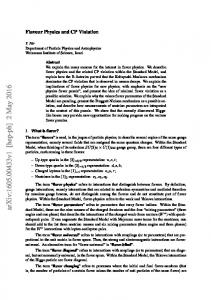
(3.1)

Let us now study the decay Y → ΨΨ. Interference between tree–level and one–loop diagrams (figures 3(a)– 3(c)) leads to a CP asymmetry εY →ΨΨ , which is proportional to h  i h  i εY →ΨΨ ∝ Im [IS ] Im tr F † HΨ F HΣ† + Im [IX ] Im tr G† HΨ G HΣ† = |f |2 Im [IS ] Im [hΨ h∗Σ ] + |g|2 Im [IX ] Im [ω hΨ h∗Σ ] .

(3.3)

Here IS = I(MS , MY ) and IX = I(MX , MY ) denote appropriate phase space factors and the loop integral, which are non–trivial functions of the masses of S and Y , and X and Y , respectively. Note that εY →ΨΨ is (i) invariant under rephasing of the fields, (ii) independent of the phases of f and g, and (iii) independent of the chosen basis as it is proportional to the trace of coupling matrices. Notice, however, that the asymmetry can vanish if there is a cancellation between the two terms, which would require a delicate adjustment of the relative phase ϕ := arg(hΨ h∗Σ ) of hΨ and hΣ . In what follows, we will argue that if such a cancellation occurs, this is either (i) a consequence of a larger discrete symmetry than ∆(27) being present or (ii) it is not immune to quantum corrections. In the first case, a new symmetry has to be present which relates S and X in such a way as to guarantee MS = MX and |g| = |f |, as well as hΨ and hΣ to warrant ϕ = −2π/6. Clearly, this cannot be due to an outer automorphism and, hence, no CP transformation of a ∆(27) setup since such transformations never relate the trivial singlet 10 to other representations. If such a symmetry exists, it has to enhance the original flavor symmetry of the setup, and it is, therefore, no longer appropriate to speak of a ∆(27) model. In the second case, given that Im [IS ] 6= Im [IX ] for MS 6= MX , an adjustment which cancels the asymmetry will require arg(hΨ h∗Σ ) to be different from −2π/6 in general. Note that the diagrams of figures 3(b) and 3(c) also yield vertex corrections which are relevant for the renormalization group equations (RGEs) for hΨ and hΣ . These equations are given by11
dhΨ = hΨ a |hΨ |2 + b |hΣ |2 + . . . + c hΣ dt
dh Σ = hΣ a |hΣ |2 + b |hΨ |2 + . . . + c hΨ 16π 2 dt

16π 2

 2  |f | + ω 2 |g|2 ,

(3.4a)

 2  |f | + ω |g|2 ,

(3.4b)

where t = ln(µ/µ0 ) is the logarithm of the renormalization scale, a, b and c are real coefficients, and the omission represents terms like the square of the gauge coupling. This leads to an RGE for hΨ h∗Σ with the structure 16π 2 11


  d (hΨ h∗Σ ) = hΨ h∗Σ × real + c |hΨ |2 + |hΣ |2 |f |2 + ω 2 |g|2 . dt

Note that G HΨ/Σ G† = ω 2 HΨ/Σ .

18

(3.5)

F Ψ

Y

Ψ

Σ

Y

HΨ

HΣ

S

Σ

(a)

(b) G′

G

Ψ

Ψ Σ

Σ

Y

Ψ

F†

Ψ

HΣ

Y

X

HΣ

Z

Σ

Σ G†

Ψ

G′

(c)

†

Ψ

(d)

Figure 3: Diagrams relevant for CP violation in Y → ΨΨ at tree level and 1–loop. The only value of the relative phase ϕ that is stable under the RGE is, thus, given by ϕ = ϕ∗ = arg (|f |2 + ω 2 |g|2 ). Therefore, we see that, if one imposes that (3.3) vanishes at one renormalization scale, this relation will be violated at other scales provided that Im[IS ] 6= Im[IX ]. Hence, even if one adjusts the phases of hΨ and hΣ by hand, this relation will be destroyed by quantum corrections. We note that such considerations can always be used in order to see if a particular relation is a consequence of a symmetry, in which case it has to respect quantum corrections, or not. Altogether, we conclude that this simple setting based on ∆(27) generically violates CP. The reason behind this is that any conceivable generalized CP transformation is inconsistent with ∆(27) — simply due to the fact that the group (with the field content chosen) does not allow for a class–inverting automorphism. Hence any transformation which relates each field to its complex conjugate, if simply imposed on the theory, would map ∆(27)–invariants to non–invariants, similarly to what happened around equation (2.12), but without the possibility of “repairing” the transformation. Let us point out that due to the peculiarities of the example model, there is neither a

19

U(1) charge asymmetry nor a left–right asymmetry produced by the CP violating decay. In general, however, there seems to be no obstacle in constructing such models. Note also that it is, in principle, possible to distinguish Y from Y ∗ by measuring the relative branching fraction of the decays to ΨΨ and ΣΣ, where a pure sample of, say, Y particles could be generated if we couple it to a pair of chiral fermions. 3.1.2

Spontaneous CP violation with calculable CP phases

Let us next discuss how one could possibly restore CP invariance by enlarging the symmetry group, and how this can lead to the possibility of breaking CP spontaneously with calculable CP phases. Imposing a symmetry that ensures the vanishing of the decay asymmetries is possible if the field content of a theory allows us to combine fields which transform as irreducible representations of ∆(27) to multiplets of a larger group, which then itself has an appropriate class–inverting involutory automorphism, i.e. a proper CP transformation. In order to see how this could work, let us replace S by a field Z, transforming in the non–trivial one–dimensional representation 18 and still carrying the same U(1) charge as X. This will lead to an allowed coupling h
i Z (3.6) + h.c. = (G0 )ij Z Ψi Σj + h.c. Ltoy = g 0 Z18 ⊗ Ψ ⊗ Σ 14 10

with the “Yukawa” matrix   0 0 ω2 G0 = g 0  1 0 0  . 0 ω 0

(3.7)

Instead of the process shown in figure 3(b), one now has to take into account the one– loop diagram for the Y decay displayed in figure 3(d), which contributes to the decay asymmetry as εZY →ΨΨ ∝ |g 0 |2 Im [IZ ] Im[ω 2 hΨ h∗Σ ] .

(3.8)

The statement that CP is generically violated still holds. However, the total CP asymmetry of the Y decay vanishes if (i) MZ = MX , (ii) |g| = |g 0 |, and (iii) ϕ = 0. It is possible to understand this CP conserving spot in parameter space from the fact that one can enhance the flavor symmetry beyond ∆(27). Here this can happen via the (outer) automorphism u3 of ∆(27) (details are given in appendix A.2) which transforms u

3 X ←−→ Z,

u

Y −−3→ Y ,

u

Ψ −−3→ Uu3 ΣC

u

and Σ −−3→ Uu3 ΨC ,

(3.9)

with Uu3 given in equation (A.16). This symmetry is consistent with the U(1) symmetry (for the choice qΣ = −qΨ ) and naturally ensures relations (i)–(iii), thereby granting the absence of CP violation. Let us stress that this is not a CP symmetry of the ∆(27) model, but instead enhances the flavor symmetry of the setup from ∆(27) to SG(54, 5) — and this bigger group itself then has an appropriate class–inverting involutory automorphism

20

which ensures CP conservation. The bigger symmetry can be constructed as the semi– direct product of ∆(27) and the symmetry u3 [12, 13]. Under this bigger symmetry, the previously distinct fields X and Z get combined to a doublet, Ψ and ΣC get combined to a hexaplet and Y stays in a non–trivial one–dimensional representation. Then, since we have enough fields at hand to render all coupling phases unphysical, the class–inverting involutory automorphism of SG(54, 5), which is a physical CP transformation, is an accidental symmetry of the setting. Note that if the relations (i)–(iii) are fulfilled, the quantum corrections to the relative phases of hΨ and hΣ vanish. This substantiates the statement that one can use the behavior under the renormalization group to check whether or not certain relations are caused by a symmetry. Interestingly, it is possible to spontaneously break the larger group SG(54, 5) down to ∆(27) by the VEV of a (U(1) neutral) field φ in the real non–trivial one–dimensional representation of SG(54, 5). The field φ couples to the scalars, thus giving rise to a mass splitting,  

µ φ 2 2 2 2 2 (3.10) Ltoy ⊃ M |X| + |Z| + √ hφi |X| − |Z| + h.c. , 2 with µ denoting a mass parameter. However, φ does not couple to, i.e. alter, the Yukawa couplings of X, Y , and Z at the renormalizable level. Note that, given an appropriate coupling, the φ VEV will also split the masses of the fermions, thus making them distinguishable. Therefore, after the breaking, relations (ii) and (iii), i.e. the equalities |g| = |g 0 | and hΨ = hΣ , still hold, while due to the mass splitting the relation (i) gets destroyed, i.e. MX 6= MZ . As a consequence, CP is violated spontaneously and all the phases which appear in the CP asymmetry εY →ΨΨ ∝ |g|2 |hΨ |2 Im [ω] (Im [IX ] − Im [IZ ]) ,

(3.11)

are independent of the couplings, i.e. calculable. We have, hence, obtained a simple recipe for constructing models of spontaneous CP breaking. One starts with a type II group GII which contains (and can be spontaneously broken down to) a type I group GI . At the level of GII , one imposes the generalized CP transformation, such that at this level CP is conserved. After the spontaneous breaking GII → GI CP will, at least generically, be broken. In the example discussed above, the CP phases are even calculable. A more detailed discussion of these issues will be presented in a subsequent publication. 3.1.3

CP–like symmetries

Let us also emphasize that not every outer automorphism which is imposed as a symmetry does lead to physical CP conservation. Consider for example the outer automorphism u5 given in (A.15e), which is the same as u in [12].12 The only way in which u5 can 12

In HLS [12] the automorphism is defined as u : (A, B) → (A B 2 A B, A B 2 A2 ) while in (A.15e) u5 : (A, B) → (B A2 B 2 , A B 2 A2 ). However, as A B 2 A = B A2 B, these operations coincide.

21

act consistently with all symmetries (again for the choice qΣ = −qΨ ) is to exchange the fermions, u

X −−5→ X ∗ ,

u

Z −−5→ Z ∗ ,

u

Y −−5→ Y ∗ ,

u

Ψ −−5→ Uu5 Σ ,

u

and Σ −−5→ Uu5 Ψ . (3.12)

Clearly, this transformation maps fields with opposite U(1) charges onto each other, i.e. acts like a charge conjugation on the U(1). Hence this is not an enhancement of the flavor symmetry. It is, however, not a physical CP symmetry either since not all representations of ∆(27) are mapped to their complex conjugate representations, in particular 3 → 3. That is, if one were to entertain the possibility that, in a more sophisticated model, the 3–plet describes some fields that are connected to the standard model, this transformation would not entail a physical CP transformation (see also our earlier discussion in section 2.3). Note that imposing (3.12) will enforce equality between the decay amplitudes of Y → ΨΨ and Y ∗ → ΣΣ but none of the relations (i)–(iii) is fulfilled and thus the physical CP asymmetry of the Y decay, εY →ΨΨ , is still non–vanishing, i.e. physical CP is still violated. For these reasons we prefer to call such a symmetry a “CP–like symmetry” (see section 2.3). In particular, we disagree with the statement made by HLS [12] that an arbitrary outer automorphism can serve as a physical CP transformation. To conclude the discussion of the example, we emphasize that the CP violation in ∆(27) exists solely due to the properties of the symmetry group and is independent of any arguments based on spontaneously breaking this or other symmetries. Yet, as we have seen, it is possible to have settings in which a bigger, CP conserving type II symmetry gets spontaneously broken down to ∆(27). In this case, we have found that the physical CP violating phases are predicted by group theory. 3.1.4

CP conservation in models based on ∆(27)

The alert reader may now wonder how it is possible that CP gets broken spontaneously in ∆(27)–based models [24], i.e. how can it be that there is CP conservation to start with. This is because in the model discussed in [24] only triplet representations are introduced, and there exist involutory automorphisms of ∆(27) for which the FSu ’s for the triplets equal 1 (see table A.3 in appendix A.2, and [14] for examples). This allows one to impose a consistent CP transformation for this non–generic setting. However, once one amends the setting by more than two non–trivial one–dimensional representations, this will no longer be possible. In summary, we see that models based on ∆(27) generically violate CP. This can be avoided by 1. increasing the (flavor) symmetry beyond ∆(27); 2. considering settings in which only a special subset of representations is introduced.

22

R 10 FSu (R) 1

11 1

12 1

20 1

21 1

22 1

3 1

Table 3.1: Twisted Frobenius–Schur indicators for the automorphism (3.13) of T0 . 3.1.5

Comments on the possible origin of a ∆(27) symmetry

It may also be interesting to see how CP violation by discrete flavor symmetries originates from some “microscopic” theory. In [25] it was studied how SU(3) can be broken to ∆(27), yet the discussion is based on certain invariants and it is not clear if or how one can achieve this breaking by giving VEVs to certain representation (cf. the discussion in [26]). However, given that ∆(27) does not allow for a proper CP transformation while SU(3) does, it is tempting to speculate that such a breaking, if possible, will also break CP spontaneously. In [27] it was shown how non–Abelian discrete flavor symmetries arise in certain orbifold compactifications but no type I groups were found. A ∆(27) symmetry can arise from space–group rules in non–Abelian heterotic orbifolds [28,29]13 but it is not yet clear what the (massless) matter content of such settings is, i.e. if there are representations with vanishing FSu for all involutory automorphisms. Similar comments apply to [30], where, in a local construction, also a ∆(27) symmetry was found.

3.2

Example for a type II A group: T0

The group T0 , which is the double covering group of A4 , is an example for a group that admits a basis with real Clebsch–Gordan coefficients. Information on the group structure of T0 and the tensor product contractions in different bases can be found in appendix A.1. T0 has a unique outer automorphism, which swaps each representation with its complex conjugate representation, i.e. which is class–inverting. One particular, involutory representative14 of this outer automorphism is given by u : (S, T ) → (S 3 , T 2 )

y 1i → U1i 1i ∗ ,

2i → U2i 2i ∗ ,

3 → U3 3∗ . (3.13)

One can confirm that this automorphism is indeed a Bickerstaff–Damhus automorphism from the twisted Frobenius–Schur indicators in table 3.1. As in our ∆(27) example, one could also construct an explicit example model based on this group and calculate CP asymmetries. However, as has been pointed out in section 2.7 already, there will be no CP violation originating from the intrinsic properties of T0 , i.e. from the Clebsch–Gordan coefficients. That is, unlike in the ∆(27) case, there g transformation (3.13) available that ensures physical CP conservation. Of is the CP 13

We thank P. Vaudrevange for pointing this out. By definition, all other possible choices of automorphisms representing the unique outer automorphism of T0 are connected to our choice by inner automorphisms. 14

23

course, CP could be violated explicitly if there were not enough field rephasing degrees of freedom to absorb all complex coupling parameter phases. This is, however, not related to the group structure of the model and, thus, is not discussed here. Instead, let us use T0 as an example to discuss realizations of the CP transformation (3.13) in different bases and comment on complications which may arise in some of these bases. For the matrices Uri , with which one has to multiply the representation vectors in addition to the conjugation, HLS [12] obtain15 g CP

1i 7−−→ ω i 1i ∗ , HLS

(0 ≤ i ≤ 2) ,

g CP

2i 7−−→ diag(ψ −5 , ψ 5 ) 2i ∗ , HLS

(3.14a)

(0 ≤ i ≤ 2) ,

g CP

3 7−−→ diag(1, ω, ω 2 ) 3∗

(3.14b) (3.14c)

HLS

with ω = e2πi/3 , as before, and ψ = e2πi/24 . This CP transformation is only unique up to multiplication with T0 elements and can still be amended by phase factors ηCP as in equation (2.4) for each field. However, this only corresponds to the freedom of rephasing fields, and, therefore, one can choose a common phase for all fields in the same T0 representation without loss of generality. Yet, the specific choice made by HLS [12] in combination with the Clebsch–Gordan coefficients of [31, Appendix A] appears inconvenient to us for the following reason. Consider the contraction of ψ in the representation 20 with χ in the 21 to the non– trivial singlet 11 , −1 (ψ ⊗ χ)11 = √ (ψ1 χ2 − ψ2 χ1 ) . 2

(3.15)

It is obvious that this contraction does not acquire a phase under the CP transformation (3.14b) because (3.14b)

ψ1 χ2 − ψ2 χ1 −−−−→ ψ1∗ χ∗2 − ψ2∗ χ∗1 .

(3.16)

However, according to (3.14a), the non–trivial singlet 11 should acquire a phase factor ω. Hence, a composite state in the T0 representation 11 transforms differently under CP from an elementary 11 which, although not inconsistent, is certainly inconvenient. Moreover, this complication is unnecessary as we have shown in section 2.7 because for type II A groups it is always possible to fix the CP transformation phases and the phases of the Clebsch–Gordan coefficients in such a way that the CP transformation behavior of fields, composite and elementary alike, directly follows from their transformation behavior under the discrete flavor group. In the basis of Feruglio et al. with the Clebsch–Gordan phases chosen as shown in 15

Note that HLS [12] use the T0 basis of Feruglio et al. [31, Appendix A] (see also appendix A.1.4).

24

appendix A.1 this more convenient CP transformation takes the form g CP

(3.17a)

g CP

(3.17b)

g CP

(3.17c)

1i 7−−→ 1i ∗ , 2i 7−−→ diag (1, e5π i/6 ) 2i ∗ , 3 7−−→ diag (1, ω, ω 2 ) 3∗ .

Furthermore, it turns out that the chosen basis itself has a certain deficit. The 3 of T0 is a real representation. However, the corresponding representation matrices in the Feruglio et al. basis are complex matrices which means that one cannot consistently describe a field φ in the three–dimensional representation by a triplet of manifestly real scalar fields. One may “rectify” this by imposing a Majorana–like condition which constrains the complex entries of the field to the correct number of degrees of freedom, i.e.   1 0 0 φ∗ = U φ = 0 0 1 φ . (3.18) 0 1 0 This is also reflected by the kinetic term, which is given by 1 1 (∂µ φ ⊗ ∂ µ φ)10 = ∂µ φT U T ∂ µ φ 2 2

(3.19)

and is non–positive definite for real field values. If one instead imposes the Majorana–like condition on the kinetic term, 1 (3.18) 1 ∂µ φT U T ∂ µ φ = ∂µ φ† ∂ µ φ , 2 2

(3.20)

one can see that for the now complex field values the kinetic term is indeed positive definite. Nonetheless, treating φ as a complex field and enforcing a condition like equation (3.18) complicates perturbative computations, and, for performing those, it appears more convenient to avoid such a situation altogether by going to a basis where the triplet representation matrices are all real.16 Such a basis is the “Ma–Rajasekaran basis” [32] (see also appendix A.1.3). In this basis, the CP transformation is given by g CP

(3.21a)

g CP

(3.21b)

1i 7−−→ 1i ∗ , 2i 7−−→ 2i ∗ ,   1 0 0 g CP 3 7−−→ 0 0 1 3∗ . 0 1 0

(3.21c)

16

If only complex fields are present in a model, like in supersymmetric models, this issue does not arise.

25

R 10 FSid (R) 1

11 1

12 1

13 1

2 8 −1 1

Table 3.2: Twisted Frobenius–Schur indicators for the identity automorphisms of Σ(72). Since T0 is of type II A, the group also admits a basis with completely real Clebsch– Gordan coefficients, which is given by the one of Ishimori et al. [33] (see also appendix A.1.4) for the choice p = i and p1 = p2 = 1. In this basis, the generalized CP transformation is identical to conjugation since the matrices Uri are all unit matrices. However, the Ishimori basis again suffers from the issues with real triplet fields. Whether one choice of basis or the other is more convenient depends on the specific model at hand.

3.3

Example for a type II B group: Σ(72)

The non–Abelian group Σ(72) is an example for groups of type II B. Information on the generators, characters and tensor product contractions of this group can be found in appendix A.3. As one can check explicitly with the twisted Frobenius–Schur indicator, Σ(72) has no Bickerstaff–Damhus automorphism, and, therefore, there is no basis of the group in which all Clebsch–Gordan coefficients are real. However, the group is ambivalent, i.e. each conjugacy class contains with an element g also its inverse element g −1 , which makes any class–preserving automorphism at the same time class–inverting. Thus, the identity map, which is trivially an involution, can be used to define a consistent and model–independent CP transformation. The corresponding twisted Frobenius–Schur indicators are shown in table 3.2, where the −1 for the two–dimensional representation signals that this representation transforms with an anti–symmetric matrix under the automorphism, which implies that the transformation is not a BDA. In the basis specified in appendix A.3, the corresponding CP transformation takes a very simple form. In fact, the identity automorphism leads to a CP transformation that acts as id

(M, N, P ) 7−−→ (M, N, P )

y

g CP

1i 7−−→ 1i ∗ ,

g CP

2 7−−→ U2 2∗ ,

g CP

8 7−−→ 8∗ (3.22)

on the irreducible representations, where one should bear in mind that all representations of ambivalent groups are (pseudo–)real. Hence, the CP transformation acts as conjugation on all representations except the 2, which has to be conjugated and multiplied with the anti–symmetric matrix   0 1 U2 = . (3.23) −1 0 Therefore, as described in sections 2.3 and 2.7, imposing this CP transformation as a symmetry enlarges the flavor group by an additional Z2 factor to Σ(72) × Z2 . The additional symmetry generator acts trivially on all representations except for the 2, on

26

which it acts as V2 = U2 U2∗ = −1. Hence, this additional Z2 forbids all terms which contain an odd number of fields in the two–dimensional representation 2. These are terms like L ⊃ c (2 ⊗ (8 ⊗ 8)2 )10

(3.24)

which are exactly the ones that cannot be made CP invariant by any choice of coupling c or by the addition of any other term. On the other hand, if all terms which are prohibited by the Z2 are absent, the discussion of CP violation works in complete analogy to type II A groups.

4

Conclusions

In this study, we have discussed CP transformations in settings with a discrete (flavor) symmetry G. We have shown that physical CP transformations are given by the class–inverting automorphisms of G, which implies that canonical CP transformations necessarily have to be generalized due to the nature of discrete groups. This can only be avoided for certain groups (type II A) in very specific bases, or in models with a non–generic field content. One of the central results of our discussion is that there are discrete groups that automatically violate CP in the sense that they do not allow us to impose a consistent (generalized) CP transformation for a generic field content. More specifically, we have shown that there are three types of discrete groups: Type I: Groups that, in general, violate CP. Such groups do not possess a class– inverting automorphism which would be necessary in order to define a (generalized) CP transformation that can warrant physical CP conservation. In generic settings based on such groups CP is violated explicitly. This statement does not apply to non–generic models. For instance, if a model contains only a subset of irreducible representations for which an automorphism u exists that exchanges each of these representations by its conjugate, one can impose the generalized CP transformation corresponding to u to be a symmetry, and thus guarantee CP conservation. Type II A: Groups that do admit real Clebsch–Gordan coefficients. For such groups one can always define a physical CP transformation and find a CP basis.17 Whether or not CP is violated in settings with type II A symmetries depends on the number of complex couplings versus the number of free field redefinition phases, and, hence, the situation is very similar to that of continuous symmetry groups such as SU(N ). 17

We have also commented on the fact that, although bases with real Clebsch–Gordan coefficients exist for type II A groups, such bases may not be the most convenient choices for performing computations. Possible issues include that it may not be possible to represent real representations by manifestly real fields. In such a case it might be advantageous to work in basis with complex Clebsch–Gordan coefficients and to use a generalized CP transformation with a non–trivial UCP when imposing CP invariance.

27

Type II B: Groups that do not admit real Clebsch–Gordan coefficients but possess a class–inverting automorphism that can be used to define a generalized CP transformation. Apart from the obvious possibility that, like in the case of a type II A symmetry group, CP can be violated explicitly (or spontaneously), here CP violation can arise from the presence of operators which are prohibited by an additional symmetry, which might be introduced when imposing CP invariance. That is, these groups have the unusual property that CP invariance requires certain couplings to vanish rather than just restricting the phases of the coupling coefficients. However, unlike in the type I case, CP can be imposed regardless of the matter content of a model based on a type II B group. We have discussed how one can use the (extended) twisted Frobenius–Schur indicator as a tool to categorize the automorphisms and, henceforth, the discrete groups. As we have seen in an explicit example, spontaneous breaking of CP with calculable phases can be achieved in settings in which a type II group gets broken spontaneously to a type I group. CP violation can then be attributed to some complex Clebsch–Gordan coefficients. That is, the CP phases are predicted by group theory. Another central outcome of our analysis is that some of the transformations that have been coined “generalized CP transformations” in the recent literature are just outer automorphisms, which have, a priori, nothing to do with CP. As we have demonstrated, imposing such a “generalized CP transformation” does not lead to physical CP conservation, but in many cases it enlarges the original (flavor) symmetry G to a larger group such that the setting can no longer be called a, say, ∆(27) model. That is, although proper generalized CP transformations are outer automorphisms of G, in general, outer automorphisms as such have nothing to do with CP invariance. For instance, ∆(27) has several outer automorphisms but does not allow for a consistent CP transformation in a generic setting. As we have discussed in detail, this is because none of the automorphisms is class–inverting.

Acknowledgments We would like to thank Oleg Lebedev, Christian Staudt and Patrick Vaudrevange for useful discussions. M.R. would like to thank the UC Irvine, where part of this work was done, for hospitality. M.-C.C. would like to thank TU M¨ unchen, where part of the work was done, for hospitality. This work was partially supported by the DFG cluster of excellence “Origin and Structure of the Universe”, the Graduiertenkolleg “Particle Physics at the Energy Frontier of New Phenomena” by Deutsche Forschungsgemeinschaft (DFG) and the TUM Graduate School. The work of M.-C.C. was supported, in part, by the U.S. National Science Foundation (NSF) under Grant No. PHY-0970173. The work of K.T.M. was supported, in part, by the U.S. Department of Energy (DoE) under Grant No. DEFG02-04ER41290. M.-C.C. and M.R. would like to thank the Aspen Center for Physics for hospitality and support. M.-.C.C. thanks the Galileo Galilei Institute for Theoretical Physics for the hospitality. This research was done in the context of the ERC Advanced Grant project “FLAVOUR” (267104).

28

A

Group theory

In this appendix we collect information on the groups used in the main text: T0 , ∆(27) and Σ(72). Some of the details were obtained with the help of GAP [15] and the Mathematica–package Discrete [34].

Group theory of T0

A.1

We start by discussing some basic facts on T0 and compare different conventions used in the literature. A.1.1

T0 generators

T0 is generated by the operations S and T where S 4 = T 3 = (S T )3 = e .

(A.1)

There are seven irreducible representations, 1i , 2i and 3, where 0 ≤ i ≤ 2 and the representations 11 and 21 are conjugate to 12 and 22 , respectively. S T

10 1 1

11 1 ω

12 1 ω2

20 S20 T20

21 S21 T21

22 S22 T22

3 S3 T3

Table A.1: Representations of the T0 generators.

A.1.2

T0 tensor products

The T0 tensor product rules are 2i ⊗ 2j = 3 ⊕ 1i+j mod 3 , 2i ⊗ 3 = 20 ⊕ 21 ⊕ 22 , 3 ⊗ 3 = 3s ⊕ 3a ⊕ 10 ⊕ 11 ⊕ 12 . A.1.3

(A.2a) (A.2b) (A.2c)

Ma–Rajasekaran basis for T0

A basis in which the representation matrices for the real triplet representation are manifestly real has been given by Ma and Rajasekaran [32] in the case of A4 . For T0 it is given by √   1 i 2i M √ S2i = − √ , (i = 0, 1, 2) , (A.3a) 2 i −i 3  2      1 0 ω 0 ω 0 M M M , T22 = , (A.3b) T20 = , T21 = 0 ω 0 ω2 0 1

29

S3M

  1 0 0 = 0 −1 0  , 0 0 −1



T3M

 0 1 0 = 0 0 1 . 1 0 0

(A.3c)

The tensor products with the correct phases and correct normalization read (x3 ⊗ y3 )10 = (x3 ⊗ y3 )11 = (x3 ⊗ y3 )12 = (x3 ⊗ y3 )3s = (x3 ⊗ y3 )3a = ψ2i ⊗ χ2j


1i+j

ψ2i ⊗ χ23−i




ψ2i ⊗ χ22−i




ψ2i ⊗ χ21−i




3

3

3

(ψ2i ⊗ x3 )2i (ψ2i ⊗ x3 )2i+1 (ψ2i ⊗ x3 )2i+2

x1 y 1 + x2 y 2 + x3 y 3 √ , 3 x1 y1 + ω 2 x2 y2 + ω x3 y3 √ , 3 x1 y1 + ω x2 y2 + ω 2 x3 y3 √ , 3   x2 y 3 + x3 y 2 1 √ x1 y3 + x3 y1  , 2 x y +x y 1 2 2 1   x2 y 3 − x3 y 2 i √ x3 y1 − x1 y3  , 2 x y −x y 1

2

2

(A.4a) (A.4b) (A.4c) (A.4d)

(A.4e)

1

−1 = √ (ψ1 χ2 − ψ2 χ1 ) , (A.4f) 2   −ψ1 χ1 + √12 (ψ1 χ2 + ψ2 χ1 ) + ψ2 χ2 1   = √ −ω ψ1 χ1 + √12 (ψ1 χ2 + ψ2 χ1 ) + ω 2 ψ2 χ2  , (A.4g) 3 −ω 2 ψ χ + √1 (ψ χ + ψ χ ) + ω ψ χ 1 1 1 2 2 1 2 2 2   1 −ψ1 χ1 + √2 (ψ1 χ2 + ψ2 χ1 ) + ψ2 χ2 1   = √ −ψ1 χ1 + ω 2 √12 (ψ1 χ2 + ψ2 χ1 ) + ω ψ2 χ2  , (A.4h) 3 −ψ χ + ω √1 (ψ χ + ψ χ ) + ω 2 ψ χ 1 1 1 2 2 1 2 2 2   −ψ1 χ1 + √12 (ψ1 χ2 + ψ2 χ1 ) + ψ2 χ2 1   = √ −ω 2 ψ1 χ1 + ω √12 (ψ1 χ2 + ψ2 χ1 ) + ψ2 χ2  , (A.4i) 3 −ω ψ χ + ω 2 √1 (ψ χ + ψ χ ) + ψ χ 1 1 1 2 2 1 2 2 2 √   1 ψ1 (x1 + x2 + x3 ) + 2 ψ2 (x1 + ω 2 x2 + ω x3 ) √ = , (A.4j) 2 ψ1 (x1 + ω x2 + ω 2 x3 ) − ψ2 (x1 + x2 + x3 ) 3 √   1 ψ1 (x1 + ω 2 x2 + ω x3 ) + 2 ψ2 (x1 + ω x2 + ω 2 x3 ) √ = , 2 ψ1 (x1 + x2 + x3 ) − ψ2 (x1 + ω 2 x2 + ω x3 ) 3 (A.4k) √   2 1 √ ψ1 (x1 + ω x22 + ω x3 ) + 2 ψ2 (x1 + x2 + x23 ) = . 2 ψ1 (x1 + ω x2 + ω x3 ) − ψ2 (x1 + ω x2 + ω x3 ) 3 (A.4l)

30

A.1.4

Ishimori et al. basis

Another basis for the triplet representation has been discussed in [33], where one uses √   1 i 2p I √ ∗ , (i = 0, 1, 2) , (A.5a) S2i = − √ −i 3 − 2p  2      ω 0 1 0 ω 0 I I I T20 = , T21 = , T22 = , (A.5b) 0 ω 0 ω2 0 1   −1 2 p1 2 p1 p2 −1 2p2  , (A.5c) S3I =  2 p∗1 ∗ ∗ ∗ −1 2 p 1 p2 2 p2   1 0 0 T3I = 0 ω 0  (A.5d) 2 0 0 ω as generators with p = ei ϕ , p1 = ei ϕ1 , and p2 = ei ϕ2 , where ϕ, ϕ1 , and ϕ2 are arbitrary real phases. The free phases of the triplet representation can be removed by a transformation Se3I = P S3I P † with   1 0 0  . 0 P =  0 e i ϕ1 (A.6) i (ϕ1 +ϕ2 ) 0 0 e The transformation which connects the bases (A.3) and (A.5) for the triplet representations is given by e P ) S3I (U e P )† S3M = (U

e P ) T3I (U e P )† , and T3M = (U

(A.7)

with 

 1 1 1 e = √1  1 ω ω 2  . U 3 1 ω2 ω

(A.8)

Note that for the particular choice of p = i and p1 = p2 = 1, the representation matrices of basis (A.5) fulfill the Bickerstaff–Damhus equation (2.27) for the outer automorphism (S, T ) → (S 3 , T 2 ). Hence, in this particular basis, all Clebsch–Gordan coefficients are real. This has also been found in an explicit computation [33]. Another basis commonly used in the literature is the one of Feruglio et al. [31, Appendix A], which can be obtained from (A.5) by setting p1 = p2 = e2πi/3 and p = e2πi/24 . We adjust the global phases of the tensor product contractions in this basis such that for the CP transformation (3.17) compound states transform like elementary states

31

and obtain (x3 ⊗ y3 )10 = (x3 ⊗ y3 )11 = (x3 ⊗ y3 )12 = (x3 ⊗ y3 )3s = (x3 ⊗ y3 )3a = ψ2i ⊗ χ2j


1i+j

ψ2i ⊗ χ23−i




ψ2i ⊗ χ22−i




ψ2i ⊗ χ21−i




=

3

=

3

=

3

=

(ψ2i ⊗ x3 )2i = (ψ2i ⊗ x3 )2i+1 = (ψ2i ⊗ x3 )2i+2 =

A.2

x1 y 1 + x2 y 3 + x3 y 2 √ , 3 ω (x1 y2 + x2 y1 + x3 y3 ) √ , 3 ω 2 (x1 y3 + x2 y2 + x3 y1 ) √ , 3   2x1 y1 − x3 y2 − x2 y3 1 √ −x2 y1 − x1 y2 + 2x3 y3  , 6 −x y + 2x y − x y 3 1 2 2 1 3   x y − x3 y 2 1  2 3 √ x1 y 2 − x2 y 1  , 2 x y −x y 3

e

1

1

(A.9a) (A.9b) (A.9c) (A.9d)

(A.9e)

3

7i π/12

√ (ψ1 χ2 − ψ2 χ1 ) , 2  1−i  (ψ χ + ψ χ ) 1 2 2 1 2  , i ψ1 χ1 i ω2  ψ2 χ2   i ψ1 χ1  , ψ2 χ2 i 1−i (ψ1 χ2 + ψ2 χ1 ) 2  ψ2 χ 2 (ψ1 χ2 + ψ2 χ1 ) , i ω  1−i 2 i ψ1 χ 1   1 ψ1 χ1 + (1 + i) ψ2 χ2 √ , 3 (1 − i) ψ1 χ3 − ψ2 χ1   ω (ψ1 χ2 + (1 + i) ψ2 χ3 ) √ , (1 − i) ψ1 χ1 − ψ2 χ2 3   ω 2 ψ1 χ3 + (1 + i) ψ2 χ1 √ . 3 (1 − i) ψ1 χ2 − ψ2 χ3

(A.9f) (A.9g)

(A.9h)

(A.9i) (A.9j) (A.9k) (A.9l)

Group theory of ∆(27)

∆(27) is generated by the operations A and B, where A3 = B 3 = (A B)3 = e .

(A.10)

The conjugacy classes are given as C1a : {e} , C3a : {A, BAB 2 , B 2 AB} ,

C3b : {A2 , BA2 B 2 , B 2 A2 B} ,

32

C1a 1 ∆(27) e 10 1 11 1 12 1 13 1 14 1 15 1 16 1 17 1 18 1 3 3 3 3

C3a 3 A 1 1 1 ω2 ω2 ω2 ω ω ω 0 0

C3b 3 A2 1 1 1 ω ω ω ω2 ω2 ω2 0 0

C3c 3 B 1 ω2 ω 1 ω2 ω 1 ω2 ω 0 0

C3d 3 B2 1 ω ω2 1 ω ω2 1 ω ω2 0 0

C3e C3f 3 3 ABA BAB 1 1 2 ω ω ω ω2 ω ω2 1 1 ω2 ω ω2 ω ω ω2 1 1 0 0 0 0

C3g 3 AB 1 ω2 ω ω2 ω 1 ω 1 ω2 0 0

C3h 3 A2 B 2 1 ω ω2 ω ω2 1 ω2 1 ω 0 0

C3i C3j 1 1 AB 2 ABA BA2 BAB 1 1 1 1 1 1 1 1 1 1 1 1 1 1 1 1 1 1 3ω 2 3ω 3ω 3ω 2

Table A.2: Character table of ∆(27). We define ω := e2π i/3 . The conjugacy classes (c.c.) are labeled by the order of their elements and a letter. The second line gives the cardinality of the corresponding c.c. and the third line gives a representative of the c.c. in the presentation specified in the text. C3c C3e C3g C3i

: {B, ABA2 , A2 BA} , : {ABA, A2 B, BA2 } , : {AB, BA, A2 BA2 } , : {AB 2 ABA} ,

C3d C3f C3h C3j

: {B 2 , AB 2 A2 , A2 B 2 A} , : {BAB, B 2 A, AB 2 } , : {AB 2 A, A2 B 2 , B 2 A2 } , : {BA2 BAB} .

(A.11)

There are eleven inequivalent irreducible representations 1i , 3, and 3, where 0 ≤ i ≤ 8. The character table is given in A.2. (HLS) We adopt the labeling of [12] with the difference that in our notation 1i = 1i−1 and use the contractions of [35] translated to our conventions. There appears to be a typographical error in the character table of [35] in which the characters of the two conjugacy classes C10 and C11 should be interchanged. The representations (11 , 12 ), (13 , 16 ), (14 , 18 ), and (15 , 17 ) as well as the triplets are the complex conjugate of each other. For the triplet 3 we use the representation matrices     0 1 0 1 0 0 A = 0 0 1 , B = 0 ω 0  (A.12) 1 0 0 0 0 ω2 and for 3 the respective complex conjugate matrices. This results in the multiplication rule x3 ⊗ y 3 =

9 X

1i ,

(A.13)

i=1

33

where 10 = 11 = 13 = 14 = 15 =

(x1 y 1 + x2 y 2 + x3 y 3 ) √ , 3 (x1 y 2 + x2 y 3 + x3 y 1 ) √ , 3 (x1 y 1 + ω x2 y 2 + ω 2 x3 y 3 ) √ , 3 (x1 y 2 + ω x2 y 3 + ω 2 x3 y 1 ) √ , 3 (x2 y 1 + ω x3 y 2 + ω 2 x1 y 3 ) √ , 3

(A.14a) (x2 y 1 + x3 y 2 + x1 y 3 ) √ , 3 (x1 y 1 + ω 2 x2 y 2 + ω x3 y 3 ) √ = 3 (x2 y 1 + ω 2 x3 y 2 + ω x1 y 3 ) √ = 3 (x1 y 2 + ω 2 x2 y 3 + ω x3 y 1 ) √ = 3

12 =

(A.14b)

16

,(A.14c)

18 17

,(A.14d) .(A.14e)

From the discussion in appendix C it is clear that ∆(27) as a non–Abelian group of odd order does not allow for any class–inverting involutory automorphism. Therefore, there is no possibility of having a physical CP symmetry in a generic setup. There are, however, several outer automorphisms which exchange a subset of representations with their complex conjugates. If one is to construct a model with one of those subsets there is the possibility of imposing physical CP conservation. Altogether there are 46 involutory automorphisms. Some examples are given by u1 : (A, B) → (A, B 2 )

y 11 ↔ 12 , 14 ↔ 15 , 17 ↔ 18 , 3 → Uu1 3∗ , (A.15a)

u2 : (A, B) → (ABA, B)

y 11 ↔ 14 , 12 ↔ 18 , 13 ↔ 16 , 3 → Uu2 3∗ , (A.15b)

u3 : (A, B) → (BAB, B 2 )

y 11 ↔ 18 , 12 ↔ 14 , 15 ↔ 17 , 3 → Uu3 3∗ , (A.15c)

u4 : (A, B) → (AB 2 A, B)

y 11 ↔ 17 , 12 ↔ 15 , 13 ↔ 16 , 3 → Uu4 3∗ , (A.15d)

u5 : (A, B) → (BA2 B 2 , AB 2 A2 )

y 1i ↔ 1i ∗ , 3 → Uu5 3 .

(A.15e)

All other representations stay inert under the transformation, and by 3 → Uui 3∗ we mean that fields in the triplet representation have to be multiplied by the corresponding matrix in addition to a possible conjugation. In our basis, these matrices are given by     ω 0 0 1 0 0 Uu1 = 1 , Uu2 =  0 0 1 , Uu3 = 0 ω 2 0  , 0 1 0 0 0 ω2     1 0 0 0 0 ω2 Uu4 = 0 0 ω  , Uu5 =  0 1 0  . (A.16) 0 ω 0 ω 0 0 The corresponding twisted Frobenius–Schur indicators for all representations are given in table A.3. One can convince oneself by computing all FSu ’s that for models with

34

R 10 FSu1 (R) 1 FSu2 (R) 1 FSu3 (R) 1 FSu4 (R) 1 FSu5 (R) 1

11 1 0 0 0 1

12 1 0 0 0 1

13 0 1 0 1 1

14 0 0 0 0 1

15 0 0 1 0 1

16 0 1 0 1 1

17 0 0 1 0 1

18 0 0 0 0 1

3 3 1 1 1 1 1 1 1 1 0 0

Table A.3: Twisted Frobenius–Schur indicators for some outer automorphisms of ∆(27). C1a 1 Σ(72) e 10 1 11 1 12 1 13 1 2 2 8 8

C3a 8 P 1 1 1 1 2 −1

C2a 9 M2 1 1 1 1 −2 0

C4a 18 MN 1 1 −1 −1 0 0

C4b 18 N 1 −1 1 −1 0 0

C4c 18 M 1 −1 −1 1 0 0

Table A.4: Character table of Σ(72). The conjugacy classes (c.c.) are labeled by the order of their elements and a letter. The second line gives the cardinality of the corresponding c.c. and the third line gives a representative of the c.c. in the presentation specified in the text. fields in more than two non–trivial one–dimensional representations and a triplet it is impossible to find an automorphism that leads to a consistent CP transformation. This is a highly interesting feature of this group.

A.3

Group theory of Σ(72)

The non–Abelian group Σ(72) is isomorphic to the semi–direct product group (Z3 × Z3 ) o Q8 , where Q8 is the quaternion group, and is generated by three generators M , N and P , which fulfill the relations
2 M 4 = N 4 = P 3 = M 2 P −1 = e , M 2 = N 2 , M −1 N = N M , P M P N −1 M P −1 N = e , N P M −1 P = M P N . (A.17) Σ(72) has 6 inequivalent irreducible representations: four one–dimensional (10−3 ), one two–dimensional (2), and one eight–dimensional (8). The characters of Σ(72) are shown in table A.4. From the character table one can also read off the matrix realizations of the generators for the one–dimensional representations. The generators for the two– dimensional representation are given by       0 1 −i 0 1 0 M2 = , N2 = , P2 = , −1 0 0 i 0 1 35

and the three matrices  0 0 0 0  1 0  0 −1 M8 =  0 0  0 0  0 0 0 0  −1 −√3   0  1   0 P8 =  2  0   0   0 0

1 0 0 1 0 0 0 0 0 0 0 0 0 0 0 0 √ 3 −1 0 0 0 0 0 0

  0 0 0 0 0 0 0 0 0 0   0 0 0 0 0    0  , N8 = 0 0 0 0  1 0 0 0 0  0 −1 0 0 1   0 0 1 0 0 0 0 0 0 1  0 0 0 0 0 0 0 0 0 0 0 0   2 0 0 0 0 0    0 2 0 0 0 0  √  , 0  0 0 √ −1 − 3 0  0 0 3 −1 0 0  √   0 0 0 0 −1 − 3 √ 0 0 0 0 3 −1 0 0 0 0 0 0 0 0 0 0 0 0 1 0 0 −1

0 0 0 0 1 0 0 0

1 0 0 0 0 0 0 0

0 1 0 0 0 0 0 0

 0 0 0 0  1 0  0 −1  , 0 0  0 0  0 0 0 0

generate the eight–dimensional representation. The (non–trivial) tensor product contractions of Σ(72) are the following:     1 i x1 y1 x1 y 2 (x10 ⊗ y2 )2 = √ , (x11 ⊗ y2 )2 = √ , 2 x1 y2 2 x1 y 1     1 i x1 y 1 x1 y2 , (x13 ⊗ y2 )2 = √ , (x12 ⊗ y2 )2 = √ 2 −x1 y2 2 −x1 y1 1 (x2 ⊗ y2 )10 = √ (x1 y2 − x2 y1 ) , 2 i (x2 ⊗ y2 )12 = √ (x1 y2 + x2 y1 ) , 2

i (x2 ⊗ y2 )11 = √ (x1 y1 − x2 y2 ) , 2 1 (x2 ⊗ y2 )13 = √ (x1 y1 + x2 y2 ) , 2

(x10 ⊗ y8 )8 = (x1 y1 , x1 y2 , x1 y3 , x1 y4 , x1 y5 , x1 y6 , x1 y7 , x1 y8 )T ,

(x11 ⊗ y8 )8 = (x1 y1 , x1 y2 , −x1 y3 , −x1 y4 , −x1 y5 , −x1 y6 , x1 y7 , x1 y8 )T ,

(x12 ⊗ y8 )8 = (x1 y1 , x1 y2 , −x1 y3 , −x1 y4 , x1 y5 , x1 y6 , −x1 y7 , −x1 y8 )T ,

(x13 ⊗ y8 )8 = (x1 y1 , x1 y2 , x1 y3 , x1 y4 , −x1 y5 , −x1 y6 , −x1 y7 , −x1 y8 )T ,

(x2 ⊗ y8 )81 = (i x1 y2 , −i x1 y1 , i x2 y4 , −i x2 y3 , x1 y6 , −x1 y5 , x2 y8 , −x2 y7 )T ,

(x2 ⊗ y8 )82 = (i x2 y2 , −i x2 y1 , −i x1 y4 , i x1 y3 , −x2 y6 , x2 y5 , x1 y8 , −x1 y7 )T , 1 (x8 ⊗ y8 )10 = √ (x1 y1 + x2 y2 + x3 y3 + x4 y4 + x5 y5 + x6 y6 + x7 y7 + x8 y8 ) , 2 2

36

(x8 ⊗ y8 )11 = (x8 ⊗ y8 )12 = (x8 ⊗ y8 )13 = (x8 ⊗ y8 )21 = (x8 ⊗ y8 )22 = (x8 ⊗ y8 )81 = (x8 ⊗ y8 )82 = (x8 ⊗ y8 )83 = (x8 ⊗ y8 )84 = (x8 ⊗ y8 )85 = (x8 ⊗ y8 )86 = (x8 ⊗ y8 )87 =

B

1 √ (x1 y1 + x2 y2 − x3 y3 − x4 y4 − x5 y5 − x6 y6 + x7 y7 + x8 y8 ) , 2 2 1 √ (x1 y1 + x2 y2 − x3 y3 − x4 y4 + x5 y5 + x6 y6 − x7 y7 − x8 y8 ) , 2 2 1 √ (x1 y1 + x2 y2 + x3 y3 + x4 y4 − x5 y5 − x6 y6 − x7 y7 − x8 y8 ) , 2 2   1 i x2 y1 − i x1 y2 − x6 y5 + x5 y6 , 2 i x4 y3 − i x3 y4 − x8 y7 + x7 y8   1 i x4 y3 − i x3 y4 + x8 y7 − x7 y8 , 2 −i x2 y1 + i x1 y2 − x6 y5 + x5 y6 1 √ (x1 y1 − x2 y2 , −x2 y1 − x1 y2 , x3 y3 − x4 y4 , −x4 y3 − x3 y4 , 2 x5 y5 − x6 y6 , −x6 y5 − x5 y6 , x7 y7 − x8 y8 , −x8 y7 − x7 y8 )T , 1 √ (x3 y5 + x4 y6 , x4 y5 − x3 y6 , x1 y7 − x2 y8 , −x2 y7 − x1 y8 , 2 x7 y1 + x8 y2 , −x8 y1 + x7 y2 , x5 y3 − x6 y4 , x6 y3 + x5 y4 )T , 1 √ (x3 y7 − x4 y8 , −x4 y7 − x3 y8 , x1 y5 − x2 y6 , x2 y5 + x1 y6 , 2 x7 y3 + x8 y4 , x8 y3 − x7 y4 , x5 y1 + x6 y2 , −x6 y1 + x5 y2 )T , 1 √ (x5 y7 − x6 y8 , x6 y7 + x5 y8 , x7 y5 + x8 y6 , x8 y5 − x7 y6 , 2 x1 y3 + x2 y4 , −x2 y3 + x1 y4 , x3 y1 − x4 y2 , −x4 y1 − x3 y2 )T , 1 √ (x5 y3 + x6 y4 , −x6 y3 + x5 y4 , x7 y1 − x8 y2 , −x8 y1 − x7 y2 , 2 x1 y7 + x2 y8 , x2 y7 − x1 y8 , x3 y5 − x4 y6 , x4 y5 + x3 y6 )T , 1 √ (x7 y5 − x8 y6 , x8 y5 + x7 y6 , x5 y7 + x6 y8 , −x6 y7 + x5 y8 , 2 x3 y1 + x4 y2 , x4 y1 − x3 y2 , x1 y3 − x2 y4 , −x2 y3 − x1 y4 )T , 1 √ (x7 y3 − x8 y4 , −x8 y3 − x7 y4 , x5 y1 − x6 y2 , x6 y1 + x5 y2 , 2 x3 y7 + x4 y8 , −x4 y7 + x3 y8 , x1 y5 + x2 y6 , x2 y5 − x1 y6 )T .

A GAP code to compute the twisted Frobenius– Schur indicator

The following code for GAP computes the twisted Frobenius–Schur indicators for all irreducible representations of a finite group G and a given automorphism aut of this group.

37

twistedFS:=function(G,aut) local elG,tbl,irr,fsList; elG:=Elements(G); tbl:=CharacterTable(G); irr:=Irr(tbl); fsList:=List(elG,x->x*x^aut); return List(irr,y->Sum(fsList,x->x^y))/Size(G); end; This code can easily be augmented to compute the nth extended twisted Frobenius–Schur indicator (see appendix C.3). However, due to the large number of group operations, the computation can be very time–consuming. In practice, it might, therefore, be advisable to check directly whether a given high–order automorphisms is class–inverting instead of using the FS(n) u . As an example, one can print out the twisted Frobenius–Schur indicators of a certain group for all its involutory automorphisms. In the example below, the group SG(24, 3), i.e. T0 , is chosen. G:=SmallGroup(24,3);; autG:=AutomorphismGroup(G);; elAutG:=Elements(autG);; ordTwoAut:=Filtered(elAutG,x->Order(x)