Cramer-Rao Bounds for Antenna Array Design - IEEE Xplore

336

IEEE TRANSACTIONS ON SIGNAL PROCESSING, VOL. 54, NO. 1, JANUARY 2006

Cramer-Rao Bounds for Antenna Array Design Houcem Gazzah and Sylvie Marcos

Abstract—We study the impact of the geometry of the (planar) antenna array on the accuracy of the estimated direction(s) of arrivals of an emitting source. We develop explicit Cramer-Rao bounds (CRBs) of the azimuth and elevation angles that show a simple structure. In particular, for a fixed elevation angle, the CRBs are cosine functions of the source azimuth, and so, regardless of the array geometry. The amplitude and extremes of these functions depend on the array geometry. Hence, the array configuration can be chosen in order to ensure a desired (an)isotropic behavior. To do so, we propose a pragmatic methodology that also takes into account the array ambiguity problem. The array design problem is simplified by limiting the array search within a family of V-shaped arrays that are advantageously characterized by a single parameter, the angle between the two branches. A performance measure is proposed, then analytically expressed, to assess the array directivity and gain with respect to the more standardly used uniform circular array. Index Terms—Antenna arrays, direction-of-arrival (DOA) estimation.

I. INTRODUCTION

D

IRECTION OF ARRIVAL (DOA) has been an intensively investigated topic in signal processing, as reflected by a huge literature and numerous techniques [1]. A narrow-band source originates, at a sensor located in the far-field, a signal whose phase depends on the relative position of the source with respect to the sensor. The DOAs of a number of sources can be determined by displaying a larger number of sensors. Estimation techniques include maximum likelihood, beam-forming and eigenspace techniques (among which the popular MUSIC algorithm [2]). Despite a rich DOA literature, limited research has been dedicated to study the impact of the array configuration on the DOA estimation. Very often, only the uniform linear array (ULA) and its two-dimensional (2-D) extensions (L-shaped, cross, square, and rectangular arrays [3]–[5]) have been specifically studied because they are easier to analyze and adapted to fast implementations. Few results are available for the general array geometry. Cramer-Rao bound (CRB)-based analysis is preferred since it is algorithm-independent and describes the best achievable estimation performance. General expressions of the CRB are widely reported [6], but only the single source case is analytically tractable [4], [7]. This case is of practical importance Manuscript received January 7, 2005; revised March 14, 2005. This work was supported in part by the RNRT/LUTECE project. The associate editor coordinating the review of this manuscript and approving it for publication was Dr. Sven Nordebo. H. Gazzah is with the Institute for Digital Communications, School of Engineering and Electronics, The University of Edinburgh, Edinburgh, EH9 3JL, U.K. (e-mail: [email protected]). S. Marcos is with Centre National de la Recherche Scientifique, LSS/Supélec, 91192 Gif sur Yvette, France (e-mail: [email protected]). Digital Object Identifier 10.1109/TSP.2005.861091

because, then, the CRB is attainable by the MUSIC algorithm [7]. What is actually reported in the literature ([4], [7], [8] for example) are analytic expressions of the Fisher information matrix (FIM), rather than the CRB itself. In the 3-D case, the latter is obtained from the former by matrix inversion and was never explicitly expressed. This has, so far, prevented from full characterization of the array geometry affect on estimation errors. The off-diagonal elements of the FIM were helpful only to state the condition (on the array geometry) for uncoupled azimuth and elevation estimation. This condition, retrieved here as (9), was reported as necessary in [9] and as necessary and sufficient in [10] and [11]. The same condition was proved to be sufficient [11] and necessary [12] to ensure isotropic performance. This condition is the only identified result about the array geometry impact on DOA estimation. In our paper, we consider the most addressed case of a planar array with a single 3-D source [4], [10], [12], [13]. In addition to the azimuth and elevation CRBs, we consider the mean square angular error (MSAE) [11], [12] alternatively proposed as a unique (scalar-valued) performance measure. We give explicit expressions of the CRBs and the (asymptotic normalized) MSAE (ANMSAE) as a function of the source DOA and the sensors locations. In contrast to the complex FIM-based CRB expressions [8], [11], [12], the obtained CRBs simply consist of three independent gains which are functions of the azimuth, the elevation and the observation SNR. Furthermore, we prove that the azimuth-dependent gain is a simple cosine function and is the only term that depends on the array geometry. Also, azimuth and elevation CRBs are rotated versions one of the other and the ANMSAE is equal (up to an additive constant that depends on the array-geometry) to the elevation CRB. Hence, from the array geometry point-of-view, this three-dimensional (3-D) estimation scenario can be completely characterized by a scalar-valued function of the source azimuth only. The developed CRB is a powerful tool to investigate the performance of antenna arrays with arbitrary geometry. It confirms existing results on uncoupled/isotropic arrays. As argued in [11] and [12], isotropy is a compelling array design criterion. However, this may depend on the targeted applications. For example, in airborne emergency positioning systems, directive (anisotropic) arrays may be preferred to exploit available a priori knowledge about the source location. The developed CRB proves to be efficient in investigating directive arrays. For instance, we show that DOA estimates can be enhanced in an arbitrarily preselected range of the source location. The narrower the range, the higher the enhancement. Array design should also take into account array ambiguity, a problem deliberately ignored in [12]. Only limited results (limited to first-order rank ambiguity [14]) are available in the literature. They imply that sensors should be sufficiently spaced. We

1053-587X/$20.00 © 2006 IEEE

GAZZAH AND MARCOS: CRBs FOR ANTENNA ARRAY DESIGN

337

If the sensors are identical and omnidirectional and under the far-field assumptions, the -dimensional output of the antenna array can be expressed as phased replicas of the emitted signal, as expressed by the following model

.. .

Fig. 1. Planar array and source DOAs.

present a pragmatic approach of antenna array design. Because the search is restricted to a specific family of (V-shaped) antenna arrays, the array performance is function of a single parameter (here, the angle between the two branches of the V shape). We compare the V-shaped array to the uniform circular array (UCA). In particular, we prove that, for a given range of the V angle, the V-shaped array outperforms the UCA for both azimuth and elevation estimates, and in all look directions. This methodology can be extended to other families of antenna arrays (see [15] for an application to Y-shaped arrays). and the real and imagiIn the paper, we denote by nary parts of , respectively; and by the determinant of the matrix . After introducing the data model in Section II, we prove and discuss the simplified expressions of the CRB and ANMSAE in Section III. In Section IV, we address practical aspects including condition for isotropic arrays and simplifications obtained for (the almost always encountered) axis-symmetrical arrays. In Section V, a class of V-shaped arrays are studied and their directive behavior is analyzed. A conclusion is given in Section VI. II. DATA MODEL We consider, as depicted in Fig. 1, a planar antenna array composed of sensors located in the plane. To each and and sensor , we associate the polar coordinates . A single source, emitthe complex number , impinges on the ting a narrow-band (wavelength ) signal array from the direction given by the azimuth angle and the elevation angle . Similarly as in [16], is measured counterclockwise from the axis, and is measured clockwise from the axis.

where the th component of represents the noise sample collected by the -th sensor. The DOA-parameterized is known as the steering vector. The single gain vector source is an important special case. In fact, there, the MUSIC algorithm, in addition to the maximum likelihood (ML) algorithm, asymptotically (as the number of snapshots tends to infinity) attains the CRB [7]. The MUSIC algorithm has a computational complexity significantly lower than that of the ML technique. Also, in the single source case, the CRB shows a simple structure, directly expressed in terms of the (derivatives of the) steering vector of the unique radiating source. collected at time indexes Snapshots are used by the DOA estimation algorithm. We assume Gaussian, zero-mean and mutually independent source and noise signals. Independent and identically distributed source snapshots are assumed. Noise samples collected from different sensors and/or at different time indexes are assumed and to be mutually independent. We denote for every . It is well known that signal and noise powers are uncoupled from the direction parameters [11] and from the array structure [4]. Hence, we consider the of azimuth and elevation angles, to parameter vector which we associate the 2 2 symmetric CRB matrix

Diagonal entries and refer to the azimuth and elevation CRBs. Under the above assumptions, the CRB is indirectly given by the following expression of the th row th column entry of the FIM ([7, eq. (39)])

(1) for , where and are the partial derivatives of the steering vector with respect to the azimuth and and , reelevation parameters, i.e., spectively. Obviously, this is rather an expression of the FIM. Simplifications of the FIM were given ([8, eqs. (4.5a)–(4.5e)], [9, eq. (7)], [10, eq. (6)]) and used to state conditions on array geometry for uncoupled azimuth and elevation estimation. In [4, eq. (2.8)], the CRB was explicitly developed, but only as a function of the (derivatives of the) steering vector, not allowing further exploitation of the impact of the array geometry on performance.

338

IEEE TRANSACTIONS ON SIGNAL PROCESSING, VOL. 54, NO. 1, JANUARY 2006

III. CRAMER-RAO BOUNDS In this section, we show that the inverted FIM can be greatly simplified. We first define

Fig. 2. Illustration of the linear dependence between azimuth and elevation CRBs, ANMSAE and C ( ) [cf. (3), (7), and (8)]. The thick line in the horizontal left axis represents the interval of possible values.

8

which depend only on the array geometry, and

the other. The key function is -periodical and fluctuates around the mean value which depends on the observation SNR. The array size, but via . For high not the array geometry, also affects SNR and/or large arrays can be approxi. We define the following function of the mated by azimuth

(6) which, consequently, is a measure of the average (over all possible azimuth angles) estimation performance. Function also verifies

(2) We prove in Appendix A that the entries of the CRB matrix are given by

so that, for a source located with an elevation and an arbitrary azimuth, the azimuth and elevation CRBs are (linearly) linked as follows:

(3)

(7)

(4)

This implies that, for a fixed elevation angle, when the azimuth angle changes, one error increases while the other decreases. A simpler (than considering both azimuth and elevation CRBs) alternative performance measure is the (scalar-valued) ANMSAE which is associated to the angle between the bearing vector pointing at the source and its estimator. It is given by [17]

(5) Alternatively to using (1) to prove the above, one can also use the already simplified FIM from [8]–[10]. However, one advantage of our proof is the use of the polar (instead of Cartesian) coordinates of the array sensors. This allows for more compact CRB expressions. The simple expression of the (entries of the) CRB matrix contrasts with the complexity of those given in [4, eq. (2.8)], [11, (eq. 26)], or [12, (6)]. In particular, azimuth and elevation CRBs consist of three separate terms or gains. They are func, the source elevation ( and tions of the SNR ) and the azimuth . Only the last term depends on the array geometry via and , which can be interpreted as the moment-of-inertia of the array, introduced in [8]. Adding/removing a sensor at/from the antenna centroid does not affect and since they change only because (the shape of) decreases/increases as the number of sensors is incremented/decremented. Seen as functions of the azimuth, and are just scaled and -translated versions one of

which, given (7), implies that (8) As a consequence

With respect to (7) and (8), linearly dependent CRBs and ANMSAE appear as redundant performance measures. This is . illustrated in Fig. 2. They can be uniquely represented by Notice that the array geometry and the observation SNR affect and (i.e., the scaling of the axes) and Fig. 2 only via the thick line (i.e., the set of possible values).

GAZZAH AND MARCOS: CRBs FOR ANTENNA ARRAY DESIGN

339

Finally, another scalar-valued measure of the estimation error is the confidence region of the DOA parameter estimates [8], [18]. It is proportional to the determinant of the CRB matrix which can be retrieved from (14) in Appendix A. In particular, it shows to be azimuth independent and inversely proportional . to

B. Axis-Symmetric Arrays Axis-symmetry is not a restrictive condition. It is the case of (almost) all antenna arrays encountered in practice. Without loss of generality, we assume -axis symmetry. One can, then, easily and are real valued, so that show that

IV. SPECIAL CASES

(10)

First, notice that if all sensors are translated in the same replaced by where is an arbitrary complex way ( and remain unchanged. This agrees with number), then the far-field hypothesis. The expressions above are, hence, independent of the choice of the origin. If the origin is chosen at , and and simplify the centroid of the array, then and , respectively. to A. Isotropic and Anisotropic Arrays plays a key role in inter-deIt can be seen that parameter pendence between azimuth and elevation CRBs [cf. (5)] and in their dependence on the source azimuth [cf. (2)]. In concordance with [10] and [9], both uncoupled and isotropic estimation are met iff

If

, minimum and maximum values are attained at , respectively. Otherwise, they are attained at and , respectively. Hence, regardless of the positions of the array sensors, as long as these are symmetric with respect to an axis, the antenna performance is a cosine function of the source azimuth and it is maximum/minimum in the direction of the axis of symmetry and the direction perpendicular to it. To further simplify (10), we assume the sensors coordinates to be determined with respect to the array centroid. We define the normalized (with respect to the wavelength) sensor Cartesian coordinates and

(9) As commented in [11], this condition is not restrictive. It merely imposes a kind of symmetry of the array. An isotropic array . verifies is the key element to evaluate For anisotropic arrays, the array performance. Its extremes within can be shown to be attained if is such that i.e., equals modulo . Minimum and maxare met at perpendicular look directions. imum values of This meets conclusions from [8] where it was proved that the most and least desirable DOAs are always perpendicular to each other and correspond to the principal axes of inertia of the array. are given by Minimum and maximum values of

Now, we prove that if

then, we have

(11) so that we have Proof: First, we make the following simplifications for an arbitrary array geometry (not necessarily axis-symmetrical):

As the source azimuth varies, spans the interval between and , as illustrated by the thick lines in Fig. 2. When (9) is fulfilled, this interval simplifies to a single point. can be interpreted as a performance Finally, because is minimum iff (9) measure, and because, for a fixed is fulfilled, we can conclude that array directivity is obtained at the expense of the average performance. In other words, if sensors are placed in order to enhance the DOA estimation in the neighborhood of a given look direction, then the overall performance degrades.

340

IEEE TRANSACTIONS ON SIGNAL PROCESSING, VOL. 54, NO. 1, JANUARY 2006

For nonreal-valued

, we have so that the above reduces to

Now, if the symmetry with respect to the axis is verified, the . On the other last term is zero, and the above is nothing but hand, while simplifies, because of axis symmetry, to . Straightforward manipulations lead to (11). The condition (9) for isotropy/uncoupled estimation is equivalent to have . If we rewrite (11) as

then, with respect to (3) and (4), and given that the above im, it is clear plies that that fixed values of the azimuth and elevation CRBs at a given look direction imply fixed values of and . Hence, imposing an axis symmetry appears as the natural way to design direcand tive arrays. Without loss of generality, we assume the source to be placed on the axis. The azimuth CRB is minwhile the elevation CRB imum and equals is maximum and equals . In other words, the sensors and coordinates can be independently chosen (while maintaining axis symmetry and centroid at the origin) to meet the desired CRBs. Arbitrary high accuracy can be obtained by largely spacing sensors. In practice, this is not an option because this affects ambiguity. In the next section, we propose a pragmatic approach to design (directive) arrays. V. DESIGN OF DIRECTIVE ARRAYS We address the design of directive arrays where sensors placements are chosen in order to enhance the localization performance in (the neighborhood of) a predetermined look direction. To serve this purpose, we use results from Section IV, but also need to address the antenna ambiguity problem. The so-called rank ambiguity occurs when steering vectors corresponding to different look directions are linearly dependent [2]. This problem was formally stated in [14] but only the single source case is analytically tractable [19], [20]. This is illustrated by the fact that, except for second-order ambiguity [20], no conditions were proposed that guarantee higher-order ambiguity free arrays. A sufficient condition for the uniqueness

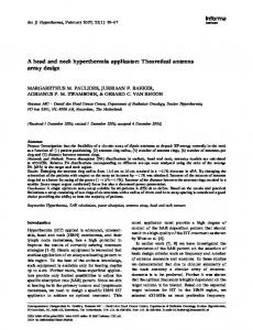
Fig. 3.

V-shaped antenna array.

of the steering vector was given in [14, Th. 9]. It requires minimal spacings between three sensors of the planar array. Generalizations of [14, Th. 9] that involve four sensors are proposed in [19] and [20]. A sufficient and necessary condition was also given in [21]. While interspacing requirements are relaxed, these extensions are impractical because they involve angular parameters. In addition, they assume the source to be in the array plane. We, hence, refer to [14] to solve the first-order ambiguity problem. It is also a simple approach compared to [22] where ambiguity is considered to occur when well separated sources have similar (but not identical) steering vectors. Such a problem was shown to be difficult to analyze, even in the simplest case of linear arrays. We propose a pragmatic methodology by restricting the search of the directive array within a particular family of arrays. Such a family is chosen that is completely characterized by a single parameter. V-shaped arrays are considered because they are trivial 2-D generalizations of the ULA. They include the L-shaped array, proved in [3] to outperform many other 2-D ULA extensions (including cross, triangle, and rectangular arrays). As depicted in Fig. 3, the V-shaped array is made of an of sensors forming two identical branches that odd number we assume, without loss of generality, to be symmetrical with respect to the axis. Sensor 1 is placed at the origin. Those forming the upper (respectively, lower) branch are numbered (respectively, ), . The angle between the two branches is assumed, without loss of generality, to be . We first apply [14, Th. 9], which states that if the distance between two sensors is lower than , and if the distance of a third sensor to the line passing through these two sensors is , then the antenna (then, called a resolving array) less than is first-order ambiguity free. As suggested by the expression of , the array performance increases with the inter-element spacings. We apply [14, Th. 9] to sensors 1, 2, and 3 and rebetween sensors 1 and 2, or quire either the distance between sensors 2 and 3 to be the distance . equal to

GAZZAH AND MARCOS: CRBs FOR ANTENNA ARRAY DESIGN

341

Sensor 2 is closer to sensor 1 than to sensor 3 iff . If , [14, Th. 9] is fulfilled if either or is set to . , better performance is obtained if Since, in this case, , i.e., is chosen to be equal to . The case is , then, at the same time, more intricate. If we choose from sensor 3 to the line passing through the distance . Hence, [14, Th. 9] is fulfilled. If we sensors 1 and 2 is choose , then we must have , (i.e., 53.13 [DEG]).1 Hence, i.e., , we choose . Otherwise, we choose if . The remaining sensors are placed such that each branch form a uniform linear array (ULA) with a inter-element spacing. We summarize this as follows: for , where equals if , and otherwise. The performance of the V-shaped array is completely paramand can be easily etrized by . Analytic expressions of computed (see Appendix B). We only give their expressions for large (12) (13) As one may expect, the expressions above are independent guarantees (first-order) amfrom . Appropriate choice of biguity-free arrays but has negligible effect on the performance , the V-shaped array of a large-sized array. Not trivial if tends to infinity, this angle is isotropic for some . When , i.e., or also, satisfies . We propose the following azimuth-dependent performance measure:

where the denominators are evaluated for the UCA with seninter-element spacing, which is the standard choice sors and for 3-D isotropic source localization. We have

which, when lower than 1, implies that the azimuth CRB is lower than that of the UCA when the source is located at an azimuth and at an arbitrary elevation. At the same time, the elevation CRB may be higher than for the UCA. Only when for all , the considered array provides better DOAs

1

1The notation is justified by the fact that, for such angle, the V-shaped array is isotropic, as proved later.

(8)

1=1 1

Fig. 4. Polar representation of G for V-shaped arrays with (a) and with seven sensors (b). The solid line represents the unit radius circle. (a) Legend shows the number of sensors. (b) Legend shows the angle .

estimates than the UCA, and so regardless of the source locais better illustrated in polar reption. The gain function resentation, simultaneously with the unit radius circle, as in Fig. 4. For large arrays, the gain function can be approximated . by For the V-shaped arrays, one can easily verify that, when tends to infinity, the so-defined gain function equals

It is a function of the single parameter . Isotropic V-shaped array verifies i.e., 24% enhancement with respect to the UCA, for all possible source directions. for (quasi-)isotropic V-shaped arPolar representation of and 3, 5, and 9 sensors respectively, is rays with given in Fig. 4(a). It shows that this asymptotic gain is closely . approached for

342

IEEE TRANSACTIONS ON SIGNAL PROCESSING, VOL. 54, NO. 1, JANUARY 2006

Fig. 6. Parameter I as function of the angle axis). The legend shows the number of sensors.

(8)

Fig. 5. Minimum (a) and maximum (b) values of the gain function G for a varying angle (reported on the horizontal axis). The legends show the number of sensors.

1

The V-shaped arrays are also practical as directive arrays. Directivity is assessed through three parameters. • : It represents the maximal enhancement with respect to azimuth estimation. : If (i.e., 0 or de• pending on whether is negative or positive, respec, i.e., tively), then for every source with az. Hence, expresses a possible imuth degradation of the elevation CRB. : The width of the sector over which the studied • array outperforms the UCA, i.e., the interval within which . For the V-shaped arrays, these parameters are reported in Figs. 5(a), (b), and 6, respectively. Fig. 5(a) shows that the V-shaped array always outperform the UCA (with respect to azimuth estimation) over some (azimuth) sector. Fig. 6 shows

1 (reported on the horizontal

that the larger the enhancement, the narrower the sector. On the other hand, Fig. 5(b) shows that the elevation CRB may degrade seriously with respect to the UCA case, except when in Fig. 6 equals 180 [DEG]. In this case, the considered array has better performance than the UCA for both azimuth and elevation angles and for all look directions. We also notice may be reached by two V-shaped that a given gain are, respectively, inferior arrays whose associated angles . In this case, the latter is more interand superior to is larger. esting because the associated interval width Finally, notice that is encountered at the axis if , and at the axis otherwise. Typical examples of V-shaped arrays are illustrated in Fig. 4(b). of As discussed earlier, for a given range that depends on , 2-D DOA estimation is enhanced for and are met when all possible source locations. Angles equals 1. When tends to infinity, this is equivalent to have

where and are given by (12) and (13), respectively. The above is equivalent to have

i.e.,

equals either

or . Hence, and , i.e., 45.89 [DEG] and 77.53 [DEG], respectively. As a conclusion, V-shaped antenna arrays are more interest. The azimuth (respectively, ingly considered with elevation) angle accuracy is maximum (respectively, minimum) for a source located in the axis and is minimum (respectively, maximum) for a source located in the axis. From isotropic , the array selectivity increases as increases. when It provides with both better (compared to the UCA) azimuth and elevation estimates for all source directions as long as

GAZZAH AND MARCOS: CRBs FOR ANTENNA ARRAY DESIGN

. Beyond , for a source located in the neighborhood of the axis, more and more accurate azimuth estimates are obtained while the elevation estimates degrades till becoming catastrophic.

343

The second sum in the above is equal to

VI. CONCLUSION We developed analytic expressions of the CRBs associated with the 2-D (azimuth and elevation) DOA estimation of a single source using a planar antenna array of identical isotropic sensors. The obtained CRBs give an interesting physical insight into the dependence of the DOA estimation on the array geometry. This can be selected to guarantee isotropic performance, or on the contrary, a directive behavior. Using the developed CRBs, we present a pragmatic methodology to design antenna arrays with desired directive performance and introduce suitable performance measures. We apply this methodology to V-shaped arrays and compare their performance to that of the uniform circular array. so that APPENDIX A. Proof of (3), (4), and (5) By application of (1), one can show that

Now, we simplify expressions of define

where

Similarly, we can show that

where

We have

and

. First, we

344

IEEE TRANSACTIONS ON SIGNAL PROCESSING, VOL. 54, NO. 1, JANUARY 2006

Following the same steps, we can prove that

where the constant

When tends to infinity, regardless of the actual value of , we obtain and .

is given by REFERENCES

Hence

Finally, we obtain

The determinant of involves which is nothing but

. Actually, we have

(14) Now, (3), (4), and (5) can be straightforwardly obtained by in. verting B. Parameters We let

, and and

for V-Shaped Arrays . We have

[1] H. Krim and M. Viberg, “Two decades of array signal processing research,” IEEE Signal Process. Mag., vol. 13, no. 4, pp. 67–94, Jul. 1996. [2] R. O. Schmidt, “Multiple emitter location and signal parameter estimation,” IEEE Trans. Antennas Propag., vol. AP-34, no. 3, pp. 276–280, Mar. 1986. [3] Y. Hua, T. K. Sarkar, and D. D. Weiner, “An L-shaped array for estimating 2-D directions of wave arrival,” IEEE Trans. Antennas Propag., vol. 44, pp. 889–895, Jun. 1996. [4] Y. Hua and T. K. Sarkar, “A note on the cramer-rao bound for 2-D direction finding based on 2-D array,” in IEEE Trans. Signal Process., vol. 39, May 1991, pp. 1215–1218. [5] M. D. Zoltowski, M. Haardt, and C. P. Mathews, “Closed-form 2-D angle estimation with rectangular arrays in element space or beamspace via unitary ESPRIT,” IEEE Trans. Signal Process., vol. 44, no. 2, pp. 316–328, Feb. 1996. [6] P. Stoica and A. Nehorai, “MUSIC, maximum likelihood and Cramer-Rao bound,” IEEE Trans. Acoust., Speech, Signal Process., vol. 37, no. 5, pp. 720–741, May 1989. [7] B. Porat and B. Friedlander, “Analysis of the asymptotic relative efficiency of the MUSIC algorithm,” IEEE Trans. Acoust., Speech, Signal Process., vol. 36, no. 4, pp. 532–544, Apr. 1988. [8] A. Dogandzic and A. Nehorai, “Cramer-rao bounds for estimating range, velocity, and direction with an active array,” IEEE Trans. Signal Process., vol. 49, no. 6, pp. 1122–1137, Jun. 2001. [9] R. O. Nielsen, “Azimuth and elevation angle estimation with a threedimensional array,” IEEE J. Ocean. Eng., vol. 19, no. 1, pp. 84–86, Jan. 1994. [10] A. Mirkin and L. H. Sibul, “Cramér-Rao bounds on angle estimation with a two-dimensional array,” IEEE Trans. Signal Process., vol. 39, no. 2, pp. 515–517, Feb. 1991. [11] M. Hawkes and A. Nehorai, “Effects of sensor placement on acoustic vector-sensor array performance,” IEEE J. Ocean. Eng., vol. 24, no. 1, pp. 33–40, Jan. 1999. [12] Ü. Baysal and R. L. Moses, “On the geometry of isotropic arrays,” IEEE Trans. Signal Process., no. 6, pp. 1469–1478, Jun. 2003. [13] M. Viberg and C. Engdahl, “Element position considerations for robust direction finding using sparse arrays,” in Proc. Asilomar Conf. Signals, Systems, Computers, vol. 2, 1999, pp. 835–839. [14] L. C. Godara and A. Cantoni, “Uniqueness and linear independence of steering vectors in array space,” J. Acoust. Soc. Amer., vol. 70, no. 2, pp. 467–475, Aug. 1981. [15] H. Gazzah and S. Marcos, “Antenna arrays for enhanced estimation of azimuth and elevation,” in Proc. Int. Conf. Acoustics, Speech, Signal Processing (ICASSP), 2003, pp. 213–216. [16] C. P. Mathews and M. D. Zoltowski, “Eigenstructure techniques for 2-D angle estimation with uniform circular arrays,” IEEE Trans. Signal Process., vol. 42, no. 9, pp. 2395–2407, Sep. 1994. [17] A. Nehorai and E. Paldi, “Vector-sensor array processing for electromagnetic source localization,” IEEE Trans. Acoust., Speech, Signal Process., vol. 42, no. 2, pp. 376–398, Feb. 1994. [18] X. Huang, J. P. Reilly, and M. Wong, “Optimal design of linear array of sensors,” in Proc. Int. Conf. Acoustics, Speech, Signal Processing (ICASSP), 1991, pp. 1405–1408. [19] K.-C. Tan, S. S. Goh, and E.-C. Tan, “A study of the rank-ambiguity issues in direction-of-arrival estimation,” IEEE Trans. Signal Process., vol. 44, no. 4, pp. 880–887, Apr. 1996. [20] J. T.-H. Lo and S. L. Marple Jr., “Observability conditions for multiple signal direction finding and array sensor localization,” IEEE Trans. Signal Process., vol. 40, no. 11, pp. 2641–2650, Nov. 1992. [21] D. Qi and X. Xianci, “DOA ambiguity vs. array configuration for subspace-based DF methods,” in Proc. CIE Int. Conf. Radar, 1996, pp. 488–492. [22] M. Gavish and A. J. Weiss, “Array geometry for ambiguity resolution in direction finding,” IEEE Trans. Antennas Propag., vol. 39, pp. 143–146, Feb. 1991.

GAZZAH AND MARCOS: CRBs FOR ANTENNA ARRAY DESIGN

Houcem Gazzah was born in Sousse, Tunisia, in 1971. He received the Engineering degree from the École Supérieure des Communications, Tunis, Tunisia, in 1995, and the M.Sc. and Ph.D. degrees from the École Nationale Supérieure des Télécommunications, Paris, France, in 1997 and 2000, respectively. From 2001 to 2003, he was a Research Associate with the Centre National de la Recherche Scientifique (LSS/Supelec), Gif-sur-Yvette, France. He then joined the Institute for Digital Communications, University of Edinburgh, U.K. His research interests include antenna array signal processing, (blind) channel identification and equalization, multicarriers and OFDM systems, adaptive transmission, and (bit interleaved) coded modulation.

345

Sylvie Marcos received the Engineering degree from the École Centrale de Paris, France, in 1984, the Ph.D. degree from the University of Paris XI, Orsay, France, in 1987 and the Habilitation à diriger des recherches in 1995. She is working for the French National Center for Scientific Research (CNRS), Laboratoire des Signaux et Systèmes (LSS), Supè’lec, Gif-sur-Yvette, France, as a Research Director. Her research interests include adaptive filtering, high-resolution array signal processing with applications to radio communications, radar and sonar, channel equalization, and multiuser detection for CDMA systems.