Creating an Inventory Hedge for Markov-Modulated Poisson Demand: An Application and Model Hari S. Abhyankar • Stephen C. Graves DIGITAS, Prudential Tower, 800 Boylston Street, Boston, Massachusetts 02199 Leaders for Manufacturing Program and A. P. Sloan School of Management, Massachusetts Institute of Technology, Cambridge, Massachusetts 02139-4307
[email protected] •
[email protected]
M
any firms face environments with long manufacturing leadtimes, great product variety, and uncertain, nonstationary demand. A challenge is how to plan production and inventories to provide the best customer service at the least cost. In this paper, we first describe an application at Teradyne in which we implemented an inventory hedge to protect against cyclic demand variability. Based on this experience, we develop a model to better understand the efficacy of this hedging policy. We consider an inventory system for a single aggregate product with a Markov-modulated Poisson demand process. We provide approximate performance measures for this system and develop an optimization problem for determining the size and location of an intermediate-decoupling inventory. We use this optimization to show the value of an intermediate-decoupling inventory as a hedge for cyclic demand environments. (Multiechelon Inventory Policy; Cyclic Demand; Nonstationary Demand; Master Schedule)
1. Introduction Many manufacturers struggle with how best to buffer against uncertainty in demand volume and mix for customized, make-to-order products. Quite often, the manufacturing leadtime is much longer than the customer service time. As a consequence, manufacturers must employ tactics for planning materials and production based on forecasts of demand. In this paper, we examine an instance of this problem with nonstationary demand. In particular, we assume that aggregate demand follows a cyclic pattern in which a low-demand period alternates with a highdemand period. We model this demand as a two-state Markov-modulated Poisson process. We first describe an application at Teradyne that motivates this research. Teradyne is subject to highly variable demand, driven by capital investment cycles in the semiconductor industry. We helped them to de-
velop and implement a hedging policy as a planning tactic to address this cyclic variability. In particular, the policy creates a hedge in their master schedule as a means to build a safety stock in their material pipeline. In effect, this hedge acts like an intermediate-decoupling inventory in a multistage supply chain. Based on this application, we posed the research question of how to design and parameterize such a hedging policy. We model the hedging policy as a two-stage serial inventory system with a single aggregate product. The demand for the aggregate product comes from a Markov-modulated Poisson demand process. We develop a model to characterize the inventory requirements and service level for this inventory system. In addition, we can optimize the location of the intermediate-decoupling inventory in the two-stage system, which corresponds to the location of the master schedule hedge.
MANUFACTURING & SERVICE OPERATIONS MANAGEMENT 䉷 2001 INFORMS Vol. 3, No. 4, Fall 2001, pp. 306–320
1523-4614/01/0304/0306$05.00 1526-5498 electronic ISSN
ABHYANKAR AND GRAVES An Inventory Hedge for Markov-Modulated Poisson Demand
Before concluding this section with a literature review, we provide an overview of the remainder of the paper. In the second section, we describe the application at Teradyne that introduces and motivates the research problem. In the third section, we develop the model to characterize the inventory requirements and service level for a hedging policy for a two-stage system subject to a two-state Markov-modulated Poisson demand process. In the fourth section, we formulate an optimization problem to determine the location for the inventory hedge. We report results from our computational experience in the fifth section; these results provide some insight into the behavior and benefit from the hedging policy. In the last section, we conclude with a summary and discussion of possible next steps. 1.1. Literature Review Hedging the master schedule is a recognized tactic discussed in the implementation literature for material requirements planning (MRP) systems; however, there is not a large research literature on the topic. Miller (1979) describes this planning tactic; Wijngaard and Wortmann (1985) provide a more detailed treatment of hedging the master schedule in the context of stationary demand. Guerrero et al. (1986) provide a simulation study of this policy; see also Vollman et al. (1992) and Baker (1993). We are not aware of prior research that attempts to model and analyze a hedging policy as a tactic for cyclic variability. The model that we develop falls within the literature on multiechelon inventory systems for nonstationary demand, particularly for a Markov-modulated Poisson demand process. As such, our work is related to that of Song and Zipkin (1992, 1996) and Chen and Song (1997). Song and Zipkin (1992) consider a multiechelon system with a Markov-modulated Poisson demand process. They assume that each stage controls its inventory with a base-stock policy that is independent of the state of the demand process. They develop an exact procedure to characterize the steady-state performance of the inventory system. In their second paper, Song and Zipkin (1996) assume the same demand process for a two-echelon system consisting of MANUFACTURING & SERVICE OPERATIONS MANAGEMENT Vol. 3, No. 4, Fall 2001
a warehouse serving multiple retail sites. The retail sites again operate with an independent base-stock policy, while the warehouse employs a state-dependent base-stock policy. They again develop a procedure to characterize the steady-state performance of the inventory system. Our work differs from that of Song and Zipkin in that we consider a simpler two-stage serial system, for which the downstream stage has a state-dependent base-stock policy, while the upstream stage operates with an independent base-stock policy. Also, the intent of our model is to provide some insight into the behavior and benefit from the inventory hedging policy; as such, we have structured the model to permit the optimization of where to place the inventory hedge. Chen and Song (1997) consider a multistage serial system for which the demand distribution in each period depends upon the state of a Markov chain. They assume linear holding and backorder costs, and show that a state-dependent echelon base-stock policy is optimal for each stage. Our model differs from that of Chen and Song in that we assume a continuousreview inventory policy, and service level targets rather than backorder costs. Nevertheless, their result provides evidence that our inventory policy is reasonable and possibly near optimal, as it maps into a statedependent echelon base-stock policy. Our work is also related to that of Gallego and Zipkin (1999), as both papers address the question of where to locate intermediate inventories in a multistage supply chain. They consider a serial system with stationary demand and compare the optimal policy to various heuristic methods by means of a set of numerical examples.
2. Teradyne Case Study Teradyne Inc.1 is the world’s largest supplier of automatic test equipment and software for the electronics and telecommunications industries. The Industrial Consumer Division (ICD), Teradyne’s largest and most profitable division, manufactures and markets systems that test linear and mixed-signal semicon1
Source: Teradyne website: ⬍http://www.teradyne.com/⬎.
307
ABHYANKAR AND GRAVES An Inventory Hedge for Markov-Modulated Poisson Demand
Figure 1
Quarterly Sales Data (Q1 1994–Q2 1999)
ductor devices. Linear and mixed-signal devices function in a diverse group of commercial products, including personal computer disk drives, stereos, wireless phone systems, VCRs, camcorders, and automobiles. 2.1. ICD’s Demand The demand environment for ICD is very volatile. The mean demand rate per week in a down cycle can be on the order of a few testers. However, this rate can more than double with no or little forewarning. In Figure 1, we show the aggregate sales for the ICD division for 1994–1999 (the actual revenues have been masked for confidentiality reasons); because of shortages and backorders, the actual demand may have been even more variable. A key reason for this volatility is the presence of a very pronounced bullwhip effect. ICD is at the tail of its technology supply chain, where a computer or a VCR is the end product that requires ICD’s testers. A typical up cycle can last for two to eight quarters, which could be followed by a down cycle of similar length. This volatility causes a great deal of chaos on the ICD supply chain. 2.2. Product Structure The Catalyst family of products was introduced in 1997 and is the division’s flagship product line, producing the majority of ICD’s revenues. These testers sell for an average price of roughly $1.5 million. The bill of material for the Catalyst family has three key levels: an option level, a printed circuit board (PCB) level, and a piece part level. Piece parts are assembled into PCBs that are then tested and assem-
308
bled into options. A typical option is comprised of one to eight different PCB’s. A tester consists of about 50 different options, which are assembled together with other subassemblies such as a workstation, test head, and mechanical assembly to form a tester. At the time of the study, there were roughly 10,000 distinct components, several hundred distinct PCBs, and about 175 options from which to select. A customer orders a customized tester by specifying a set of options; and most testers are quite disparate from one another. About 50% of the options appear in less than 20% of the testers. Nevertheless, the frequency-of-use for the most critical options is quite stationary. Roughly 72% of the cost of an average tester consists of options that are used 40% of the time or more. And there is an 80/20 rule in effect, i.e., 10% of the options represent 50% of the costs; options with frequencies-of-use less than 20% account for about 15% of the value of an average catalyst. 2.3. Production Planning ICD operates as a make-to-order division. The manufacturing leadtime (the longest procurement time for a piece part plus the internal assembly and test leadtimes) exceeds the customer leadtime (the delivery leadtime requested by customers). To provide competitive customer leadtimes, ICD must plan and order material and, at times schedule PCB production, prior to receiving an order. To accomplish this, the ICD master-scheduling group maintains and manages a master production schedule (MPS) that covers a planning horizon which roughly corresponds to the length of the manufacturing leadtime. At the time of the study, the MPS process assumed an aggregate demand rate that would persist for the duration of the planning horizon. That is, ICD planned to sell and to produce Catalysts per week where denotes the demand rate. This rate was then revised periodically based on market trends. Thus, if the planning horizon were 50 weeks, then there would be 50 testers in process in the master schedule. The master scheduling group designates the testers in the MPS as being open, or identified, or booked. An open system has not been allocated to a customer, an identified system is associated with a potential MANUFACTURING & SERVICE OPERATIONS MANAGEMENT Vol. 3, No. 4, Fall 2001
ABHYANKAR AND GRAVES An Inventory Hedge for Markov-Modulated Poisson Demand
customer, and a booked system is a firm customer order. The master-scheduling group uses a planning billof-material to plan open testers, in order to fill the material pipeline. A planning bill-of-material reflects, in theory, the average usage of components and subassemblies. For instance, an option that is used on 70% of the testers would have a planning factor of 0.7, indicating that an average tester requires 0.7 of it. Marketing, either by direct contact or by market analysis, identifies potential customers for testers and obtains a tentative product specification for a tester from the customer. Such a tester is referred to as an identified tester. A tentative due date is also (when possible) obtained from the customer. An open tester from the MPS that is closest to the potential due date is assigned to the customer. Any initial product specifications provided by the customer are substituted for the planning bill. This results in rescheduling to remove unnecessary options and to locate previously unplanned options into the MPS. As the tester rolls closer in time within the MPS, the customer either books it or does not commit to the tester, turning it back into an open tester. If the tester books, it typically does not book as initially specified. This causes additional rescheduling as unnecessary options have to be removed and previously unplanned options have to be located or introduced into the MPS. In addition, the master schedulers must plan the procurement and production of miscellaneous options that are not part of the planning bill because these options were new since the creation of the planning bill. 2.4. Assessment of the MPS Planning Process At the time of the study, the planning system reacted to problems as they occurred rather than proactively plan for them. Delivery performance to customers was poor. A great deal of expediting was required to address material shortages. There was constant rescheduling of the MPS, resulting in a great amount of chaos in the entire supply chain, from ICD to the internal suppliers and external vendors. The MPS process did not have any explicit tactics MANUFACTURING & SERVICE OPERATIONS MANAGEMENT Vol. 3, No. 4, Fall 2001
to accommodate demand volatility. When the demand rate changed, the response time to increase the MPS was limited by the longest leadtime parts. In practice, when this happened, the master scheduling group resorted to expediting and rescheduling to shorten this response time; in effect, they incurred additional (indirect) costs to try to keep up with the new demand rate. Nevertheless, the overall service performance remained poor when the demand rate changed unexpectedly. The master scheduling group relied on a planning bill created at the time of introduction of the Catalyst family. This planning bill had not been updated to reflect actual option usage patterns or the introduction of new options. As a consequence, planners utilized individual experience and judgment, in an ad hoc manner, to plan new options or to make adjustments to the miscellaneous option inventories in the MPS. 2.5. Conceptual Overview of Hedging Policy The demand uncertainty that ICD faces has three different attributes: time based—when will a customer require a tester, option based—what will a customer require, and level based—what is the aggregate demand rate at the tester level. We proposed improvements to the current planning process to address these sources of uncertainty. The major feature of the new planning process is the creation of an intermediate-decoupling inventory as a hedge against aggregate demand uncertainty. In particular, we size this inventory to protect against sudden increases in the aggregate demand rate as happens when a down cycle switches to an up cycle. We also design this inventory so that it protects against uncertainty in the option requirements, and so that it provides relatively short leadtimes to accommodate customer-specific demand variability. We create and manage this intermediate-decoupling inventory by hedging the MPS. We break the master schedule into two parts. The first part is the master schedule for the first L weeks, where L is a design parameter for the policy, denoting the hedging point in time. The second part is the remaining master schedule from week L ⫹ 1 to the end of the planning horizon. We assume that the length of the plan-
309
ABHYANKAR AND GRAVES An Inventory Hedge for Markov-Modulated Poisson Demand
ning horizon equals the manufacturing leadtime, and is denoted by m. The number of testers in the first part of the MPS corresponds to the maximum reasonable demand over the next L weeks, assuming the current aggregate demand rate. The number of testers in the remainder of the MPS corresponds to the maximum reasonable demand over an m ⫺ L week time period, assuming the maximal aggregate demand rate, i.e., the demand rate during an up cycle. When the company recognizes a change in the aggregate demand, the testers in the second part of the MPS are rolled forward into the first part of the MPS, so as to ramp production to meet the new demand rate. As an example, suppose m ⫽ 16, L ⫽ 4, and we are currently in a down cycle with demand rate D ⫽ 2 systems/week. If the aggregate demand process is Poisson, then the maximal demand over the L ⫽ 4 weeks is, say, 14, corresponding to the 0.98 percentile in the cumulative demand distribution. If the demand rate in an up cycle is U ⫽ 4 systems/week, then the maximal demand over a 12-week period is, say, 62, also corresponding to the 0.98 percentile. Then the master schedule has 14 test systems in the first 4 weeks, and 62 systems from Week 5 to Week 16. As before, these test systems are introduced into the master schedule as open testers, then identified with customers and ultimately assigned to orders as time rolls forward. Also, when the demand rate changes, the number of testers in the first part of the MPS must increase to meet the demand; this is accomplished by rolling forward testers from the second part of the MPS. The second key feature of the hedging policy is with regard to how options are planned. We split the options into two groups, those with fairly stable demand and those without stable demand. The stable demand group consists of those options that are used in more than 20% of the testers, and account for 85% of the material cost of the tester. These options are included in the new planning bill according to their historical usage rates. The remaining options are used infrequently and account for less than 15% of the material value of the Catalyst. These options are planned separate from the MPS, in a conservative manner, so as to assure their availability.
310
Figure 2
A Sample Leadtime Cost Accrual Profile (for an Average Catalyst)
2.6. Implementation of Hedging Policy The implementation of the hedging policy requires answers to three questions: Where in time should the intermediate-decoupling inventory be? For sizing the intermediate-decoupling inventory, what demand rate should be assumed for the next up cycle? And what service level target should be used for setting the base stocks for the options? To determine where to place the hedging point, we examined the cost accrual profile (Figure 2), which represents the cumulative cost of the components as a function of the manufacturing leadtime. We observed that the long leadtime components represent a small portion of the total material cost of a tester. We picked a point of inflection as a hedging point to put the intermediate-decoupling inventory to meet sudden upward spikes in demand. How much of a ramp should one prepare for? ICD had had no success forecasting demand with traditional forecasting models, due largely to the extreme demand volatility. Thus, a different approach that called for expert judgement was undertaken. A group of Teradyne’s senior managers, with the aid of a decision tree, came to a consensus judgement on the upcycle demand rate for which to plan, after accounting for the impact of not meeting a ramp. ICD has a few very large competitors, with each trying to capture the other’s market-share. The impact of not meeting a ramp can (and has in the past) lead to a significant loss of market share, with serious financial consequences. The historical fill rate at the option level had been anywhere between 5%–90% depending on the particMANUFACTURING & SERVICE OPERATIONS MANAGEMENT Vol. 3, No. 4, Fall 2001
ABHYANKAR AND GRAVES An Inventory Hedge for Markov-Modulated Poisson Demand
ular option. Because of the product-form nature of end item versus component-fill rates in assembly systems, we proposed a 97% fill rate as a target fill rate for all relevant options. 2.7. Performance Evaluation Teradyne implemented the hedging policy in the fourth quarter, 1998. The timing could not have been any more opportune. After nearly a year-long slump, a ramp in demand abruptly took place at the start of 1999 and continued throughout the year. The demand rate exceeded the management’s forecast; however, because of the intermediate-decoupling inventory, Teradyne captured nearly all of the additional demand. The company estimates that fifty additional testers were sold over the first two quarters of 1999, resulting in incremental revenues of about $75 million. This demand would have been lost to competitors, if not for the hedging policy. 2 Furthermore, the master schedulers handled the demand ramp with less chaos than in the past. In comparison with their competitors, ICD reserved more capacity both internally and with their vendors, resulting in greater market share. Response time to customer orders improved by 34%. And the master schedulers had little difficulty finding requisite options in the MPS, and report a 31% decrease in the number of testers with missing components six weeks prior to their ship date. In the past, nearly every order caused some chaos, as at least one option was not available in the required time window within the MPS. The incremental inventory investment for the intermediate inventory was not substantial. This is primarily because previously, the MPS had used an outdated planning bill, which resulted in a large amount of inventory in the form of expensive options that had been over planned. 2.8. Need for Research In setting up this policy we were unable to characterize the customer service level, even ignoring the assembly nature of the products, during the transition from a low-demand period to a high-demand period. 2
Dennis Mauriello, Teradyne MPS manager, personal communication, June 2000.
MANUFACTURING & SERVICE OPERATIONS MANAGEMENT Vol. 3, No. 4, Fall 2001
As a consequence, we arbitrarily chose a 97% fill rate target for the intermediate-decoupling inventory and hoped that this would provide a satisfactory service level over the ramp period. Furthermore, we selected the location for the intermediate-decoupling inventory by a back of the envelope analysis of the cost accrual profile. In the next section, we present a model that is motivated by the hedging policy implemented at Teradyne. With this model, we can gain some quantitative insight into the expected performance of this policy; we can also embed the model in an optimization in order to find the best hedging point.
3. Model of Hedging Policy The intent of this work is to understand the performance of the hedging policy in contexts, like Teradyne, where demand is very volatile, the manufacturing leadtime is very long, and there is little visibility of the evolution of demand. To do this, we develop a stylized version of the situation faced at Teradyne. 3.1. Model Framework We consider a single product with a Markov-modulated Poisson demand process. Demand evolves according to an observable continuous-time Markov process with two states. One state is the high-demand state or up cycle; the other state is the low-demand state or down cycle. In each state, the demand process is Poisson, where U (D ) is the demand rate for the up (down) cycle. The time to transition from the highdemand (low-demand) state to the low-demand (highdemand) state is exponentially distributed with rate p (q); thus, the expected lengths of the up cycle and down cycle are 1/p and 1/q time units, respectively. We assume that the replenishment leadtime is deterministic and equal to m time units. We assume that there is a finished-goods inventory (FGI) to serve demand, and an intermediate-decoupling inventory (INT) that is L time units away from FGI. We first characterize the performance of the inventory system as a function of the parameter L, and then formulate an optimization problem in which L is a decision variable. There are no capacity constraints, the external sup-
311
ABHYANKAR AND GRAVES An Inventory Hedge for Markov-Modulated Poisson Demand
plier is completely reliable, and excess demand is backlogged. To relate this model to Teradyne, we view the product as the common planning bill, consisting of a set of components, each with a deterministic replenishment leadtime. The leadtime for the product is the longest of the component leadtimes, equal to m. Then, the FGI corresponds to a full set of components (or options) necessary to assemble the product. The INT consists of the components with leadtimes greater than L time units that are managed by means of the master production schedule, as described in the prior section. 3.2. The Inventory Control Policy We assume that each stage operates with a continuous-review base-stock or one-for-one replenishment policy. The FGI follows a state-dependent base-stock policy with SU (S D ) being the base stock for the highdemand (low-demand) state. The INT has a state-independent base stock S I. When the demand rate changes from low to high, the FGI places a batch order (equal to SU ⫺ SD ) to bring its inventory position up to the high-demand base stock. When the rate changes from high to low, the FGI returns to the lowdemand base stock as quickly as it can: The FGI places no replenishment orders for the next SU ⫺ SD demands so as to reduce its inventory position from SU to S D. We size the base stock for the INT so that its stockout probability is suitably small for all demand states. We assume that any stock-outs that take place at the INT are handled through expediting, so that there is no delay in the replenishment of the FGI; that is, the replenishment time for the FGI remains L time units. 3.3. Recurrent Cycle We define a recurrent cycle starting with a transition from a low-demand state to a high-demand state and ending at the next such transition. A cycle consists of a high-demand subcycle followed by a low-demand subcycle. The length of each subcycle is exponentially distributed, with a mean of 1/p (1/q) for the highdemand (low-demand) subcycle. The expected length of a cycle is (1/p ⫹ 1/q) time units.
312
3.4. Overview of Approach and Intent The intent is to develop relatively simple closed-form approximations for the inventory and service level for the proposed hedging policy. We first characterize the FGI requirements and service level for the high-demand subcycle and the low-demand subcycle. We then characterize the INT inventory and its service level. We use these approximations to gain insight into the structure of the policy, to highlight the key tradeoffs, and to frame an optimization for locating the hedging point. We also use the model to illustrate the benefit from creating an inventory hedge, as prescribed by the policy. To develop these approximations, we make three simplifying assumptions: ASSUMPTION 1. To characterize the average inventory level, we treat backorders as negative inventory. ASSUMPTION 2. To characterize the service level, we model the demand over the replenishment leadtime as having a normal distribution, rather than a Poisson distribution. ASSUMPTION 3. To characterize the inventory, we assume that the length of each subcycle exceeds the initial transient period that is induced by the inventory policy. For the highdemand subcycle, the policy sends a batch of size SU ⫺ SD from the INT to the FGI. Thus, the transient period for the high-demand subcycle is the greater of the time for the batch order to reach the FGI and the time for the INT to replenish this batch. We assume that there is no transition back to the low-demand state during this transient period for the high-demand subcycle. For the low-demand subcycle, the transient period is the time required to adjust the base stock at the FGI from SU down to SD. We assume that there is no transition back to the high-demand state during this transient period for the low-demand subcycle. As we develop the inventory approximations, we will make explicit this assumption. The third assumption is the most restrictive. We make this assumption to simplify the inventory approximations for each subcycle. Without this assumption, the analysis would require the consideration of more complex cycles, as we could not assume that the inventory system had reached steady state before switching to the next subcycle. We expect that this assumption is reasonable whenever the expected MANUFACTURING & SERVICE OPERATIONS MANAGEMENT Vol. 3, No. 4, Fall 2001
ABHYANKAR AND GRAVES An Inventory Hedge for Markov-Modulated Poisson Demand
lengths of the up and down cycle are longer than the manufacturing leadtime of the product. To model the FGI and INT inventories, we use the following: X(t) ⫽ S ⫺ d(t ⫺ l, t),
E[X(t)] , [X(t)]
where E [ ] and [ ] denote the expectation and the standard deviation. The safety factor is the expected inventory level measured in units of the standard deviation of the inventory. If X(t) is normally distributed, then we can find the service level at time t from the safety factor. 3.5. The High-Demand Subcycle Let t ⫽ 0 be the time at which the demand rate transitions from low to high demand. For the first L time units during this subcycle, S D is the FGI base stock. After L time units, a batch order arrives from the INT to bring the base stock up to S U. The base stock remains at S U until the end of the subcycle, where we let T U denote the length of the high-demand subcycle. By Assumption 3, we assume that L ⬍ T U. We note that for 0 ⱕ t ⱕ L, the demand over the time interval (t ⫺ L, t] is Poisson with mean (t), where (t) ⫽ (L ⫺ t)D ⫹ tU. The FGI in the high-demand subcycle is given by: XFGI (t) ⫽
冦
SD ⫺ d(t ⫺ L, t) SU ⫺ d(t ⫺ L, t)
for 0 ⱕ t ⬍ L for L ⱕ t ⱕ T U ,
where d(t ⫺ L, t) is Poisson, with mean (t) for 0 ⱕ t ⬍ L, and with mean LU for L ⱕ t ⱕ T U. For a given value of T U, we integrate the expected inventory level over the duration of the high-demand subcycle to get: MANUFACTURING & SERVICE OPERATIONS MANAGEMENT Vol. 3, No. 4, Fall 2001
TU
E[XFGI (t)] dt
t⫽0
[
⫽ L SD ⫺ L
(1)
where X(t) denotes the inventory at time t, S is the base stock, l is the leadtime, and d(s, t) is the demand over the time interval (s, t]. The base stock corresponds to the inventory position, while d(t ⫺ l, t) is the on-order amount at time t. To characterize the service level, we define the safety factor as: z(t) ⫽
冕
冢
]
冣 ⫹ (T
D ⫹ U 2
U
⫺ L)(SU ⫺ LU ).
We then take the expectation over T U to obtain the time-weighted expected inventory level for the highdemand subcycle:
[
L (SD ⫺ SU ) ⫺ L
冢
]
冣 ⫹ p (S
D ⫺ U 2
1
U
⫺ LU ).
(2)
We use Equation (2) to approximate the expected holding cost for the on-hand inventory in the highdemand subcycle. This should be a good approximation, as long as the base stocks are set to assure a high level of service. During the high-demand subcycle, there are two critical service criteria. The first is associated with the initial phase of the subcycle, namely the interval (0, L), in which the demand rate has switched but the inventory system has yet to adjust. The second is for the steady-state phase of the subcycle, that is, the service provided once the FGI base stock has been adjusted for the high demand. We provide expressions of the safety factor for each case. For the initial phase of the high-demand subcycle, we have XFGI (t) ⫽ SD ⫺ d(t ⫺ L, t) for 0 ⱕ t ⬍ L, where d(t ⫺ L, t) is Poisson with mean (t). Then, we define z(t) ⫽ [S D ⫺ (t)]/兹(t) to be the safety factor at time t. We obtain the average safety factor as follows: Z⫽ ⫽
1 L
冕
L
z(t) dt
t⫽0
冢3冣
2 ⫺(LU ) 3/2 ⫹ (LD ) 3/2 ⫹ 3SD (LU )1/2 ⫺ 3SD (LD )1/2 . (U ⫺ D )L
(3) We propose to use Equation (3) to approximate the fill rate over the first L time units; in effect, we assume that the fill rate is the same as that for normally distributed demand with Z standard deviations of safety stock. We tested this approximation by simulation across
313
ABHYANKAR AND GRAVES An Inventory Hedge for Markov-Modulated Poisson Demand
a set of 30 test problems. We set U ⫽ 1.2, D ⫽ 0.7, and assumed that S D ⫽ LD ⫹ k(LD )1/2 for the test problems. We selected k so that the fill rate in the lowdemand period was one of four values, namely 0.9773, 0.95, 0.90, 0.85. We then set L so that the value of SD fell in the set {6, 8, 10, . . . , 20}. Across this set of test cases this approximation to the fill rate results in an average absolute error of 1.5%. The safety factor over the remainder of the highdemand subcycle is z(t) ⫽ (S U ⫺ LU )/兹L U,
(4)
which we will use to approximate the fill rate in this phase of the high-demand subcycle. 3.6. The Low-Demand Subcycle When the demand rate switches from high to low, the FGI does not replenish the first S U ⫺ S D demands to adjust its base stock from S U to S D. Let t ⫽ 0 be the time at which the demand rate transitions from high to low demand, and define to be the first epoch at which d(0, ) ⫽ S U ⫺ S D. Thus, there are no replenishments in (0, ]. After time , the FGI replenishes demand in normal fashion to maintain its base stock at S D. However, it takes until time ⫹ L to fill the pipeline of orders from INT to FGI, at which point the on-hand inventory will have stabilized. We let T D denote the length of the low-demand subcycle. By Assumption 3, we assume that ⫹ L ⬍ T D. We characterize the FGI in the low-demand subcycle, conditioned on the value of . SU
⫺ d(t ⫺ L, t) XFGI (t 円 ) ⫽ SU ⫺ d(0, t) SD ⫺ d(t ⫺ L, t)
for 0 ⬍ t ⬍ L for L ⱕ t ⱕ ⫹ L for ⫹ L ⱕ t ⱕ T D ,
where d(t ⫺ L, t) is Poisson, with mean (L ⫺ t)U ⫹ t D for 0 ⬍ t ⬍ L, and d(s, t) is Poisson with mean (t ⫺ s) D for 0 ⱕ s ⱕ t ⱕ T D. As explanation, we note that for 0 ⱕ t ⬍ L and for ⫹ L ⱕ t ⱕ T D the standard base-stock formula (1) applies, where d(t ⫺ L, t) is the on-order amount at time t. But for L ⱕ t ⱕ ⫹ L, we modify the formula to account for the fact that there are no replenishment orders in the interval (0, ], and that orders placed in the interval (, ⫹ L] will not arrive to FGI until after time ⫹ L.
314
For a given value of T D, we find the expected inventory level, conditioned on , by integrating over the duration of the low-demand subcycle:
冕
TD
E[XFGI (t 円 )] dt
t⫽0
L2 ⫽ (SU ⫹ SD ) ⫹ (T D ⫺ )(SD ⫺ LD ) ⫺ (U ⫺ D ). 2 2 We then take the expectation over and T D to obtain the time-weighted expected inventory level for the low-demand subcycle:
[
L (SU ⫺ SD ) ⫺ L
冢
]
冣⫹
U ⫺ D 2
(SU ⫺ SD ) 2 2D
1 ⫹ (SD ⫺ LD ). q
(5)
We use Equation (5) to approximate the expected holding cost for the on-hand inventory in the lowdemand subcycle. This should be a good approximation, as long as the base stocks are set to assure a high level of service. We do not provide an explicit characterization of the safety factor for the transient period, 0 ⱕ t ⱕ ⫹ L, during which the system adjusts from the highdemand base stock to the low-demand base stock. For t ⬎ ⫹ L the safety factor during the low-demand subcycle is: z(t) ⫽ (S D ⫺ LD )/兹L D.
(6)
This bounds the safety factor during the transient period, 0 ⱕ t ⱕ ⫹ L. Thus, we use Equation (6) as the safety factor for the low-demand subcycle. 3.7. Intermediate-Decoupling Inventory We can characterize the INT inventory using Equation (1), with modifications to account for the transient effects. The replenishment time for INT is m ⫺ L, and the development parallels that for the FGI. High-Demand Subcycle. Let t ⫽ 0 be the time at which the demand rate transitions from low to high demand. The INT inventory in the high-demand subcycle is: MANUFACTURING & SERVICE OPERATIONS MANAGEMENT Vol. 3, No. 4, Fall 2001
ABHYANKAR AND GRAVES An Inventory Hedge for Markov-Modulated Poisson Demand
SI
⫺ d(t ⫺ m ⫹ L, t) ⫺ (SU ⫺ SD ) for 0 ⱕ t ⬍ m ⫺ L XINT (t) ⫽ SI ⫺ d(t ⫺ m ⫹ L, t) for m ⫺ L ⱕ t ⱕ T U ,
where T U is the length of the high-demand subcycle and d(t ⫺ m ⫹ L, t) is Poisson with mean (m ⫺ L ⫺ t) D ⫹ tU for 0 ⱕ t ⬍ m ⫺ L, and with mean (m ⫺ L)U for m ⫺ L ⱕ t ⱕ T U. By Assumption 3, we assume that m ⫺ L ⬍ T U. We then find the time-weighted expected inventory level for the high-demand subcycle:
[
冢
(m ⫺ L) (SD ⫺ SU ) ⫺ (m ⫺ L)
]
冣
D ⫺ U 2
1 ⫹ (SI ⫺ (m ⫺ L)U ). p
(7)
Low-Demand Subcycle. Let t ⫽ 0 be the time at which the demand rate transitions from high to low demand, and define to be the first epoch at which d(0, ) ⫽ SU ⫺ SD. Suppose that T D is the length of the low-demand subcycle and we assume that ⫹ m ⫺ L ⬍ T D. Then the conditional INT inventory in the low-demand subcycle is: SI
⫺ d(t ⫺ m ⫹ L, 0) for 0 ⱕ t ⬍ SI ⫺ d(t ⫺ m ⫹ L, 0) ⫺ d(, t) XINT (t 円 ) ⫽ for ⱕ t ⱕ ⫹ m ⫺ L SI ⫺ d(t ⫺ m ⫹ L, t) for ⫹ m ⫺ L ⱕ t ⱕ T D ,
[
冢
1 ⫹ (SI ⫺ (m ⫺ L)D ). q
]
兹(m ⫺ L)U
(8)
.
(9)
3.8. Average FGI and INT Inventories With these results, where we treat backorders as negative inventory, we develop closed-form approximations for the average FGI and INT. For FGI, we add Equation (2) and Equation (5) to get the time-weighted expected FGI and then divide by the expected duration of the recurrent cycle to get: E[XFGI ] ⫽
冢p ⫹ q冣冦p(S 1
D
⫹ pq
⫺ LD ) ⫹ q(SU ⫺ LU )
冧
(SU ⫺ SD ) 2 . 2D
(10)
Similarly for INT, we add Equations (7) and (8) and divide by the length of the recurrent cycle to get: q (m ⫺ L)U p⫹q
p (m ⫺ L)D . p⫹q
(11)
4. Optimization Model The decision variables for the optimization problem are the location L of the intermediate-decoupling inventory, and the base stock parameters, SU, S D, and S I. The objective is to minimize the expected inventory holding cost per unit time: min CFGIE [XFGI ] ⫹ CINTE [XINT ],
Safety Factor. We wish to design the intermediatedecoupling inventory so that it provides a high level of service. In particular, we focus on the epoch at MANUFACTURING & SERVICE OPERATIONS MANAGEMENT Vol. 3, No. 4, Fall 2001
(SI ⫺ (SU ⫺ SD ) ⫺ (m ⫺ L)U )
⫺
冣
U ⫺ D 2
z(t) ⫽
E[XINT ] ⫽ SI ⫺
where d(t ⫺ m ⫹ L, 0) is Poisson with mean (m ⫺ L ⫺ t)U for 0 ⱕ t ⬍ m ⫺ L, d(s, t) is Poisson with mean (t ⫺ s)D for 0 ⱕ s ⬍ t ⬍ T U, and d(s, t) ⫽ 0 for s ⱖ t. We then find the time-weighted expected inventory level for the low-demand subcycle: (m ⫺ L) (SU ⫺ SD ) ⫺ (m ⫺ L)
which it has the highest likelihood of stock-out. This occurs m ⫺ L time units into the high-demand subcycle. At this point of time, the INT needs to have released the batch shipment to bring the FGI base stock up to S U, and will have been subject to the high rate of demand for m ⫺ L time units, namely its lead time. The safety factor for this epoch is
(12)
where E [XFGI ] and E[XINT ] are from (10)–(11), and CFGI and CINT are the inventory holding costs. The holding cost CINT depends on the location of INT, namely on L. Thus, CINT ⫽ f (L),
(13)
315
ABHYANKAR AND GRAVES An Inventory Hedge for Markov-Modulated Poisson Demand
where the function f (l ) is the holding cost rate per unit for inventory located l time units from FGI. By definition, CFGI ⫽ f (0). We expect this function to be nonincreasing; as we locate INT further from FGI, the holding costs should decrease. In the context of an assembly product, like for Teradyne, this function corresponds to the holding cost of all material with leadtimes exceeding l time units. We specify constraints on the fill rates in the lowdemand subcycle, in the high-demand subcycle and in the initial phase of the high-demand subcycle. We also impose a constraint on INT to assure that it is a decoupling inventory, as we assume in the model development. Finally, we constrain L to be nonnegative with an upper bound of m. (SD ⫺ LD ) 兹LD (SU ⫺ LU ) 兹LU
ⱖ zD
(14)
ⱖ zU
(15)
冢冣
L 2 ⫺(LU ) 3/2 ⫹ (LD ) 3/2 ⫹ 3SD (LU )1/2 ⫺ 3SD (LD )1/2 m 3 L(U ⫺ D ) ⫹
(m ⫺ L) (SU ⫺ LU ) ⱖ zD⫺U m 兹LU
[SI ⫺ (SU ⫺ SD ) ⫺ (m ⫺ L)U ] 兹(m ⫺ L)U 0ⱕLⱕm
ⱖ zI
SU , SD , SI ⱖ 0.
(16) (17) (18)
Constraints (14)–(15) establish fill-rate targets for the steady-state phases of the low-demand and highdemand subcycles. We assume here that a normal distribution is a good approximation for the Poisson demand over the replenishment leadtimes. The parameters zD and zU represent the desired safetyfactor targets for these subcycles; the constraints assure that the fill rates are at least ⌽(zD ) and ⌽(z U ), where ⌽( ) is the cumulative distribution function for a standard normal random variable. For a continuousreview policy with Poisson arrivals and one-for-one replenishment, the stock-out probability is the fill rate. Similarly, with Constraint (16), we set a servicelevel target for the initial transient phase of the highdemand subcycle. The left-hand side of Equation (16)
316
is the average safety factor for the first m time units of the high-demand subcycle, where the first term is the safety factor (3) for (0, L] and the second term is that for (L, m]; on the right-hand side, the parameter zD⫺ U represents the desired safety factor. The fill rate during the initial phase of a high-demand subcycle is particularly critical in a context like at Teradyne; when the demand rate changes, there is a tremendous opportunity to either gain or lose market share, depending on the firm’s ability to respond. In setting Constraint (16), we specify a service target for the first m time units, which is sufficient to cover the entire range of possibilities for the decision variable L. With Equation (17) we set a service-level target for INT, by specifying the desired safety factor z I. In developing the hedging policy, we assume that INT provides a very high level of service, so as to act as a decoupling inventory. Within the optimization model, we assure this by constraining the safety factor for the epoch at which there is the highest probability of a stock-out, as given by Equation (9). This is a conservative approach, as the service level provided by INT will be greater at all other times. The optimization problem, given by Equations (12)–(18), is a small nonlinear program: four decision variables, four service-level constraints, plus an upper bound on L. For all of our numerical tests, we use the Excel spreadsheet nonlinear optimization solver. As the problem is not a convex program, we have no guarantee that we find globally optimal solutions. Nevertheless, for several test problems, we resolved the problem from many different starting points, and always obtained the same solution.
5. Numerical Experiments To develop some intuition about the structure and performance of the hedging policy, we solve a set of test problems. We fix the demand rates and target safety factors and vary the Markov process and cost function parameters as in Table 1. The fixed parameters are similar to those from Teradyne. The Markov process parameters cover the range of cycle lengths experienced at Teradyne, from an expected duration of 45–300 time units. MANUFACTURING & SERVICE OPERATIONS MANAGEMENT Vol. 3, No. 4, Fall 2001
ABHYANKAR AND GRAVES An Inventory Hedge for Markov-Modulated Poisson Demand
Table 1
Parameters for Test Problems m⫽ U ⫽ zU ⫽ zI ⫽ 1/p ⫽ 1/q ⫽ s⫽
Manufacturing lead-time Demand rates Target safety factors Expected length of up cycle Expected length of down cycle Cost shape parameter
Figure 3
30 12.5, D ⫽ 7.5 zD ⫽ 1.6, zD⫺U ⫽ 1.4, 2.0 45, 90, 300 45, 90, 300 1.36, 2.24, 4.84
Holding-cost Functions
We assume the following form for the holding cost function f (l ):
冢
f (l) ⫽ 1 ⫺
冣
s
l , m
where s ⱖ 0 is a shape parameter. Thus, CFGI ⫽ f (0) ⫽ 1. By varying the shape parameter s, we model different cost accrual profiles. We set three values for s, given in Table 1, so that f ⫺1(0.5) ⫽ 12, 8, and 4, respectively. In Figure 3 we plot these three cost functions. Thus, for s ⫽ 1.36, 50% of the cost is incurred in the first 18 time units of the leadtime, and the remaining 50% in the last 12 time units of the leadtime. The second and third cost functions are more skewed, and more similar to Teradyne’s costs, with the 50% breakpoint occurring closer to the end of the lead time. We term these cost functions low, medium, and high to reflect the level of skewness. In Table 2 we present the results from solving this MANUFACTURING & SERVICE OPERATIONS MANAGEMENT Vol. 3, No. 4, Fall 2001
set of 27 test problems. We report the optimal value for L, and the optimal inventory holding cost. As each test problem has a different average demand rate, we have divided the inventory holding cost by the demand rate to get a holding cost per time unit per unit of demand. We also indicate whether Constraint (14) or (15) is binding in the optimal solution; Constraints (16) and (17) were binding for all test problems. Finally, for each test problem, we provide the optimal inventory holding cost per unit of demand when there is no intermediate-decoupling inventory. We obtain this result by dropping Constraint (17) and adding the constraint L ⫽ m to the original optimization problem. The last column in the table gives the percentage savings from the hedging policy, relative to the best policy without an intermediate-decoupling inventory. We first note that for most problems the binding constraints are Equations (15)–(17). Thus, the fill-rates in the steady-state and transient phases of the highdemand subcycle equal the targets, whereas the fill rate in the low-demand subcycle exceeds the target. The service constraint (15) for the steady-state phase of the high-demand subcycle determines the high-demand base stock SU, while the service constraint (16) for transient phase determines the low-demand base stock SD. Thus, the policy results in excess safety stock during the down cycle to satisfy the service requirement during the ramp up from the low demand to high demand state. For four of the test problems, though, the binding constraints were Equations (14), (16), and (17). Here the fill rate in the steady-state phase of the high-demand subcycle exceeds the target; the fill rate in the transient phase (16) determines the high-demand base stock S U. For these instances, it seems that it is cheaper to have excess safety stock in the up cycle, rather than in the down cycle, because of the length of the down cycle. From these test problems, we make two observations. The benefit from the hedging policy and the location of INT are very sensitive to the shape of the holding cost function. The cost savings relative to the no-hedging policy grow as the cost function becomes more skewed. Similarly, we find that the location of INT,
317
ABHYANKAR AND GRAVES An Inventory Hedge for Markov-Modulated Poisson Demand
Table 2
Results from Test Problems
1/p
1/q
Cost Shape
Binding Constraint
L*
Cost/Unit @ L*
Cost/Unit @ L ⫽ m ⫽ 30
Savings %
45 45 45 90 90 90 300 300 300 45 45 45 90 90 90 300 300 300 45 45 45 90 90 90 300 300 300
45 90 300 45 90 300 45 90 300 45 90 300 45 90 300 45 90 300 45 90 300 45 90 300 45 90 300
low low low low low low low low low med. med. med. med. med. med. med. med. med. high high high high high high high high high
15 15 15 15 15 15 15 15 15 15 15 14 15 15 15 15 15 15 15 14 14 15 15 14 15 15 15
26.9 26.2 25.6 28.3 27.4 26.1 29.5 29.2 27.7 20.2 20.2 18.4 21.4 20.6 19.9 23.7 22.7 21.0 12.8 12.4 14.8 13.2 13.2 13.9 14.1 13.7 13.1
6.69 8.19 10.41 5.12 6.47 9.14 3.44 4.14 6.31 5.74 6.99 7.95 4.51 5.61 7.81 3.18 3.76 5.51 4.07 4.48 3.99 3.27 4.01 4.12 2.44 2.80 3.96
6.88 8.49 10.89 5.19 6.61 9.49 3.45 4.16 6.42 6.88 8.49 10.89 5.19 6.61 9.49 3.45 4.16 6.42 6.88 8.49 10.89 5.19 6.61 9.49 3.45 4.16 6.42
2.7% 3.5% 4.4% 1.3% 2.1% 3.7% 0.3% 0.5% 1.8% 16.5% 17.6% 27.0% 13.1% 15.2% 17.7% 7.7% 9.7% 14.2% 40.9% 47.3% 63.4% 37.0% 39.4% 56.6% 29.3% 32.6% 38.3%
given by L, moves closer to FGI, as the cost function becomes more skewed. As explanation, we note that the location of the INT influences the FGI in a couple of ways. First, the location of INT determines the replenishment leadtime for the FGI; the closer INT is to FGI, the shorter is the replenishment time for FGI, thus reducing the size of the state-dependent FGI base stocks. Second, the location of INT is critical to determining the service level for the initial phase of the high-demand subcycle. For smaller values of L, the system transitions more quickly from the low-demand state to the high-demand state, and the service level in the initial m time units depends more on SU, rather than on S D, as is clear from Equation (16). Thus, the closer INT is to FGI, the easier it is to satisfy the fill-rate constraint
318
(16), thus reducing the size of the state-dependent FGI base stocks. For these two reasons, we reduce the FGI base stocks as we locate the INT closer to FGI. With a more skewed holding cost function, the cost for creating the INT is less. Thus, we locate the INT closer to the FGI and get greater relative cost savings from the hedging policy, as the holding cost function gets more skewed. In light of this observation, we note that reducing the lead time of a component increases the skew of the holding cost function. Focusing on the most expensive components yields the biggest change to the shape of the cost function. Thus, the implementation of a hedging policy makes these lead time reduction efforts even more valuable. For a given holding cost function, the location of INT is MANUFACTURING & SERVICE OPERATIONS MANAGEMENT Vol. 3, No. 4, Fall 2001
ABHYANKAR AND GRAVES An Inventory Hedge for Markov-Modulated Poisson Demand
relatively insensitive to the length of the up and down cycle, while the benefit from the hedging policy increases as the length of the down cycle increases relative to the up cycle. As explanation, we note that the Markov process parameters, p and q, do not appear in Constraints (14)–(18), but only impact the objective function through the expressions for E[XFGI ] and E [XINT ], (10)–(11). As we increase (decrease) the length of the down (up) cycle, we increase the weight in the objective function on the expected inventory during the low-demand state. From Table 2, we see that for each holding cost function the choice for L is fairly stable over the range of values for the Markov process parameters, p and q. As we increase (decrease) the length of the down (up) cycle, the change to L depends on whether Constraint (14) or (15) is binding. If Constraint (15) is binding, then there is excess safety stock during the down cycle and L decreases slightly so as to reduce SD, as determined by the fill-rate constraint (16). If Constraint (14) is binding, then there is excess safety stock during the up cycle and L increases slightly so as to reduce S U, as determined by Equation (16). Nevertheless, the overall sensitivity of L to the cycle lengths seems modest for these test problems. However, the benefit of the hedging policy increases as the length of the down cycle increases. The nohedging policy must maintain excess FGI safety stock during the down cycle to satisfy the fill-rate constraint during the initial phase of the high-demand subcycle. Thus, the advantage of the hedging policy over the no-hedging policy grows as we increase (decrease) the length of the down (up) cycle, as can be seen in Table 2. To understand better the role of the intermediatedecoupling inventory, we conducted a second set of experiments in which we fix L and solve for the optimal base stocks. We set the expected length of the up cycle 1/p ⫽ 90, and assumed a holding cost function with high skew (s ⫽ 4.84). In Figure 4, we plot the cost per unit of demand as a function of L; we do this for three choices for the expected length of the down cycle (1/q ⫽ 45, 90, 300). We see that the optimal choice of L is quite insensitive to the length of the down cycle. However, as the length of the down MANUFACTURING & SERVICE OPERATIONS MANAGEMENT Vol. 3, No. 4, Fall 2001
Figure 4
Optimal Cost Per Unit of Demand, for Fixed L, for 1/p ⫽ 90, s ⫽ 4.84
cycle increases, the cost penalty for deviating from the optimal choice of L grows. Furthermore, we see that it is better to err on the side of a larger-thanoptimal choice for L, rather than less than the optimum.
6. Conclusion In this paper, we have studied a hedging policy for protecting a supply chain against cyclic variability. This work is motivated by a successful application at Teradyne, where we helped to implement an inventory hedge. To understand this tactic better, we develop a simple model of a two-stage supply chain, subject to nonstationary demand in the form of a twostate Markov-modulated Poisson process. We develop closed-form approximations for the inventory and for the customer service level. We then embed these approximations into an optimization model to highlight the tradeoffs between inventory investment and customer service. This optimization finds the optimal location of the inventory hedge, and permits exploration of the sensitivity of the hedging policy to the various system parameters. The hedging policy can be a very effective tactic for handling extreme demand uncertainty in the form of cyclic variability. The benefits from the hedging policy grow as the holding cost for the supply chain becomes more skewed. The hedging policy benefits
319
ABHYANKAR AND GRAVES An Inventory Hedge for Markov-Modulated Poisson Demand
also increase as the length of the down cycle, relative to the up cycle, increases. The analysis relies on three key simplifying assumptions. The first two (treating backorders as negative inventory and approximating a Poisson by a normal distribution) are standard assumptions. The third assumption merits further discussion. In particular, we assume that the length of each subcycle exceeds the initial transient phase, which we define as the time it takes to adjust the FGI base stock and to stabilize the on-hand inventories. For the transition from low to high demand, the length of the transient is the maximum of (L, m ⫺ L); for the transition from high to low demand, the length of the transient is plus the maximum of (L, m ⫺ L), where is the first epoch at which d(0, ) ⫽ SU ⫺ SD. We assume that there are no transitions during each transient phase, which permits us to separate the subcycles and analyze them independently. If we were to relax this assumption, then the analysis of each subcycle would depend upon the starting inventories, that is, the inventory levels as of the end of the prior subcycle. We have not attempted this extension. In most contexts, like Teradyne, the lengths of the subcycles are likely to cover the transient phases. And for contexts where this is not true, we would not advocate the hedging policy, as presented here. We conclude with some unanswered questions. The development of the hedging policy provides a means to create some flexibility in the supply chain, namely the ability to ramp up to the high demand rate in L time units. But this assumes that there are no relevant capacity constraints for components with lead times less than L. An interesting question is how to incorporate capacity limits in the supply base, of one form or another, into this planning tactic. The analysis also assumes that there is no forewarning of the change in the demand rate, but that the firm recognizes the change immediately once it happens. Of course reality is not so clean. There is often some advance warning or forecast of major shifts in demand. An interesting question is how to adapt the hedging policy so as to use this information.
We assume that the demand process alternates between two states. How would the hedging policy be modified if there were more than two states? A further complication is when one of these states is an absorbing state, corresponding to the end of the life cycle for the product. Again, we leave this for future research. Acknowledgments This research has been supported in part by Teradyne, Inc. and by the MIT Leaders for Manufacturing Program. The authors wish to thank the editors and referees for their very helpful and constructive feedback on earlier versions of this paper.
References Abhyankar, H. S. 2000. Inventory control for high technology capital equipment firms. Ph.D. Thesis, A. P. Sloan School of Management, MIT, Cambridge, MA. Baker, K. R. 1993. Requirements planning. Handbooks in Operations Research and Management Science Vol. 4, Logistics of Production and Inventory. S. C. Graves, A. H. G. Rinnooy Kan, P. H. Zipkin, eds. North Holland, Amsterdam. Chen, F., J.-S. Song. 1997. Optimal policies for multi-echelon inventory problems with nonstationary demand. Working paper. Gallego, G., P. H. Zipkin. 1999. Stock positioning and performance estimation in serial production-transportation systems. Manufacturing Service Oper. Management 1 77–88. Graves, S. C. 1988. Safety stocks in manufacturing systems. J. Manufacturing Oper. Management 1 67–101. Guerrero, H. H., K. R. Baker, M. H. Southard. 1986. The dynamics of hedging the master schedule. Internat. J. Production Res. 24 1475–1483. Miller, J. G. 1979. Hedging the master schedule. Disaggregation, Problems in Manufacturing and Service Organizations. L. P. Ritzman, L. J. Krajewski, W. L. Berry, S. H. Goodman, S. T. Hardy, L. D. Vitt, eds. Martinus Nijhoff Publishing, Boston. Simpson, K. F. 1958. In-process inventories. Oper. Res. 6 863–873. Song, J.-S., P. H. Zipkin. 1992. Evaluation of base-stock policies in multiechelon inventory systems with state-dependent demands, part I: State-independent policies. Naval Res. Logist. 39 715–728. , . 1996. Evaluation of base-stock policies in multiechelon inventory systems with state-dependent demands, part II: State-dependent depot policies. Naval Res. Logist. 43 381–396. Vollmann, T. E., W. L. Berry, D. C. Whybark. 1992. Manufacturing Planning and Control Systems, 3rd Edition, Richard D. Irwin, Inc., Homewood, Illinois. Wijngaard, J., J. C. Wortman. 1985. MRP and inventories. Eur. J. Oper. Res. 20 281–293.
The consulting Senior Editor for this manuscript was Paul Zipkin. This manuscript was received on March 22, 2000, and was with the authors 313 days for 4 revisions. The average review cycle time was 46 days.
320
MANUFACTURING & SERVICE OPERATIONS MANAGEMENT Vol. 3, No. 4, Fall 2001