Creating Animatable MPEG4 Face Qiang Wanga, Hui Zhanga, Thomas Riegelb, Eckart Hundtb, GuangYou Xua a Computer Science Department, Tsinghua University, Beijing, China b Information and Communication Department, Corporate Technology, Siemens AG, Germany Email:
[email protected] Abstract Realistic face modeling and animation is a challenging topic in computer graphics. In this paper, we develop an approach to create realistic human face with minimum user interaction. The face created is animatable and MPEG-4 compatible. The system takes cylinder mapped texture image and sparse or dense range data, which can be obtained from any available resources, as input. After locating 11 major feature points in the texture image, an automatic feature locating method is applied to get all feature positions. Then the multi-step compactly supported radial basis function (RBF) is used to automatically adapt from a generic face model to a specific face model. If dense range data are available, the face model is refined by Triangular B-spline which takes the RBF adapted face model as its initial value. After that automatic texture mapping is used to obtain a realistic face.
based on the anthropometric measurements and is insensitive to texture errors. Since the triangular B-spline has global constraint on face surface it is insensitive to range data errors. 3. It is semi-automatic, for the common face, the modeling method is automatic except that 11 major feature points are selected in advance. 4. The resulting face model has the same topology as the generic face, so the animation is straight forward. The paper is organized as follows. In section 2, we give an overview of our approach presenting the whole framework. Section 3 describes the face feature locating algorithm. Section 4 describes how to get a specific face model from a generic model by using RBF interpolation. Section 5 describes how to use triangular B-spline to refine the face shape. In section 6, we provide some of our experimental results.
1. Introduction Face modeling has been a hot topic in the recent years. Lee et al describe in [5] a face modeling method using the texture and range data acquired by Cyberware scanner. It uses the range data to locate the facial feature points (e.g. nose tip) and contours (e.g. mouth, eye). Then the 3D face model is obtained according to the range map. It achieves good result but heavily depends on the range data. Lee et al [4] uses two photographs taken from frontal and side views to construct a face model. By feature extraction, contour extraction and user interaction, calibration data is acquired. Then DFFD (Dirichlet Free-Form Deformations) is used to align a generic face model to a specific face model. Liu et al [6] extract face model and texture from video. PCA model is used to increase robustness and reduce errors. Compared with other face modeling methods, our method has the following characteristics: 1. It is progressive, basically, the face can be constructed from the subset of feature point defined in MPEG-4 [7], and the face shape can be refined if dense range data is available. 2. It is insensitive to texture and range data errors. Our feature locating algorithm is
2. System Overview Figure 1 shows the overall framework of our face modeling approach. In the Figure, 11 major features are manually selected by user. For the used test data, the original texture and range data are acquired by a Cyberware scanner. The texture and range data can also be extracted from video. We use the IST [8] face model as the generic face model. The result face model also contains the projected texture coordinate which is used in texture mapping. MPEG-4 totally defined 84 feature points to calibrate a face. Some of them are not visible such as the feature points associated with teeth and tongue. Starting from the position of the 11 specified major feature points, we first use anthropometric measurements to roughly locate the facial features, then for the various face regions, different algorithms are applied to refine the facial feature positions. After that, all the vertex positions in the face model are interpolated using multi-step compactly supported radial basis function (MSCSRBF). The MSCSRBF is done in 3D. If dense range data are available, the face shape is refined using Triangular B-spline.
Generic face model
Original texture 11 feature Roughly locate positions features
Feature position refinement
RBF adapta tion
sparse range data Dense range
N
Result Face Model
Y Pose Dense range rectifica tion data
Tri-B spline refinement
Figure 1: Flowchart of building a face model. 3. Feature locating Roughly locate features: The main object is to locate all the feature positions from the 11 known major feature positions according to the anthropometric knowledge. There are totally 11 major feature points: left and right eye centers, left and right mouth corners, nose tip, top forehead, bottom chin, left and right top ear, left and right lower contact point between ear and face. Based on the major feature points, We define a series of "local affine coordinates" (represented as set X ). We assume that the features have the same local affine coordinates in the texture image as that in the generic model (cylinder mapped). It is described as follows: X = {( h1 , v1 , mh1 , mv1),......(hk , v k , mhk , mvk )} ,
hi , vi is the axis of the affine coordinate system, and m hi , mvi is the unit measurement along horizontal and vertical axis. Suppose each feature point belongs to the ith coordinate system, and its affine coordinate in the generic model is (u, v). Then its coordinate in the texture image is:
u ⋅ mhi x y = Ai v ⋅ m + Ti , vi
while Ai is the
transformation matrix (determined by hi , vi ) from the ith affine coordinate to the orthogonal coordinate, Ti is the translation of ith local coordinate from the global coordinate.
Feature position refinement: Based on the roughly located features, we use different refine method in the various face regions. 1. A modified snake algorithm[10] is used to refine the mouth contour and the ear contours. The lip corners which are major features are fixed during the snake evolution for the mouth. The top ear point and lower contact point between ear and face are fixed during the snake evolution for ear. 2. The feature points on the eyebrows are refined during corner point detection. After extracting prominent corner points in the eyebrow region, points with the appropriate color information are labeled as candidates. Then these candidate points are evaluated by further looking for the point set which both fits to the anthropometric relations and has the minimum global shift from the roughly selected one. 4. Face adaptation using multi-step compactly supported radial basis function RBF Definition: The interpolation form is as follows: N
S : R d → R d , S ( x) = ∑ C j φ (|| x − x j ||) , j =1
where
φ (|| x − x j ||)
is
the
interpolation
function. {x j | j = 1,....N } is the calibration point set (scattered data set). {C j | j = 1,...N } is the set of interpolation coefficients MSCSRBF[2]: From the given scattered data set X, a nest sequence of subsets is generated. Then the interpolation is done on different subsets hierarchically. For each step, we use different interpolation functions (of different smoothness). This is useful for fast and detailed recovery of the face geometry. Data Thinning: In [2], Delaunay triangulation is used to make a nested sequence of subsets of the given scattered data set X, so that the points in each subset are distributed as evenly as possible and their density increases smoothly. For reducing complexity, we avoid triangulation and develop a simple thinning algorithm to generate the nested sequence. It is described as follows: 1. Set X = {x1 ,......xn } 2. For k=1 to n-1:
2.1 Calculate the minimum distance of two points in X. Suppose the two points are x
x
(k ) q ,
(k ) p ,
where
I = (i0 , i1 , i2 ) ∈ G ⊆ Z 3+
{
is the constraint on the
knot clouds t i0 , 0 ,..., t i0 , β 0 ,..., t i2 , 0 ,..., t i2 , β 2
(k )
2.2 Remove x p from X
a
patch in the triangulation of 2D domain,
β = β 0 + β1 + β 2
the distance is d k .
is
} of
this patch, N β (u ) are base functions, and I
3. Set
D ' = {d | d = d i +1 − d i , i = 1,.....n − 2} , ' i
' i
4. For l=1 to m-1:
d i , then set 4.1 Calculate d j = max ' '
'
d i ∈D '
X l = {x
( j +1) p
3
the shape of the surface F. Modeling from generic face. First we need to model the generic face with triangular B-spline
,...x (pn ) }
in order to decide base functions N β (u ) . The I
4.2 Set
d 'j − 2 = d 'j −1 = d 'j = d 'j +1 = d 'j + 2 = 0 5. Sort
points c I , β ∈ ℜ are control points that control
X 1 ,..... X m −1 , X m = X to make it
nested. 5. Face shape refinement using triangular Bspline Pose rectification (preprocessing): Sometimes, the head pose is not well located in the captured Cyberware data . We use the position of eye centers (p1, p2) and left mouth corners (p3) to approximately adjust the face pose. Line p1p2 determines the X axis direction, line (p3-p1)× (p3-p2) determines the Z axis direction. From these directions, the rotation matrix is calculated to adjust the pose. The steps of using triangular B-spline to refine the face shape is described in Figure 2. Dense RBF-adapted Generic face range data model face model Construct Base function of Tri-Bspline
Initialize Tri-Bspline for Specific face
Refine Tri-Bspline
Specific face model Figure 2: Flowchart of face shape refinement using triangular B-spline Tri-B-spline Definition: An arbitrary triangular B-spline surface of degree n over a given triangulation T is defined as
F(u ) = ∑ ∑ c I , β N β (u ) (5.1) I
I ∈G β = n
modeling process is performed by the following steps: 1. Decide the domain of the surface. It is obtained by a cylinder projection. 2. Decide a triangulation for domain. The edges of the resulting triangulation should conform to the facial parts where gradient changes dramaticly. 3. Select the knot clouds. This is important for the base functions. We make some adjustments acoording to the feedback of modeling result. 4. The method to calculate control points c I , β . This can be done in solving a linear least square problem. Each equation is obtained by evaluating the surface at corresponding calibration point (point on the surface). The immediate result of this processing is not good because there are not enough points in our generic model. Thus we subsample the original wireframe to get more calibration points for which we assign smaller weights when calculating the control points. Initialization for specific face. Then we need to prepare the control points c I , β for a specific face. For this we apply the calculation method stated in modeling step 4 on the RBF-adapted result to obtain c I , β . Optimization. We use such an objective function to measure the coincidence of our triangular B-spline with the Cyberware range data.
()
( ( ) ( ( ( ))))
r r r F T = ∑ f u; T − R C f u; T
2
u
r T where T = (T1 ,..., Tk ) is the vector representing
all control points of the surface, u is summed on
a sampling structure of domain, f is the tri-Bspline surface, C is the cylinderic mapping from 3D points, R is the 2D to 3D mapping represented by dense range data. 6. Result The adapted face model is shown in Figure 3. It lacks of hair, teeth, tongue and most of the eyeball. Although the MSCSRBF can handle those isolated facial parts, it needs to locate some calibration points manually, especially for hair.
Figure3: Adapted Face Models. The first row depicts the mesh of the face model. The second row shows the face model with shading. The third row presents the face model with texture mapping. Since the adapted face model has the same topology as that of a generic face model, it is straightforward to animate it using a predefined generic animation rule (Figure 4).
Figure4: Animated face using MPEG-4 test sequence "expression.fap". From left to right: joy (frame 50), fear (frame 190), anger (frame 313), sadness (frame 436) and surprise (frame 554). References [1] P. Eisert and B. Girod, "Analyzing Facial Expressions for Virtual Conferencing," IEEE Computer Graphics & Applications, vol. 18, no. 5, pp. 70-78, September, 1998.
[2] M. S. Floater and A. Iske, "Multistep Scattered Data Interpolation using Compactly Supported Radial Basis Functions," Journal of Computational and Applied Mathematics vol. 73, no. 5, pp. 65-78, 1996. [3] F. Lavagetto and R. Pockaj, "The Facial animation Engine: Toward a High-level Interface for the Design of MPEG-4 Compliant Animated Faces," IEEE Trans. Circuits and Systems for Video Technology, vol. 9, no. 2, pp. 277-289, 1999. [4] W. S. Lee and N. M. Thalmann, "Fast Head Modeling for Animation," Journal Image and Vision Computing, vol. 18, no. 4, pp. 355364, Elsevier, March, 2000. [5] Y. Lee, D. Terzopoulos, and K. Waters, "Realistic Modeling for Facial Animation," in Proc. SIGGRAPH'95, pp. 55-62, 1995. [6] Z. Liu, Z. Zhang, C. Jacobs and M. Cohen, “Rapid Modeling of Animated Faces From Video,” Microsoft Research Technical Report TR00-11. [7] MPEG Video, "Information technology – Coding of audio-visual objects – Part 2: Visual Amendment1: Visual extensions," ISO/IEC JTC 1/SC 29/WG 11/N3056, Dec, 1999. [8] MPEG Video, "Information technology – Coding of audio-visual objects – Part 5: Reference software, Amendment1: Reference software extensions," ISO/IEC JTC 1/SC 29/ WG 11/N3309, March, 2000. [9] R. Pfeifle and H. P. Seidel, "Fitting Triangular B-Splines to Functional Scattered Data," Computer Graphics Forum, 15(1), pp. 15-24 (1996). ISSN 0167-7055. [10] C. Xu and J. L. Prince, "Snakes, Shapes, and Gradient Vector Flow," IEEE Trans. Image Processing, pp. 359-369, March, 1998.