As will be shown below, energy conservation is an efficient mechanism ... 1. U. D even. , nonâlocal singlet. TSD. DL. T. =N. Figure 1.1. The entangler setup. .... The current I1 has its characteristic non-linear form I1 â µ2γÏ+1 ..... d (δr)(µ â Ec)). We now give numerical values for. 1. 1.5. 2. 2.5. 0. 0.5. 1. 4/g. I1. I2 I1. fA. 10.
arXiv:cond-mat/0408526v1 [cond-mat.mes-hall] 25 Aug 2004
Chapter 1 CREATION AND DETECTION OF MOBILE AND NON-LOCAL SPIN-ENTANGLED ELECTRONS Patrik Recher∗, D.S. Saraga, and Daniel Loss Department of Physics and Astronomy, University of Basel, Klingelbergstrasse 82, CH-4056 Basel, Switzerland
Abstract
We present electron spin entanglers–devices creating mobile spin-entangled electrons that are spatially separated–where the spin-entanglement in a superconductor present in form of Cooper pairs and in a single quantum dot with a spin singlet groundstate is transported to two spatially separated leads by means of a correlated two-particle tunneling event. The unwanted process of both electrons tunneling into the same lead is suppressed by strong Coulomb blockade effects caused by quantum dots, Luttinger liquid effects or by resistive outgoing leads. In this review we give a transparent description of the different setups, including discussions of the feasibility of the subsequent detection of spin-entanglement via charge noise measurements. Finally, we show that quantum dots in the spin filter regime can be used to perform Bell-type measurements that only require the measurement of zero frequency charge noise correlators.
Keywords:
Entanglement, Andreev tunneling, quantum dots, Luttinger liquids, Coulomb blockade, Bell inequalities, spin filtering
1.
Sources of mobile spin-entangled electrons 1
The extensive search for mechanisms to create electronic entanglement in solid state systems was motivated partly by the idea to use spin [1] or charge [2] degrees of freedom of electrons in quantum confined nanostructures as a quantum bit (qubit) for quantum computing. In particular, pairwise entangled states are the basic ingredients to perform elementary quantum gates [1]. Furthermore, exploiting the charge of electrons allows to easily transport such
∗ Present addresses: E.L. Ginzton Laboratory, Stanford University, Stanford, California 94305, USA, and Institute of Industrial Science, University of Tokyo, 4-6-1 Komaba, Meguro-ku, Tokyo 153-8505, Japan
1
2 entangled states along wires by means of electric fields, leading to mobile and non-local entangled states. These are required for quantum communication protocols as well as in experiments where nonlocality and entanglement are detected via the violation of a Bell inequality suitably formulated for massive particles in a solid state environment. We will turn to this issue in Section 4. One should note that entanglement is rather the rule than the exception in solid state systems, as it arises naturally from Fermi statistics. For instance, the ground state of a helium atom is the spin singlet |↑↓i − |↓↑i. Similarly, one finds a singlet in the ground state of a quantum dot with two electrons [3]. However, such “local” entangled singlets are not readily useful for quantum computation and communication, as these require control over each individual electron as well as non-local correlations. An improvement in this direction is given by two coupled quantum dots with a single electron in each dot [1], where the spinentangled electrons are already spatially separated by strong on-site Coulomb repulsion (like in a hydrogen molecule). One could then create mobile entangled electrons by simultaneously lowering the tunnel barriers coupling each dot to separate leads. Another natural source of spin entanglement can be found in superconductors, as these contain Cooper pairs with singlet spin wave functions. It was first shown in Ref. [4] how a non-local entangled state is created in two uncoupled quantum dots when they are coupled to the same superconductor. In a non-equilibrium situation, the Cooper pairs can be extracted to normal leads by Andreev tunneling, thus creating a flow of entangled pairs [5, 6, 7, 8, 9, 10]. A crucial requirement for an entangler is to create spatially separated entangled electrons; hence one must avoid whole entangled pairs entering the same lead. As will be shown below, energy conservation is an efficient mechanism for the suppression of undesired channels. For this, interactions can play a decisive role. For instance, one can use Coulomb repulsion in quantum dots [5],[11], in Luttinger liquids [7],[8] or in a setup where resistive leads give rise to a dynamical Coulomb blockade effect [10]. Finally, we mention other entangler proposals using leads with narrow bandwidth [12] and/or generic quantum interference effects [13, 14]. In the following sections we present our theoretical proposals towards the implementation of a solid-state entangler.
2.
Superconductor-based electron spin-entanglers
Here we envision a non-equilibrium situation in which the electrons of a Cooper pair can tunnel coherently by means of an Andreev tunneling event from a superconductor to two separate normal leads, one electron per lead. Due to an applied bias voltage, the electron pairs can move into the leads thus giving rise to mobile spin entanglement. Note that an (unentangled) single-particle current is strongly suppressed by energy conservation as long as both the temperature
Creation and Detection of mobile and non-local spin-entangled electrons
3
and the bias are much smaller than the superconducting gap. In the following we review three proposals where we exploit the repulsive Coulomb charging energy between the two spin-entangled electrons in order to separate them so that the residual current in the leads is carried by non-local singlets. We show that such entanglers meet all requirements necessary for subsequent detection of spin-entangled electrons via charge noise measurements discussed in Section 4.
2.1
Andreev Entangler with quantum dots
The proposed entangler setup (see Fig. 1.1) consists of a superconductor (SC) with chemical potential µS which is weakly coupled to two quantum dots (QDs) in the Coulomb blockade regime [15]. These QDs are in turn weakly coupled to outgoing Fermi liquid leads, held at the same chemical potential µl . Note that in the presence of a voltage bias between the two leads 1,2 an (unentangled) current could flow from one lead to the other via the SC. A bias voltage µ = µS − µl is applied between the SC and the leads. The tunneling amplitudes between the SC and the dots, and dots and leads, are denoted by TSD and TDL , respectively (see Fig. 1.1). The two intermediate QDs in the Coulomb SC, µS r1
r2
TSD
U
ε1 TDL
TSD
D1
ε2
ND = even
D2 TDL
L2 , µ l
L1 , µ l
non−local singlet
Figure 1.1. The entangler setup. Two spin-entangled electrons forming a Cooper pair tunnel with amplitude TSD from points r1 and r2 of the superconductor, SC, to two dots, D1 and D2 , by means of Andreev tunneling. The dots are tunnel-coupled to normal Fermi liquid leads L1 and L2 , with tunneling amplitude TDL . The superconductor and leads are kept at chemical potentials µS and µl , respectively. Adapted from [5].
blockade regime have chemical potentials ǫ1 and ǫ2 , respectively. These can be tuned via external gate voltages, such that the tunneling of two electrons via different dots into different leads is resonant for ǫ1 + ǫ2 = 2µS [16]. As it turns out [5], this two-particle resonance is suppressed for the tunneling of two electrons via the same dot into the same lead by the on-site repulsion U of the dots and/or the superconducting gap ∆. Next, we specify the parameter regime
4 of interest here in which the initial spin-entanglement of a Cooper pair in the SC is successfully transported to the leads. Besides the fact that single-electron tunneling and tunneling of two electrons via the same dot should be excluded, we also have to suppress transport of electrons which are already on the QDs. This could lead to effective spin-flips on the QDs, which would destroy the spin entanglement of the two electrons tunneling into the Fermi leads. A further source of unwanted spin-flips on the QDs is provided by its coupling to the Fermi liquid leads via particle-hole excitations in the leads. The QDs can be treated each as one localized spindegenerate level as long as the mean level spacing δǫ of the dots exceeds both the bias voltage µ and the temperature kB T . In addition, we require that each QD contains an even number of electrons with a spin-singlet ground state. A more detailed analysis of such a parameter regime is given in [5] and is stated here ∆, U, δǫ > µ > γl , kB T, and γl > γS . (1.1) In Eq. (1.1) the rates for tunneling of an electron from the SC to the QDs and from the QDs to the Fermi leads are given by γS = 2πνS |TSD |2 and γl = 2πνl |TDL |2 , respectively, with νS and νl being the corresponding electron density of states per spin at the Fermi level. We consider asymmetric barriers γl > γs in order to exclude correlations between subsequent Cooper pairs on the QDs. We work at the particular interesting resonance ǫ1 , ǫ2 ≃ µS , where the injection of the electrons into different leads takes place at the same orbital energy. This is a crucial requirement for the subsequent detection of entanglement via noise [17]. In this regime, we have calculated and compared the stationary charge current of two spin-entangled electrons for two competing transport channels in a T-matrix approach [18]. As a result, the ratio of the desired current for two electrons tunneling into different leads (I1 ) to the unwanted current for two electrons into the same lead (I2 ) is [5] � � 1 4E 2 sin(kF δr) 2 −2δr/πξ 1 1 I1 e , = + , (1.2) = 2 I2 γ kF δr E π∆ U where γ = γ1 + γ2 . The current I1 = (4eγS2 /γ)(sin(kF δr)/kF δr)2 e−2δr/πξ becomes exponentially suppressed with increasing distance δr = |r1 − r2 | between the tunneling points on the SC, on a scale given by the superconducting coherence length ξ which determines the size of a Cooper pair. This does not pose a severe restriction for conventional s-wave materials with ξ typically being on the order of µm. In the relevant case δr < ξ the suppression is only polynomial ∝ 1/(kF δr)2 , with kF being the Fermi wave number in the SC. On the other hand, we see that the effect of the QDs consists in the suppression factor (γ/E)2 for tunneling into the same lead [19]. Thus, in addition to Eq. (1.1)
Creation and Detection of mobile and non-local spin-entangled electrons
5
we have to impose the condition kF δr < E/γ, which is well satisfied for small dots with E/γ ∼ 100 and for δr ∼ 1nm. As an experimental probe to test if the two spin-entangled electrons indeed separate and tunnel to different leads we suggest to join the two leads 1 and 2 to form an Aharonov-Bohm loop. In such a setup the different tunneling paths of an Andreev process from the SC via the dots to the leads can interfere. As a result, the measured current as a function of the applied magnetic flux φ threading the loop contains a phase coherent part IAB which consists of oscillations with periods h/e and h/2e [5] p (1.3) IAB ∼ 8I1 I2 cos(φ/φ0 ) + I2 cos(2φ/φ0 ),
with φ0 = h/e being thepsingle-electron flux quantum. The ratio of the two contributions scales like I1 /I2 which suggest that by decreasing I2 (e.g. by increasing U ) the h/2e oscillations should vanish faster than the h/e ones. We note that the efficiency as well as the absolute rate for the desired injection of two electrons into different leads can be enhanced by using lower dimensional SCs [7] . In two dimensions (2D) we find that I1 ∝ 1/kF δr for large kF δr, and in one dimension (1D) there is no suppression of the current and only an oscillatory behavior in kF δr is found. A 2D-SC can be realized by using a SC on top of a two-dimensional electron gas (2DEG) [20, 21], where superconducting correlations are induced via the proximity effect in the 2DEG. In 1D, superconductivity was found in ropes of single-walled carbon nanotubes [22]. Finally, we note that the coherent injection of Cooper pairs by an Andreev process allows the detection of individual spin-entangled electron pairs in the leads. The delay time τdelay between the two electrons of a pair is given by 1/∆, whereas the separation in time of subsequent pairs is given approximately by τpairs ∼ 2e/I1 ∼ γl /γS2 (up to geometrical factors). For γS ∼ γl /10 ∼ 1µeV and ∆ ∼ 1meV we obtain that the delay time τdelay ∼ 1/∆ ∼ 1ps is much smaller than the average delivery time τpairs per entangled pair 2e/I1 ∼ 40ns. Such a time separation is indeed necessary in order to detect individual pairs of spin-entangled electrons. We return to this issue in Section 4.
2.2
Andreev Entangler with Luttinger liquid leads
Next, we discuss a setup with an s-wave SC weakly coupled to the center (bulk) of two separate one-dimensional leads (quantum wires) 1,2 (see Fig. 1.2) which exhibit Luttinger liquid (LL) behavior, such as carbon nanotubes [23, 24, 25] or in semiconducting cleaved edge quantum wires [26]. The leads are assumed to be infinitely extended and are described by conventional LL-theory [27]. Interacting electrons in one dimension lack the existence of quasi particles like they exist in a Fermi liquid and instead the low energy excitations are
6
SC , µ S r1, t 0
LL 1
r2 , t 0
LL 2
µl µl
Figure 1.2. Two quantum wires 1,2, with chemical potential µl and described as infinitely long Luttinger liquids (LLs), are deposited on top of an s-wave superconductor (SC) with chemical potential µS . The electrons of a Cooper pair can tunnel by means of an Andreev process from two points r1 and r2 on the SC to the center (bulk) of the two quantum wires 1 and 2, respectively, with tunneling amplitude t0 . Adapted from [7].
collective charge and spin modes. In the absence of backscattering interaction the velocities of the charge and spin excitations are given by uρ = vF /Kρ for the charge and uσ = vF for the spin, where vF is the Fermi velocity and Kρ < 1 for repulsive interaction between electrons (Kρ = 1 corresponds to a 1D-Fermi gas). As a consequence of this non-Fermi liquid behavior, tunneling into a LL is strongly suppressed at low energies. Therefore one should expect additional interaction effects in a coherent two-particle tunneling event (Andreev process) of a Cooper pair from the SC to the leads. We find that strong LL-correlations result in an additional suppression for tunneling of two coherent electrons into the same LL compared to single electron tunneling into a LL if the applied bias voltage µ between the SC and the two leads is much smaller than the energy gap ∆ of the SC. To quantify the effectiveness of such an entangler, we calculate the current for the two competing processes of tunneling into different leads (I1 ) and into the same lead (I2 ) in lowest order via a tunneling Hamiltonian approach. Again, we account for a finite distance separation δr between the two exit points on the SC when the two electrons of a Cooper pair tunnel to different leads. For the current I1 of the desired pair-split process we obtain, in leading order in µ/∆ and at zero temperature [7] � � vF 2µΛ 2γρ I10 (1.4) , I10 = πeγ 2 µFd2 (δr), I1 = Γ(2γρ + 2) uρ uρ where Γ(x) is the Gamma function and Λ is a short distance cut-off on the order of the lattice spacing in the LL and γ = 4πνS νl |t0 |2 is the dimensionless tunnel conductance per spin with t0 being the bare tunneling amplitude for electrons to tunnel from the SC to the LL-leads (see Fig. 1.2). The electron density of states
Creation and Detection of mobile and non-local spin-entangled electrons
7
per spin at the Fermi level for the SC and the LL-leads are denoted by νS and νl , respectively. The current I1 has its characteristic non-linear form I1 ∝ µ2γρ +1 with γρ = (Kρ + Kρ−1 )/4 − 1/2 > 0 being the exponent for tunneling into the bulk of a single LL. The factor Fd (δr) in Eq. (1.4) depends on the geometry of the device and is given here again by Fd (δr) = [sin(kF δr)/kF δr] exp(−δr/πξ) for the case of a 3D-SC. In complete analogy to Section 2.1 the power law suppression in kF δr is weaker for lower dimensions of the SC. This result should be compared with the unwanted transport channel where two electrons of a Cooper pair tunnel into the same lead 1 or 2 but with δr = 0. We find that such processes are indeed suppressed by strong LL-correlations if µ < ∆. The result for the current ratio I2 /I1 in leading order in µ/∆ and for zero temperature is [7] � �2γρb X 2µ I2 −1 = Fd (δr) , γρ+ = γρ , γρ− = γρ + (1 − Kρ )/2, Ab I1 ∆ b=±1 (1.5) where Ab is an interaction dependent constant [28]. The result (1.5) shows that the current I2 for injection of two electrons into the same lead is suppressed compared to I1 by a factor of (2µ/∆)2γρ+ , if both electrons are injected into the same branch (left or right movers), or by (2µ/∆)2γρ− if the two electrons travel in different directions [29]. The suppression of the current I2 by 1/∆ reflects the two-particle correlation effect in the LL, when the electrons tunnel into the same lead. The larger ∆, the shorter the delay time is between the arrivals of the two partner electrons of a Cooper pair, and, in turn, the more the second electron tunneling into the same lead will feel the existence of the first one which is already present in the LL. This behavior is similar to the Coulomb blockade effect in QDs, see Section 2.1. Concrete realizations of LL-behavior is found in metallic carbon nanotubes with similar exponents as derived here [24, 25]. In metallic single-walled carbon nanotubes Kρ ∼ 0.2 [23] which corresponds to 2γρ ∼ 1.6. This suggests the rough estimate (2µ/∆) < 1/kF δr for the entangler to be efficient. As a consequence, voltages in the range kB T < µ < 100µeV are required for δr ∼ 1 nm and ∆ ∼ 1meV. In addition, nanotubes were reported to be very good spin conductors [30] with estimated spin-flip scattering lengths of the order of µm [8]. In GaAs quantum wires Kρ ∼ 0.66−0.82 [26] which suggests that interaction is also pronounced in such systems. We now briefly address the question of spin and charge transport in a LL. Let’s suppose that two electrons of a pair tunnel to different LLs (desired pairsplit process). We assume that an electron with spin s = ±1/2 tunnels into a given lead (1 or 2) as a right-mover and at point x. We then create the state |αi = ψs† (x)|0i where |0i denotes the ground state of the LL. We now consider the P time evolution of the charge density fluctuations ρ(x′ ) = s : ψs† (x′ )ψs (x′ ) :
8 P and the spin density fluctuations σ z (x) = s s : ψs† (x′ )ψs (x′ ) : where : : denotes normal ordering. We then obtain for the charge propagation 1 1 hα|ρ(x′ , t)|αi = (1+ Kρ )δ(x′ − x− uρ t)+ (1− Kρ )δ(x′ + x+ uρt) (1.6) 2 2 and for the spin propagation hα|σ z (x′ , t)|αi = sδ(x′ − x − uσ t).
(1.7)
The shape of the δ−function is unchanged with time due to the linear spectrum of the LL model. In reality, carbon nanotubes show such a highly linear spectrum up to energies of ∼ 1 eV. Therefore, we expect that the injected spin is locally accessible in carbon nanotubes but carried by the collective spin modes rather than by a single electron. Another interesting feature characteristic for a LL is the different propagation velocities for the charge and for the spin (uσ 6= uρ ) which is known as spin-charge separation.
2.3
Andreev Entangler with resistive leads
Here we consider resistive normal leads weakly coupled to the SC. This gives rise to a dynamical Coulomb blockade (CB) effect with the consequence that in a pair tunneling process into the same lead the second electron still experiences the Coulomb repulsion of the first one, which has not yet diffused away. Such a setup is presumably simpler to realize experimentally than the setups introduced above. Natural existing candidates for such a setup with long spin decoherence lengths (∼ 100 µm [31]) are semiconductor systems tunnel-coupled to a SC, as experimentally implemented in InAs [32], InGaAs [33] or GaAs/AlGaAs [34]. Recently, 2DEGs with a resistance per square approaching the quantum resistance RQ = h/e2 ∼ 25.8 kΩ could be achieved by depleting the 2DEG with a voltage applied between a back gate and the 2DEG [35]. In metallic normal NiCr leads of width ∼ 100 nm and length ∼ 10 µm, resistances of R = 22 − 24 kΩ have been produced at low temperatures. Even larger resistances R = 200 − 250 kΩ have been measured in Cr leads [36]. The SC is held at the (electro-)chemical potential µS by a voltage source V, see Fig. 1.3. The two electrons of a Cooper pair can tunnel via two junctions placed at points r1 and r2 on the SC to two separate normal leads 1 and 2 with resistances R1 and R2 , resp. They are kept at the same chemical potential µl so that a bias voltage µ = µS − µl is applied between SC and leads. The system HamiltonianPdecomposes into three parts H = H e + Henv + HT . Here H e = HS + n=1,2 Hln describes the electronic parts of the isolated subsystems consisting of the SC and Fermi liquid leads n = 1, 2. To describe resistance and dissipation in the normal leads we use a phenomenological approach [37], where the electromagnetic fluctuations in the
Creation and Detection of mobile and non-local spin-entangled electrons
µl
9
µl
111 000 000 111 000 111 000 111 000 111 R1 000 111 000 111 000 111
1111 0000 0000 1111 0000 1111 R2 0000 1111 0000 1111 0000 1111 0000 1111
2
C2
r2
1
t0
t0
SC
µS
r1
C1
V eV= µ Figure 1.3. Entangler setup: A BCS bulk superconductor (SC) with chemical potential µS is tunnel-coupled (amplitude t0 ) via two points r1 and r2 of the SC to two Fermi liquid leads 1,2 with resistance R1,2 . The two leads are held at the same chemical potential µl such that a bias voltage µ = µS − µl is applied between the SC and the two leads via the voltage source V. The tunnel-junctions 1,2 have capacitances C1,2 . Adapted from [10].
circuit (being bosonic excitations) due to electron-electron interaction and the lead resistances are modeled by a bath of harmonic oscillators which is linearly coupled to the charge fluctuation Qn of the junction capacitor n (induced by the tunneling electron). This physics is described by [37, 38] " # N 2 (φn − ϕnj )2 Qn 2 X qnj Henv,n = + + . (1.8) 2Cn 2Cnj 2e2 Lnj j=1
The phase φn of junction n is the conjugate variable to the charge satisfying [φn , Qm ] = ieδn,m . As a consequence e−iφn reduces Qn by one elemantary charge e. As long as the cross capacitance C12 between the two leads 1 and 2 is much smaller than the junction capacitances C1,2 the charge relaxations of both tunnel P junctions occur independently of each other. As a result we have Henv = n=1,2 Henv,n . The tunnel Hamiltonian HT now contains an additional phase factor due to the coupling of the tunneling electron to the enviP † ronment, i.e. HT = t0 n,σ ψnσ Ψσ (rn ) e−iφn + h.c. This phase factor obeys the following correlation function hexp(iφn (t)) exp(−iφn (0))i = exp[J(t)] R∞ with J(t) = 2 0 (dω/ω)(ReZT (ω)/RQ )(exp(−iωt) − 1). Here we introduced the total impedance ZT = (iωC + R−1 )−1 , with a purely Ohmic lead impedance Zn (ω) = R, which we assume to be the same for both tunneljunctions and leads. We first consider the low bias regime µ ≪ ∆, ωR , or equivalently small resistances R, with ωR = 1/RC being the bath frequency cut-off. We then obtain for the current I1 for the tunneling of two spin-entangled electrons into
10 separate leads I1 = eπµΓ
2
Fd2 (δr)
e−4γ/g Γ(4/g + 2)
�
2µ ωR
�4/g
.
(1.9)
In Eq. (1.9) we introduced the Gamma function Γ(x) and the dimensionless tunnel-conductance Γ = 4πνS νl |t0 |2 with νS and νl being the DOS per spin of the SC and the leads at the Fermi level µS and µl , resp. Here γ = 0.5772 is the Euler number. The exponent 4/g in Eq. (1.9) with g = RQ /R is just two times the value for single electron tunneling [37] via one junction since the two tunneling events into different leads are uncorrelated. In the large bias regime (and/or large resistances R) ∆ ≫ |µ − Ec | ≫ ωR we obtain I1 = eπΓ2 Fd2 (δr)Θ(µ − Ec )(µ − Ec ), (1.10)
where small terms ∼ eπΓ2 Fd2 (δr)ωR [O(ωR /µ) + O(ωR /|µ − Ec |)] have been neglected. This shows a gap in I1 for µ < Ec and R → ∞ with Ec = e2 /2C the charging energy which is a striking feature of the dynamical CB. We now turn to the case when two electrons coming from the same Cooper pair tunnel to the same lead 1 or 2 and first concentrate on the low bias case µ ≪ ωR , ∆. When ∆ ≫ ωR , Ec the process appears as a tunneling event of a charge q = 2e into the same lead with the result � �8/g 2µ e−8γ/g . (1.11) I2 = eπµΓ2 Γ(8/g + 2) ωR
The exponent 8/g shows that a dynamical CB effect due to a charge q = 2e is formed. The exponent of the power law decay in Eq. (1.11) reacts quadratically with respect to the tunneling charge which is not surprising since the change of the junction capacitor’s charging energy due to tunneling of a charge q is q 2 /2C. As a result, we obtain the ratio I2 /I1 ∝ (2µ/ωR )4/g . For values ∆ ≪ ωR , e.g for small R, we obtain a similar result as in a Luttinger liquid, see Eq. (1.5) � �4/g � �4/g 2µ 2µ 2 I2 = eπµΓ A(g) , (1.12) ωR ∆ with A(g) = (2e−γ )4/g Γ4 (1/g + 1/2)/π 2 Γ(8/g + 2). Here the relative suppression of the current I2 compared to I1 is given essentially by (2µ/∆)4/g and not by (2µ/ωR )4/g as in the case of an infinite ∆. In the large voltage regime ∆, µ ≫ ωR we expect a Coulomb gap due to a charge q = 2e. Indeed, in the parameter range |µ − 2Ec | ≫ ωR and ∆ ≫ |µ−Ec | we obtain for I2 again up to small contributions ∼ eπΓ2 ωR [O(ωR /µ)+ O(ωR /|µ − 2Ec |)] I2 = eπΓ2 Θ(µ − 2Ec )(µ − 2Ec ).
(1.13)
Creation and Detection of mobile and non-local spin-entangled electrons
11
3
1
I1 in units of 10 fA
I 1 in units of 10 fA
2 /|µ − 2E |) in the regime E < µ < 2E , This shows that I2 is small (∝ ωR c c c 2 whereas I1 is finite (∝ Fd (δr)(µ − Ec )). We now give numerical values for
I2 I1
2
0.5 I1
1
0 1
I1
1.5
4/g
2
2.5
I2 I1
0 1.5
2
4/g
2.5
3
Figure 1.4. Current ratio I2 /I1 (entangler efficiency) and current I1 in the low bias regime, µ ≪ ∆, ωR and ∆ ≫ Ec , ωR , as a function of 4/g = 4R/RQ . Chosen parameters: Ec = 0.1 meV, kF δr = 10, Γ = 0.1, and µ = 5 µeV (left plot), µ = 15 µeV (right plot). In the case of a 2D SC, I1 and I1 /I2 can be multiplied by 10. Adapted from [10].
the current magnitudes and efficiencies of this entangler. We first discuss the low bias regime µ ≪ ∆, ωR . In Fig. 1.4 we show the ratio I2 /I1 (entangler efficiency) and I1 for ∆ ≫ Ec , ωR as a function of 4/g for realistic system parameters (see figure caption). The plots show that a very efficient entangler < can be expected for lead resistances R ∼ RQ . The total current is then on the > order of I1 ∼ 10 fA. In the large bias regime µ ≫ ωR and for Ec < µ < 2Ec 2 /(2E − µ)(µ − E ), where we assume that we obtain I2 /I1 ∝ (kF δr)d−1 ωR c c 2Ec − µ and µ − Ec ≫ ωR . For µ ≃ 1.5Ec and using ωR = gEc /π we obtain approximately I2 /I1 ∝ (kF δr)d−1 g2 . To have I2 /I1 < 1 we demand that g2 < 0.01 for d = 3, and g2 < 0.1 for d = 2, d being the effective dimension of the SC. Such small values of g have been produced approximately in Cr leads [36]. For I1 we obtain I1 ≃ e(kF δr)1−d (µ−Ec )Γ2 ≃ e(kF δr)1−d Ec Γ2 ≃ 2.5 pA for d = 3 and for the same parameters as used in Fig. 1.4. This shows that I1 is much larger than for low bias voltages, but an efficient entangler requires high > lead resistances R ∼ 10RQ . Our discussion shows that it should be possible to implement the proposed device within state of the art techniques.
3.
Triple dot entangler
In this section we describe another scheme for the production of spin-entangled electrons pairs based on a triple dot setup [11]. We shall use here an approach based on perturbation theory that is quite transparent —although it is less rigorous than the master equation technique used in Ref. [11]. The simple idea behind this entangler is described in Fig 1.5. First we use the spin-singlet state occurring naturally in the ground state of an asymmetric quantum dot DC with
12 (a)
ENTANGLER
γ T
source
α
DC
left drain
DL
I1* I1
DR T
γ
(b)
γ
right drain
T
ε*L εL
γ
T
I’1 E’C
εR
EC
left drain
DL
DC
right drain
DR
Figure 1.5. (a) Setup of the triple quantum dot entangler. The central dot DC has a singlet ground state when 2 electrons are present, and is coupled coherently to the secondary dots DL and DR with tunneling amplitudes T . The dots are each coupled incoherently to a different lead, with rate α and γ. (b) Energy level diagram for each electron. The single-electron ′ currents I1 , I1′ and I1∗ are suppressed by the energy differences |EC , EC − ǫL,R , ǫ∗L |, while the simultaneous transport of the singlet pair from DC to DL and DR is enhanced by the resonance ′ EC + EC = ǫL + ǫR . Adapted from [11].
an even number of electrons [39]. Secondly, we use two additional quantum dots DL,R as energy filters; this provides an efficient mechanism to enforce the simultaneous propagation of the singlet pair into two separate drain leads –very much like the Andreev Entangler discussed in Section 2.1. An important point is that the spin is conserved throughout the transport from DC to the drain lead (until the spin decoherence time is reached), so that we only need to check the charge transport of the singlet state. We assume that the chemical potential of the leads are arranged so that only 0, 1 or 2 (excess) electrons can occupy DC , while 0 or 1 electron can occupy DL,R . To simplify notations, we assume a ‘symmetric’ situation for the charging energy in DC , namely that UC (2) = UC (0) ≡ 0, UC (1) = −e2 /2CΣ =: U with UC (N ) the total Coulomb charging energy for N excess electrons in DC , and CΣ the total capacitance of DC . It is crucial that DC has an even number of electrons when N = 0 in order to have a singlet ground state | ↑↓ − ↓↑i when N = 2. The total energies are EC (0) ≡ 0, EC (1) = ǫC − U, and EC (2) = 2ǫC , where ǫC is the lowest single-particle energy available for the first excess electron. Therefore, the energy of the first and second electron are EC = ǫC − U and EC′ = ǫC + U , respectively. Similarly, we define EL,R (0) ≡ 0 and EL,R (1) = ǫL,R . The transport is dominated by sequential tunneling, and we describe the incoherent tunneling from the central source lead and DC by a tunneling rate α, while γ is the rate of tunneling between DL and DR to their respective drain leads. In the following, we shall show that it is possible to enhance by resonance the simultaneous transport of the singlet across the triple-dot structure, and to suppress single-electron transport carrying no entanglement. In Ref. [11] we considered the quantum oscillations between DC and DL,R —described by the
Creation and Detection of mobile and non-local spin-entangled electrons
13
tunneling amplitude T — exactly, i.e., in infinite order. Here we shall restrict ourselves to the lowest order. The first type of single-electron transport I1 , shown in Fig 1.5(b), corresponds to the sequence h i γ W1 α T α I1 : 0 −→ C ←→ L −→ 0 ≡ 0 −→ C −→ 0, (1.14)
where 0 denotes the situation with no excess electrons, C denotes one electron in DC , and L one electron in DL . (We do not describe here the situation obtained by replacing L by R). In the right hand-side we have approximated the coherent oscillations (T ) and the incoherent tunneling (γ) to the drain leads (shown within the square brackets) by a single rate W1 . To find this rate, we consider that the finite escape rate γ to the drain leads broadens the discrete energy level ǫL in the secondary dot DL , described by a Lorentzian density of state γ/2 1 . (1.15) ρL (E) = π (E − ǫL )2 + (γ/2)2 Then W1 is given by the Fermi Golden rule W1 = 2π|T |2 ρL (EC ) =
4γT 2 . 4∆21 + γ 2
(1.16)
We have introduced the difference ∆1 = EC − ǫL = ǫC − U − ǫL between ǫL and the energy EC of the first electron of the singlet state in DC . The diagram (1.14) corresponds to a 2-population problem, with the stationary current I1 = e
αW1 4αγT 2 . =e α + W1 α(4∆21 + γ 2 ) + 4αT 2
(1.17)
We can proceed similarly for the second process involving one-electron transport: h i W1′ γ α T α I1′ : C −→ CC ←→ LC −→ C ≡ C −→ CC −→ C.
(1.18)
The current I1′ is given by the same expression as Eq. (1.17), with ∆1 replaced by ∆′1 = EC′ − ǫL = ǫC + U − ǫL (the difference between ǫL and the energy EC′ of the second electron of the singlet state CC). Therefore, I1 and I1′ are suppressed by the energy differences ∆1 and ∆′1 . For simplicity, we now take an almost symmetric setup ǫL ≃ ǫR ≃ ǫC ⇒ ∆1 ≃ −∆′1 ≃ U , so that I1 ≃ I1′ . The joint (simultaneous) transport of CC into LR propagates the entanglement from DC to the drain leads. We describe it by the transition h i γ γ α α T T IE : 0 −→ C −→ CC ←→ LC ←→ LR −→ L −→ 0, (1.19)
14 We approximate the double tunneling T and the escape to the drain lead by a rate WE given by a 2nd order Fermi Golden rule: WE =
1 2γT 4 ′ 2 2 ∆E + γ ∆12
(1.20)
with the two-particle energy difference ∆E = ECC − ELR = 2ǫC − ǫL − ǫR . Note that WE is also suppressed by ∆′1 , which enters here as the energy difference between the initial state CC and the virtual state LC. We broadened the final state LR with a rate 2γ as the electrons can first escape either to γ γ the left or to the right drain lead (i.e., LR −→ {L or R} −→ 0). Taking into account the additional channel involving the virtual state CR (which gives approximately the same contribution WE ), the transition diagram is α
2W
α
E IE : 0 −→ C −→ CC −→ 0
(1.21)
and yields the stationary current IE = e
4γT 4 2αWE � = e ′2 . α + 4WE ∆1 ∆2E + γ 2 + 8T 4 γ/α
(1.22)
We now compare IE /2 to the single electron currents I1 and I1′ . The entangler quality R, defined by IE > R, (1.23) 2I1 gives the ratio of the number of singlets to uncorrelated electrons found in the drain leads. It yields the conditions [40] r α , (1.24) T 2U ; in this case
Creation and Detection of mobile and non-local spin-entangled electrons
15
the single-electron transport via the excited levels is suppressed even more than for I1 and I1′ . Unfortunately, this condition is not satisfied in laterallydefined quantum dots, which are promising candidates for an experimental implemention [41]. Below we estimate the single-electron current I1∗ going via the excited states of one given dot, e.g. DL . For simplicity we assume the symmetric setup ǫC = ǫL = ǫR . We consider the excited state with the energy ǫ∗L that is closest to the energy EC′ of the second electron in the singlet state in DC . The non-entangled current I1∗ is given by Eq. (1.17), with ∆1 replaced by the energy difference ∆∗1 = EC′ p − ǫ∗L . Introducing the ratio R∗ = IE /2I1∗ , we find the condition ∆∗1 > ∆1 R/R∗ . For sufficiently large R (e.g. R = 100 as in [11]), one can consider a reduced quality R∗ ∼ 10, which yields ∆∗1 > U/3. This corresponds to the minimal energy difference found for a constant energy level spacing δǫL = 2U/3 [42]. (In general, for odd N with δǫL = 2U/N we get ∆∗1 = U/N .) If ∆∗1 is too small, one should move the excited state away from the resonance by increasing the energy level spacing δǫL , which for example could be achieved by applying a magnetic field B perpendicular to the 2DEG, thus adding to the confinement energy the Landau magnetic energy proportional to B. Finally, we comment on the validity of this perturbative approach. It gives good results for the two-particle resonance defined by ∆E = 0 (where the entangled current dominates), as well as for the one-electron resonance for I1′ . However, it greatly overestimates the resonance for I1 (at ∆1 ≃ 0), because it naively neglects the two-electron channel by arguing that WE ≪ W1 . The rate for the single-electron loop is given by I1 /e ≃ α ≪ W1 , which allows the arrival of a second electron into DC (with rate α) and from there contributions from the two-electron channel. One can consider a more complex Markovian chain including both transition diagrams for I1 (Eq. (1.14)) and IE (Eq. (1.21)) – however, in this case the approximation underestimates the corresponding current. To obtain an accurate result for this resonance, one must therefore follow the master equation approach used in Ref. [11].
4.
Detection of spin-entanglement
In this section we present schemes to measure the produced spin-entanglement in a transport experiment suitable for the above presented entangler devices. One way to measure spin-singlet entangled states is via shot noise experiments in a beamsplitter setup [17]. Another way to detect entanglement is to perform an experiment in which the Bell inequality [43] is violated. The Bell inequality describes correlations between spin-measurements of pairs of particles within the framework of a local theory. The Bell inequality measurement requires that a nonlocal entangled pair, e.g. a singlet, produced by the spin-entanglers, can be measured along three
16 B1 D1
R1 I µl 1
ENTANGLER
µE singlet
R2 µ l I2
D2 B2
Figure 1.6. The setup for measuring Bell inequalities: The entangler delivers a current of nonlocal singlet spin-pairs due to a bias voltage µ = µE − µl . Subsequently, the two electrons in leads 1 and 2 pass two quantum dots D1 and D2, respectively, which act as spin filters [44] so that only one spin direction, e.g. spin down, can pass the dots. The quantization axes for the spins are defined by the magnetic fields applied to the dots, which are in general different for D1 and D2. Since the quantum dot spin filters act as a spin-to-charge converter, spin correlation measurements as required for measuring Bell inequalities can be reduced to measure currentcurrent fluctuation correlators hδI2 (t) δI1 (0)i in reservoirs R1 and R2 [45, 46].
ˆ and c ˆ, b ˆ. In a different, not mutually orthogonal, axes defined by unit vectors a classical (local) theory the joint probabilities P (i, j) satisfy the Bell inequality [47] ˆ ˆ ˆ+) + P (ˆ P (ˆ a+, b+) ≤ P (ˆ a+, c c+, b+). (1.27) ˆ is the probability that in a spin-correlation measureFor example, P (ˆ a+, b+) ment between the spins in leads 1 and 2, see Fig. 1.6, the measurement outcome ˆ-axis and the measurement in for lead 1 is spin up when measured along the a ˆ lead 2 yields spin-up along the b-axis. For a singlet state |Si = (| ↑i1 | ↓ √ ˆ ˆ i2 − | ↓i1 | ↑i2 )/ 2 the joint probability P (ˆ a+, b+) becomes P (ˆ a+, b+) = 2 ˆ, + (1/2) sin (θab /2). Here 1/2 is just the probability to find particle 1 in the a ˆ Similar results hold for ˆ and b. state, and θab denotes the angle between axis a the other functions in Eq. (1.27). Therefore the Bell inequality for the singlet reads � � � � � � θac θcb θab ≤ sin2 + sin2 . (1.28) sin2 2 2 2 ˆ and cˆ and range of angles θij , this inequality ˆ, b For a suitable choice of axes a ˆ and c ˆ, b ˆ to lie in a plane such that ˆc is violated. For simplicity, we choose a ˆ ˆ and b: bisects the two directions defined by a θab = 2θ, θac = θcb ≡ θ. The Bell inequality Eq. (1.28) is then violated for π 0 kB T, γD . Note that no voltage bias is applied to the quantum dot filters, see Fig. 1.7. The quantum dot contains an odd number of electrons with a spin
18 up ground state [50]. The injected electron has energy εi that coincides with the singlet energy ES (counted from E↑ = 0). The electron can now tunnel coherently through the dot (resonant tunneling), but only if its spin is down. If the electron spin is up, it can only pass through the dot via the virtual triplet state |T+ i which is strongly suppressed by energy conservation if ET+ − ES > γD and γe ≤ γD . In addition, the Zeeman splitting ∆z should be larger than ES − µl in order to prevent excitations (spin down state, see Ref. [44]) on the dot induced by the tunnel-injected electron. Concisely, the regime of efficient spin-filtering is γe ≤ γD < (ES − µl ), ET+ − ES , and kB T < (ES − µl ) < ∆z . (1.31) In general, the incoming spin is in some state |αi and will not point along the quantization axis given by the magnetic field direction, i.e. |αi = λ+ | ↑i+λ− | ↓ i. This means that by measuring many electrons, all in the same state |αi, only a fraction |λ− |2 will be in the down state and |λ+ |2 = 1 − |λ− |2 in the up state. To be specific: The probability that an electron passes through the filter is |λ− |2 , provided that the transmission probability for a spin down electron is one (and zero for spin up), which is the case exactly at resonance εi = ES and for equal tunneling barriers on both sides of the dot [51]. So in principle, we have to repeat this experiment many times, i.e. with many singlets to get |λ+ |2 or |λ− |2 . But this is automatically provided by the entangler which exclusively delivers (pure) singlet states, one by one and such that there is a well defined (average) time between subsequent pairs which is much larger than the delay time within one pair (see previous sections). Therefore we can resolve single singlet pairs. How do we measure the successful passing of the electron through the dot? The joint probability P (i, j) quantifies correlations between spin measurements in lead 1 and 2 of the same entangled pair. Thus, this quantity should be directly R +∞ related to the current-current fluctuation correlator −∞ dt hδI2 (t) δI1 (0)i measured in the reservoirs R1 and R2 if the filters are operated in the regime where only the spin direction to be measured can pass the dot. The current fluctuation operator in reservoir i = 1, 2 is defined as δIi (t) = Ii (t) − hIi i. This quantitiy R +∞ caniωtbe measured via the power spectrum of the shot noise S(ω) = −∞ dt e hδI2 (t) δI1 (0)i at zero frequency ω. Indeed, it was shown ˆ where the zero frequency cross corˆ η ′ ) ∝ Sη,η′ (ˆ a, b) in Ref. [9] that P (ˆ a η, b relator is Z +∞ ˆ ′ dt hδI ′ ˆ (t)δIηˆa (0)i. (1.32) a, b) = 2 Sη,η (ˆ −∞
η b
With η and η ′ we denote the spin directions (η, η ′ =↑, ↓) with respect to the choˆ respectively. The proportionality factor between P (ˆ ˆ η′ ) ˆ and b, sen axes a a η, b ˆ can be eliminated a, b) (the quantity of interest) and the cross correlator Sη,η′ (ˆ
Creation and Detection of mobile and non-local spin-entangled electrons
19
ˆ [9]. It was further pointed out ˆ with P ′ Sη,η′ (ˆ a, b) a, b) by deviding Sη,η′ (ˆ η,η in Ref. [9] that the correlator hδIη′ bˆ (t)δIηˆa (0)i is only finite within the cor
1/γe ,
(1.33)
where I denotes the current of entangled pairs, i.e. the pair-split current calculated for various entangler systems in this review. The requirement Eq. (1.33) is always satisfied in our entanglers due to the weak tunneling regime. ˆ can be measured a, b) We conclude that the zero frequency correlator Sη,η′ (ˆ by a coincidence counting measurement of charges in the reservoirs R1 and R2 that collects statistics over a large number of pairs, all in the same singlet spin-state.
5.
Electron-holes entanglers without interaction
The entangler proposals presented in previous sections rely on entanglement sources which require interaction, e.g. Cooper pairs are paired up in singlet states due to an effective attractive interaction (mediated by phonons) between the electrons forming a Cooper pair. It was pointed out recently in Ref. [53] and also in Refs. [54, 55, 56] that electronic entanglement could also be created without interaction. In this section we would like to comment on two of the recent proposals describing the production of electron-hole entanglement without interaction. In the first one [53], quantum Hall edge states are used as 1D channels enabling the creation of entanglement via the tunneling of one electron leaving a correlated hole behind it. The entanglement is then dependent on how close the tunneling amplitudes between different channels are; these depend exponentially on the corresponding tunneling distances, and are therefore different. AnotherR problem lies in the random relative phases acquired P by the final state σ,σ′ dǫ eiφσ,σ′ (ǫ) |tσ,σ′ (ǫ)||σ, σ ′ ; ǫi after averaging over the energy bias, which could also degrade the entanglement as was pointed out in Ref. [57]. In the second one [55], it was shown that Bell inequalities could be violated in a standard Y-junction at short times. The authors attribute the related entanglement to the propagation of a singlet pair originating from two electrons in the same orbital state. However, a short-time correlator can only probe singleelectron properties as it takes a finite average time e/I to transfer two electrons; thus 2-electron singlets are not relevant (in accordance with [56]). Rather, the entanglement is shared by electron-hole pairs across the two outgoing leads u and d: |e, u, ↑i |h, d, ↑i + |e, u, ↓i |h, d, ↓i, very much like in Ref. [53]. As the
20 electron and the hole are created by definition simultaneously, they are correlated at equal times and, as a result, the Bell inequality is only violated for short times [55, 56]. On the other hand, at longer times 2-electron correlations can appear in this setup. Then, both singlets and triplets contribute, but the singlets from the same orbital state, ǫ = ǫ′ , have measure zero in the correlator which involves a double integral over the energies ǫ, ǫ′ of the two electrons.
6.
Summary
We have presented our theoretical work on the implementation of a solid state electron spin-entangler suitable for the subsequent detection of the spinentanglement via charge transport measurements. In a superconductor, the source of spin-entanglement is provided by the spin-singlet nature of the Cooper pairs. Alternatively, a single quantum dot with a spin-singlet groundstate can be used. The transport channel for the tunneling of two electrons of a pair into different normal leads is enhanced by exploiting Coulomb blockade effects between the two electrons. For this we proposed quantum dots, Luttinger liquids or resistive outgoing leads. We discussed a possible Bell-type measurement apparatus based on quantum dots acting as spin filters.
Acknowledgments This work was supported by the Swiss NSF, NCCR Basel, DARPA, and ARO. We thank C.W.J. Beenakker, G. Blatter, B. Coish, and V.N. Golovach for useful discussions.
REFERENCES
21
Notes 1. These proceedings are published in "Fundamental Problems of Mesoscopic Physics Interaction and Decoherence", pp. 179-202, eds. I.V. Lerner et al., NATO Science Ser. II, Vol. 154 (Kluwer, Dordrecht, 2004).
References [1] D. Loss and D. P. DiVincenzo, Phys. Rev. A 57, 120 (1998), condmat/9701055. [2] A. Barenco, D. Deutsch, A. Ekert, and R. Josza, Phys. Rev. Lett. 74, 4083 (1995). [3] D. Pfannkuche, V. Gudmundsson, and P.A. Maksym, Phys. Rev. B 47, 2244 (1993). [4] M.-S. Choi, C. Bruder, and D. Loss, Phys. Rev. B 62, 13569 (2000). [5] P. Recher, E.V. Sukhorukov, and D. Loss, Phys. Rev. B 63, 165314 (2001). [6] G.B. Lesovik, T. Martin, and G. Blatter, Eur. Phys. J. B 24, 287 (2001). [7] P. Recher and D. Loss, Phys. Rev. B 65, 165327 (2002). [8] C. Bena, S. Vishveshwara, L. Balents, and M.P.A. Fisher, Phys. Rev. Lett. 89, 037901 (2002). [9] P. Samuelsson, E.V. Sukhorukov, and M. B¨uttiker, Phys. Rev. Lett. 91, 157002 (2003). [10] P. Recher and D. Loss, Phys. Rev. Lett. 91, 267003 (2003). [11] D.S. Saraga and D. Loss, Phys. Rev. Lett. 90, 166803 (2003). [12] W.D. Oliver, F. Yamaguchi, and Y. Yamamoto, Phys. Rev. Lett. 88, 037901 (2002). [13] S. Bose and D. Home, Phys. Rev. Lett. 88, 050401 (2002). [14] D.S. Saraga, B.L. Altshuler, Daniel Loss, and R.M. Westervelt, Phys. Rev. Lett. 92, 246803 (2004). [15] L.P. Kouwenhoven, G. Sch¨on, and L.L. Sohn, Mesoscopic Electron Transport, NATO ASI Series E: Applied Sciences-Vol.345, 1997, Kluwer Academic Publishers, Amsterdam. [16] This condition reflects energy conservation in the Andreev tunneling event from the SC to the two QDs. [17] G. Burkard, D. Loss, and E.V. Sukhorukov, Phys. Rev. B 61, R16 303 (2000). Subsequent considerations in this direction are discussed in Refs. J.C. Egues, G. Burkard, and D. Loss, Phys. Rev. Lett. 89, 176401 (2002); G. Burkard and D. Loss, Phys. Rev. Lett. 91, 087903 (2003). For a comprehensive review on noise of spin-entangled electrons, see: J.C. Egues, P. Recher, D.S. Saraga, V.N. Golovach, G. Burkard, E.V. Sukhorukov, and D.
22 Loss, in Quantum Noise in Mesoscopic Physics, pp 241-274, Kluwer, The Netherlands, 2003; cond-mat/0210498. [18] E. Merzbacher, Quantum Mechanics 3rd ed., John Wiley and Sons, New York, 1998, ch. 20. [19] This reduction factor of the current I2 compared to the resonant current I1 reflects the energy cost in the virtual states when two electrons tunnel via the same QD into the same Fermi lead and are given by U and/or ∆. Since the lifetime broadenings γ1 and γ2 of the two QDs 1 and 2 are small compared to U and ∆ such processes are suppressed. [20] A.F. Volkov, P.H.C. Magnée, B.J. van Wees, and T.M. Klapwijk, Physica C 242, 261 (1995). [21] J. Eroms, M. Tolkhien, D. Weiss, U. R¨ossler, J. De Boeck, and G. Borghs, Europhys. Lett. 58, 569 (2002). [22] M. Kociak, A.Yu. Kasumov, S. Guéron, B. Reulet, I.I. Khodos, Yu.B. Gorbatov, V.T. Volkov, L. Vaccarini, and H. Bouchiat, Phys. Rev. Lett. 86, 2416 (2001). [23] M. Bockrath, D.H. Cobden, J. Lu, A.G. Rinzler, R.E. Smalley, L.Balents, and P.L. McEuen Nature 397, 598 (1999). [24] R. Egger and A. Gogolin, Phys. Rev. Lett. 79, 5082 (1997); R. Egger, Phys. Rev. Lett. 83, 5547 (1999). [25] C. Kane, L. Balents, and M.P.A. Fisher, Phys. Rev. Lett. 79, 5086 (1997). [26] O.M. Auslaender, A. Yacoby, R. de Picciotto, K.W. Baldwin, L.N. Pfeiffer, and K.W. West, Phys. Rev. Lett. 84, 1764 (2000). [27] For a review see e.g. H.J. Schulz, G. Cuniberti, and P. Pieri, in Field Theories for Low-Dimensional Condensed Matter Systems, G. Morandi et al. Eds. Springer, 2000; or J. von Delft and H. Schoeller, Annalen der Physik, Vol. 4, 225-305 (1998). [28] The interaction dependent constants Ab are of order one for not too strong interaction between electrons in the LL but are decreasing when interaction in the LL-leads is increased [7]. Therefore in the case of substantially strong interaction as it is present in metallic carbon nanotubes, the pre-factors Ab can help in addition to suppress I2 . [29] Since γρ− > γρ+ , it is more probable that two electrons coming from the same Cooper pair travel in the same direction than into different directions when injected into the same LL-lead. [30] L. Balents and R. Egger, Phys. Rev. B, 64 035310 (2001). [31] J.M. Kikkawa and D.D. Awschalom, Phys. Rev. Lett. 80, 4313 (1998). [32] J. Nitta, T. Akazaki, H. Takayanagi, and K. Arai, Phys. Rev. B 46, 14286 (1992); C. Nguyen, H. Kroemer, and E.L. Hu, Phys. Rev. Lett. 69, 2847 (1992).
REFERENCES
23
[33] S. De Franceschi, F. Giazotto, F. Beltram, L. Sorba, M. Lazzarino, and A. Franciosi, Appl. Phys. Lett. 73, 3890 (1998). [34] A.M. Marsh, D.A. Williams, and H. Ahmed, Phys. Rev. B 50, 8118 (1994). [35] A.J. Rimberg, T.R. Ho, C¸. Kurdak, and J. Clarke, Phys. Rev. Lett. 78, 2632 (1997). [36] L.S. Kuzmin, Yu.V. Nazarov, D.B. Haviland, P. Delsing, and T. Claeson, Phys. Rev. Lett. 67, 1161 (1991). [37] See e.g. G.-L. Ingold and Y.V. Nazarov, ch. 2 in H. Grabert and M.H. Devoret (eds.), Single Charge Tunneling, Plenum Press, New York, 1992. [38] Any lead Rimpedance Zn (ω) can be modeled with Eq. (1.8) via +∞ Zn−1 = = n (t) with the admittance Yn (t) −∞ dt exp(−iωt)Y p PN j=1 (Θ(t)/Lnj ) cos(t/ Lnj Cnj ). [39] J. M. Kikkawa, I. P. Smorchkova, N. Samarth, and D. D. Awschalom, Science 277, 1284 (1997).
[40] We also find the opposite conditions U ≪ T ≪ γ, which are however incompatible with the perturbative approach. [41] F. R. Waugh, M. J. Berry, D. J. Mar, and R. M. Westervelt, Phys. Rev. Lett. 75, 705 (1995); T. H. Oosterkamp, T. Fujisawa, W. G. van der Wiel, K. Ishibashi, R. V. Hijman, S. Tarucha, and L. P. Kouwenhoven, Nature 395, 873 (1998). [42] Recent experiments have given the values δǫ = 1.1 meV, U = 2.4 meV; see R. Hanson, B. Witkamp, L.M.K. Vandersypen, L.H. Willems van Beveren, J.M. Elzerman, L.P. Kouwenhoven, cond-mat/0303139. [43] J.S. Bell, Rev. Mod. Phys. 38, 447 (1966). [44] P. Recher, E.V. Sukhorukov, and D. Loss, Phys. Rev. Lett. 85, 1965 (2000). [45] S. Kawabata, J. Phys. Soc. Jpn. 70, 1210 (2001). [46] N.M. Chtchelkatchev, G. Blatter, G. Lesovik, and T. Martin, Phys. Rev. B 66, 161320(R) (2002). [47] J.J. Sakurai, Modern Quantum Mechanics, Addison Wesley, New York, 1985. [48] R. Hanson, L.M.K. Vandersypen, L.H. Willems van Beveren, J.M. Elzerman, I.T. Vink, and L.P. Kouwenhoven, cond-mat/0311414. [49] In our case, see Fig. 1.7, spin down is filtered by the quantum dots. Thereˆ+, we should apply the fore, if we want to measure the spin e.g. along a magnetic field in −ˆ a direction.
[50] According to Ref. [44], an even number of electrons could also be considered for the spin filter.
24 [51] S. Datta, Electronic Transport in Mesoscopic Systems, Cambridge University Press, London, 1995. [52] In Ref. [9], γe is replaced by the voltage bias since no resonant injection, i.e. no quantum dots, are considered. [53] C.W.J. Beenakker, C. Emary, M. Kindermann, and J.L. van Velsen, Phys. Rev. Lett. 91, 147901 (2003). [54] P. Samuelsson, E.V. Sukhorukov, and M. B¨uttiker, Phys. Rev. Lett. 92, 026805 (2004). [55] A.V. Lebedev, G.B. Lesovik, and G. Blatter, cond-mat/0311423. [56] A.V. Lebedev, G. Blatter, C.W.J. Beenakker, and G.B. Lesovik, Phys. Rev. B 69, 235312, (2004). [57] J.L. van Velsen, M. Kindermann, C.W.J. Beenakker, Turk. J. Phys. 27, 323 (2003), cond-mat/0307198.