Credit Card Fraud Detection and Concept-Drift Adaptation with Delayed Supervised Information Andrea Dal Pozzolo, Giacomo Boracchi, Olivier Caelen, Cesare Alippi and Gianluca Bontempi Abstract— Most fraud-detection systems (FDSs) monitor streams of credit card transactions by means of classifiers returning alerts for the riskiest payments. Fraud detection is notably a challenging problem because of concept drift (i.e. customers’ habits evolve) and class unbalance (i.e. genuine transactions far outnumber frauds). Also, FDSs differ from conventional classification because, in a first phase, only a small set of supervised samples is provided by human investigators who have time to assess only a reduced number of alerts. Labels of the vast majority of transactions are made available only several days later, when customers have possibly reported unauthorized transactions. The delay in obtaining accurate labels and the interaction between alerts and supervised information have to be carefully taken into consideration when learning in a concept-drifting environment. In this paper we address a realistic fraud-detection setting and we show that investigator’s feedbacks and delayed labels have to be handled separately. We design two FDSs on the basis of an ensemble and a sliding-window approach and we show that the winning strategy consists in training two separate classifiers (on feedbacks and delayed labels, respectively), and then aggregating the outcomes. Experiments on large dataset of real-world transactions show that the alert precision, which is the primary concern of investigators, can be substantially improved by the proposed approach. Index Terms— Fraud Detection, Concept Drift, Unbalanced Data, Data Streams, Anomaly Detection.
I. I NTRODUCTION Everyday a huge and growing number of credit cards payments takes place while being targeted by fraudulent activities. Companies processing electronic transactions have to promptly detect any fraudulent behavior in order to preserve customers’ trust and the safety of their own business. Most fraud-detection system (FDSs) employ machinelearning algorithms to learn frauds’ patterns and detect them as datastreams of transactions come [4]. In particular, we focus here on FDSs which aim to detect frauds by means of classifiers that label transactions as fraudulent or genuine. Fraud detection is particularly challenging for two reasons [5]: frauds represent a small fraction of all the daily transactions [3] and their distribution evolves over time because of seasonality and new attack strategies [29]. This Andrea Dal Pozzolo and Gianluca Bontempi are with the Machine Learning Group, Computer Science Department, Faculty of Sciences ULB, Universit´e Libre de Bruxelles, Brussels, Belgium. (email: {adalpozz, gbonte}@ulb.ac.be). Giacomo Boracchi and Cesare Alippi are with the Dipartimento di Elettronica, Informazione e Bioingegneria, Politecnico di Milano, Italy. (email: {giacomo.boracchi, cesare.alippi}@polimi.it). Olivier Caelen is with the Fraud Risk Management Analytics, Worldline, Belgium. (email:
[email protected]). Research is supported by the Doctiris scholarship of Innoviris, Belgium.
situation is typically referred to as concept drift [19] and is of extreme relevance for FDSs which have to be constantly updated either by exploiting the most recent supervised samples or by forgetting outdated information that might be no more useful whereas not misleading. In a real-world setting, it is impossible to check all transactions. The cost of human labour seriously constrains the number of alerts, returned by the FDS, that can be validated by investigators. Investigators in fact check the alerts by calling the cardholders, and then provide the FDS with feedbacks indicating whether the alerts were related to fraudulent or genuine transactions. These feedbacks, which refer to a tiny fraction of the daily transactions amount, are the only real-time information that can be provided to train or update classifiers. The labels of the rest of transactions can be assumed to be known several days later, once a certain reaction-time for the customers have passed: all the transactions that customers do not report as frauds are considered genuine. In the paper we will distinguish between immediate feedback samples (i.e. transactions annotated with the investigator feedback) and delayed samples, whose labels is obtained only after some time. This distinction is crucial for the design of an accurate FDS, though most FDSs in the literature [25], [36], [16], [4] assume an immediate and accurate labeling after the processing of each transaction. This oversimplifying assumption ignores the alert-feedback interaction, which makes the few recent supervised couples dependent from the performance of the FDS itself. Another substantial difference between the real-world settings and the ideal ones considered in literature is that the primary concern of any FDS should be to return a small number of very precise alerts, then reducing the number of genuine transactions (false positives) that have be controlled by investigators. In practice, the optimal FDS should be the one maximizing the number of frauds detected within the budget of alerts that can be reported. Notwithstanding, classical performance metrics considered in the literature are the area under the curve (AUC), the cost (namely, financial losses arising from misclassification), and metrics based on the confusion matrix [23] (e.g the F-measure), which are not necessarily meaningful for the alert precision. In this work we show that, in a real-world fraud-detection scenario, it is convenient to handle immediate feedbacks separately from delayed supervised samples. The former, in fact, are selected as the most risky transactions according to the FDS itself, while the latter refer to all the occurred transactions. Our claim is better illustrated in Section IV, where
we investigate two traditional learning approaches for FDSs, namely, i) a sliding-window approach where a classifier is retrained everyday on the most recent supervised samples and ii) an ensemble approach where, everyday, a new component replaces the oldest one in the ensemble. We designed and assessed two different solutions for each approach: in the first, feedbacks and delayed supervised samples are pooled together while in the second we train two distinct classifiers, based on feedbacks and delayed samples respectively, and then aggregate the outputs. Experiments shown in Section V on two real-world credit card datasets indicate that handling feedbacks separately from delayed training samples can substantially improve the alert precision. We motivate this result as the fact that this solution guarantees a prompter reaction to concept drift: additional experiments on datasets that have been manipulated to introduce concept drift in specific days, confirm our intuition. To the best of our knowledge, this is also the first work addressing the problem of fraud detection when supervised pairs are provided according to the alert-feedback interaction, as formulated in Section III. II. R ELATED WORKS FDSs are confronted with two major challenges: i) handling non-stationary streams of transactions, namely a stream where the statistical properties of both frauds and genuine transactions change overtime; ii) handling the class unbalance, since legitimate transactions generally far outnumber the fraudulent ones. In what follows we provide an overview of state-of-the-art FDSs with a specific focus on solutions for evolving and unbalanced data streams. In the fraud-detection literature both supervised [7], [10], [4] and unsupervised [6], [34] solutions have been proposed. Unsupervised methods do not rely on transactions labels (i.e. genuine or fraudulent) and associate fraudulent behaviours [6] to transactions that do not conform with the majority. Unsupervised methods exploit clustering algorithms [31], [36] to group customers into different profiles and identify frauds as transactions departing from customer profile (see also the recent survey by Phua [30]). In this paper we will focus on supervised methods. Supervised methods exploit labels that investigators assign to transactions for training a classifier and, during operation, detect frauds by classifying each transaction in the incoming stream [5]. Fraud detection has been often considered as an application scenario for several classification algorithms, e.g. Neural networks [22], [1], [16], [7], Support Vector Machines [37], Decision Trees [13] and Random Forest [12]). Learning on the stream of transactions is a challenging issue because transactions evolve and change over time, e.g. customers’ behaviour change in holiday seasons and new fraud activities may appear. This problem is known as concept drift [19] and learning algorithms operating in non-stationary environments typically rely only on the supervised information that is up-to-date (thus relevant), and remove any obsolete training sample [2]. Most often, concept-drift adaptation is achieved by training a classifier
over a sliding window of the recent supervised samples (e.g. STAGGER [32] and FLORA [38]) or by ensemble of classifiers where recent supervised data are used to train a new classifier while obsolete ones are discarded (e.g. SEA [33] and DWM [26]). Streams of credit card transactions present an additional challenge: the classes are extremely unbalanced since frauds are typically less than 1% of genuine transactions [13]. Class unbalance is typically addressed by resampling methods [24], which balance the training set by removing samples of the majority class (undersampling) or by replicating the minority class (oversampling). In practice, concept-drift adaptation in an unbalanced environment is often achieved by combining ensemble methods and resampling techniques. The class unbalance problem is addressed in [20], [21] by propagating minority class training samples and undersampling the majority class. Chen and He proposed REA [11] where they recommend to propagate only examples from the minority class that belong to the same concept using a k-nearest neighbors algorithm. Learn++.NIE [15] creates multiple balanced training sets from a batch using undersampling, then it learns a classifier on each balanced subset and combines all classifier’s predictions. Lichtenwalter and Chawla [28] suggest to propagate not only positives, but also observations from the negative class that are misclassified in the previous batch to increase the boundary definition between the two classes. All the aforementioned learning frameworks demand a training set of recent instances with their own ground-truth class label. However, in a real-world FDS, this is often not possible because only few recent supervised couples are provided according to the alert-feedback interaction described in Section I. The only FDS explicitly handling concept drift in the transaction streams is [35] which nevertheless, like other FDS presented in the literature [6], [7], [10], ignores the alert-feedback interaction. It is worth to remark that this alert-feedback interaction could remind an active-learning scenario where the learner is allowed to query an oracle for requiring informative supervised couples from a large set of unlabelled observations. Unfortunately in a FDS scenario, this solution is not feasible since an exploration phase, where investigators should check a large number of (possibly uninteresting) transactions, would not be considered as acceptable. III. P ROBLEM FORMULATION We formulate here the fraud detection problem as a binary classification task where each transaction is associated to a feature vector x and a label y. Features in x could be the transaction amount, the shop id, the card id, the timestamp or the country, as well as features extracted from the customer profile. Because of the time-varying nature of the transactions’ stream, typically, FDSs train (or update) a classifier Kt every day (t). The classifier Kt : Rn → {+, −} associates to each feature vector x ∈ Rn , a label Kt (x) ∈ {+, −}, where + denotes a fraud and − a genuine transaction. Since frauds represent a negligible fractions of the total number
S
Fraudulent%transac9ons%in% t Genuine%transac9ons%in% t
S Fraudulent%feedback%in%%Ft Genuine%feedback%in%%Ft
Time%
Supervised%samples% Time%
Dt−7 Ft−6 Ft−5 Ft−4 Ft−3 Ft−2 Ft−1 Ft
t −1 t
t −δ
Day'1'
Ft
Dt−δ Delayed%samples%
Dt−8
Dt−7 Ft−6 Ft−5 Ft−4 Ft−3 Ft−2 Ft−1 Ft
Feedbacks%
Day'2'
All%fraudulent%transac9ons%of%a%day%
Dt−9 Dt−8
All%genuine%transac9ons%of%a%day%
Dt−7 Ft−6 Ft−5 Ft−4 Ft−3 Ft−2 Ft−1 Ft Day'3'
Fraudulent%transac9ons%in%the%feedback% Genuine%transac9ons%in%the%feedback%
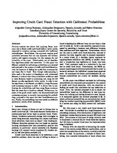
Fig. 1. The supervised samples available at day t include: i) feedbacks of the first δ days and ii) delayed couples occurred before the δ th day.
of transactions, the positive class is also called the minority class and the negative one the majority class. In general, FDSs operate on a continuous stream of transactions because frauds have to be detected online, however, the classifier is updated once a day, to gather a sufficient amount of supervised transactions. Transactions arriving at day t, namely Tt , are processed by the classifier Kt−1 trained in the previous day (t − 1). The k riskiest transactions of Tt are reported to the investigators, where k > 0 represents the number of alerts the investigators are able to validate. The reported alerts At are determined by ranking the transactions of Tt according to the posterior probability PKt−1 (+|x), which is the estimate, returned by Kt−1 , of the probability for x to be a fraud. The set of reported alerts at day t is defined as At = {x s.t. r(x) ≤ k} (1) where r(x) ∈ {1, . . . , #Tt } is the rank of the transaction x according to PKt−1 (+|x), and #(·) denotes the cardinality of a set. In other terms, the transaction with the highest probability ranks first (r(x) = 1) and the one with the lowest probability ranks last (r(x) = #Tt ). Investigators will then provide feedbacks Ft about the alerts in At , defining a set of k supervised couples (x, y) Ft = {(x, y), x ∈ At },
(2)
which represents the only immediate information that the FDS receives. At day t, we also receive the labels of all the transactions processed at day t − δ, providing a set of delayed supervised couples Dt−δ = {(x, y), x ∈ Tt−δ }, see Figure 1. Though these transactions have not been personally checked by investigators, they are by default assumed to be genuine after δ days, as far as customers do not report frauds. 1 As a result, the labels of all the transactions older than δ days are provided at day t. The problem of receiving delayed labels is also referred to as verification latency [27]. It is worth to remark that this is still a simplified description of the processes regulating companies analyzing credit cards transactions. For instance, it is typically not possible 1 Investigators typically assume that frauds missed by the FDS are reported by customers themselves (e.g. after having checked their credit card balance), within a maximum time-interval of δ days.
Fig. 2. Everyday we have a new set of feedbacks (Ft , Ft−1 , . . . , Ft−(δ−1) ) from the first δ days and a new set of delayed transactions occurred on the δ th day (Dt−δ ). In this Figure we assume δ = 7 and the colours refer to the notation in Figure 1.
to extract the alerts At by ranking the whole set Tt , since transactions have to be immediately passed to investigators; similarly, delayed supervised couples Dt−δ do not come all at once, but are provided over time. Notwithstanding, we deem that the most important aspects of the problem (i.e. the alert-feedback interaction and the time-varying nature of the stream) are already contained in our formulation and that further details would unnecessarily make the problem setting complex. Feedbacks Ft can either refer to frauds (correct alerts) or genuine transactions (false alerts): correct alerts are the true positives (TP), while false alerts are the false positives (FP). Similarly, Dt−δ contains both fraud (false negative) and genuine transactions (true negatives), although the vast majority of transactions belong to the genuine class. Figure 2 illustrates the two types of supervised pairs that are provided everyday. The goal of a FDS is to return accurate alerts: when too many FPs are reported, investigators might decide to ignore forthcoming alerts. Thus, what actually matters is to achieve the highest precision in At . This precision can be measured by the quantity pk (t) =
#{(x, y) ∈ Ft s.t. y = +} k
(3)
where pk (t) is the proportion of frauds in the top k transactions with the highest likelihood of being frauds ([4]). IV. L EARNING STRATEGY The fraud-detection scenario described in Section III suggests that learning from feedbacks Ft is a different problem than learning from delayed samples in Dt−δ . The first difference is evident: Ft provides recent, up-to-date, information while Dt−δ might be already obsolete once it comes. The second difference concerns the percentage of frauds in Ft and Dt−δ . While it is clear that the class distribution in Dt−δ is always skewed towards the genuine class (see Figure 2), the number of frauds in Ft actually depends on the performance of classifier Kt−1 : values of pk (t) ∼ 50% provide feedbacks Ft where frauds and genuine transactions are balanced, while high precision values might even result in Ft skewed towards
All%fraudulent%transac9ons%of%a%day% All%genuine%transac9ons%of%a%day% Fraudulent%transac9ons%in%the%feedback% Genuine%transac9ons%in%the%feedback%
frauds. The third, and probably the most subtle, difference is that supervised couples in Ft are not independently drawn, but are instead selected by Kt−1 among those transaction that are more likely to be frauds. As such, a classifier trained on Ft learns how to label transactions that are most likely to be fraudulent, and might be in principle not precise on the vast majority of genuine transactions. Therefore, beside the fact that Ft and Dt−δ might require different resampling methods, Ft and Dt−δ are also representative of two different classification problems and, as such, they have to be separately handled. In the following, two traditional fraud-detection approaches are presented (Section IV-A), and further developed to handle separately feedbacks and delayed supervised couples (Section IV-B). Experiments in Section V show that this is a valuable strategy, which substantially improves the alert precision.
Time%
Dt−8
Dt−7 Ft−6 Ft−5 Ft−4 Ft−3 Ft−2 Ft−1 Ft
WtD
Dt−8
Wt
Sliding' window'
Ft
Dt−7 Ft−6 Ft−5 Ft−4 Ft−3 Ft−2 Ft−1 Ft
Ensemble' M2
M1
EtD
Ft
Et
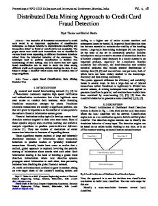
Fig. 3. Supervised information used by different classifiers in the ensemble and sliding window approach. The Figure assume that feedbacks are provided for the first 7 days (δ = 7) and delayed samples of two days before the feedbacks are available (α = 2).
A. Conventional Classification Approaches in FDS During operation, feedbacks Ft and delayed supervised samples Dt−δ can be exploited for training or updating the classifier Kt . In particular, we train the FDS considering the feedbacks from the last δ days (i.e. {Ft , Ft−1 , . . . , Ft−(δ−1) }) and the delayed supervised pairs from the last α days before the feedbacks, i.e. {Dt−δ , . . . , Dt−(δ+α−1) } (see Figure 2). 2 In the following we present two conventional solutions for concept-drift adaptation [34], [20] built upon a classification algorithm proving an estimate of the probability P (+|x). • Wt : a sliding window classifier that is daily updated over the supervised samples received in the last δ + α days, i.e. {Ft , . . . , Ft−(δ−1) , Dt−δ , . . . , Dt−(δ+α−1) } (see Figure 3). • Et : an ensemble of classifiers {M1 , M2 , . . . , Mα , F }, where Mi is trained on Dt−(δ+i−1) and Ft is trained on all the feedbacks of the last δ days {Ft , . . . , Ft−(δ−1) }. The estimate of posterior probability PEt (+|x) is estimated by averaging the posterior probabilities of the individual classifiers, PMi (+|x), i = 1, . . . , α and PFt (+|x). Note that we use a single classifier to learn from the set of feedbacks since their size is typically small. Everyday, Ft is re-trained considering the new feedbacks, while a new classifier is trained on the new delayed supervised couples provided (Dt−δ ) and included in the ensemble. At the same time, the most obsolete classifier is removed from the ensemble. These solutions implement two basic approaches for handling concept drift that can be further improved by adopting dynamic sliding windows or adaptive ensemble sizes [17]. B. Separating delayed Supervised Samples from Feedbacks Our intuition is that feedbacks and delayed transactions have to be treated separately because, beside requiring different tools for handling class unbalance, they refer to different classification problems. Therefore, at day t we 2 There
is no point of storing feedbacks from Ft−δ (or before), as these supervised couples are provided in Dt−δ (or before).
train a specific classifier Ft on the feedbacks of the last δ days {Ft , . . . , Ft−(δ−1) } and denote by PFt (+|x) its posterior probability. We then train a second classifier on the delayed samples by means either of a sliding-window or an ensemble mechanism (see Figure 3): Let us denote by WtD the classifier trained on a sliding window of delayed samples {Dt−δ , . . . , Dt−(δ+α−1) } and by PWtD (+|x) its posterior probabilities, while EtD denotes the ensemble of α classifiers {M1 , M2 , . . . , Mα } where each individual classifier Mi is trained on Dt−δ−i , i = 1, . . . , α. Then, the posterior probability PEtD (+|x) is obtained by averaging the posterior probabilities of the individual classifiers. Each of these two classifiers has to be aggregated with Ft to exploit information provided by feedbacks. However, to raise alerts, we are not interested in aggregation methods at the label level but rather at the posterior probability level. For the sake of simplicity we adopt the most straightforward combination approach based on averaging the posterior probabilities of the two classifiers (Ft and one among WtD and D EtD ). Let us denote by AE t the aggregation of Ft and Et where PAE (+|x) is defined as: t PAE (+|x) = t
PFt (+|x) + PEtD (+|x) 2
(4)
Similar definition holds for the aggregation of Ft and WtD D (AW t ). Note that Ft and Wt jointly use the training set of Wt and, similarly, the two classifiers Ft and EtD jointly use the same training samples of Et (see Figure 3). However, in Wt feedbacks represent a small portion of the supervised samples used for training, hence they have little influence on PWt (+|x), while in the aggregation AW t their contribution becomes more prominent. Similarly, Ft represents one of the classifiers of the ensemble Et , hence it has in principle the same influence as all the other α classifiers trained on delayed samples to determine PEt (+|x).3 . 3 In the specific case of the ensemble and of posterior probabilities computed by averaging (4), the aggregation of Ft and EtD (AE t ) corresponds to assigning a larger weight to Ft in Et .
TABLE I DATASETS Id 2013 2014
Start day 2013-09-05 2014-08-05
End day 2014-01-18 2014-10-09
# Days 136 44
# Instances 21,830,330 7,619,452
# Features 51 51
% Fraud 0.19% 0.22%
Experiments in Section V show that handling feedbacks separately from delayed supervised samples provides much more precise alerts, and that FDSs relying on classifiers trained exclusively on feedbacks and delayed supervised E samples (like AW t and At ) substantially outperform FDSs trained on feedbacks and delayed supervised samples pooled together (like Wt and Et ). In what follows, as practical example of the separation of feedbacks from delayed supervised couples, we detail the specific solutions based on Random Forests that were used in our experiments. C. Two Specific FDSs based on Random Forest As a base algorithm the FDSs presented in the previous section we used a Random Forest [9] with 100 trees. In particular, for WtD , Wt and for all Mi , i = 1, . . . , α, we used a Balanced Random Forest (BRF) where each tree is trained on a balanced bootstrap sample, obtained by randomly undersampling the majority class while preserving all the minority class samples in the corresponding training set. Each tree of BRF receives a different random sample of the genuine transactions and the same samples from the fraud class in the traininig set, yielding a balanced training set. This undersampling strategy allows one to learn trees with balanced distribution and to exploit many subsets of the majority class. At the same time, this resampling method reduces training sizes and improve detection speed. A drawback of undersampling is that we are potentially removing relevant training samples form the dataset, however this problem is mitigated by the fact that we learn 100 different trees. Using undersampling allows us to rebalance the batches without propagating minority class observations along the streams as in [20]. Propagating frauds between batches should be avoided whenever possible, since it requires access to previous batches that we might not be able to store when data arrives in streams. In contrast, for Ft that is trained on feedbacks we adopted a standard Random Forest (RF) where no resampling is performed. V. E XPERIMENTS We considered two datasets of credit card transactions of European cardholders: the first one (referred to as 2013) is composed of daily transactions from the 5th of September 2013 to the 18th of January 2014, the second one (referred to as 2014) contains transactions from the 5th of August to the 9th of September 2014. In the 2013 dataset there is an average of 160k transactions per day and about 304 frauds per day, while in the 2014 dataset there is on average 173k transactions and 380 frauds everyday. Table I reports few additional details about these datasets and shows that they are also heavily unbalanced.
In the first experiments we process both datasets to assess the importance of separating feedbacks from delayed supervised samples. Though we expect these streams to be affected by concept drift (CD), since they span a quite long time range, we do not have any ground truth to investigate the reaction to concept drift of the proposed FDS. To this purpose, we design the second experiment where we juxtapose batches of transactions acquired in different times of the year to artificially introduce CD in a specific day in the transaction stream. In both experiments we test FDSs built on random forests presented in Section IV-C. We considered both the sliding window and ensemble approaches and compared the accuracy of pooling feedbacks and delayed supervised samples together (Wt and Et ) against learning separate classifiers (Ft , E WtD and EtD ) that are then aggregated (AW t and At ). Let us recall that alerts are raised by each tested classifier. This means that also the feedbacks returned to the classifiers might be different. This has to be considered when comparing different classifiers, for instance, when comparing Wt and WtD , the supervised information provided is not the same because, in the first case alerts are raised by Wt while in the second by WtD . We assume that after δ = 7 days all the transactions labels are provided (delayed supervised information) and that we have a budget of k = 100 alerts that can be checked by the investigators: thus, Ft is trained on a window of 700 feedbacks. We set α = 16 so that WtD is trained on a window of 16 days and EtD (resp. Et ) is an ensemble of 16 (resp. 17) classifiers. 4
Each experiments is repeated 10 times to reduce the results’ variability due to bootstrapping of the training sets in the random forests. The FDS performance is assessed by means of the average pk over all the batches (the higher the better) and use a paired t-test to assess whether the performance gaps between each pair of tested classifiers is significant or not. We compute the paired t-test on the ranks resulting from the Friedman test [18] as recommended by Demsar [14]. In practice, for each batch, we rank the strategies from the least to the best performing and then compare each strategy against the others by means of a paired t-test based on the ranks. Then we sum the ranks over all batches. More formally, let rs,j ∈ {1, . . . , S} be the rank of strategy s on day j and S be the number of strategies to compare. The strategy with the highest accuracy in j has rs,j = S and the one with the lowest has rs,j = 1. The paired t-test compares ranks of strategy a against b by means of ra,j − rb,j , j ∈ {1, . . . , J}, where J is the total number of P batches. Then the sum of ranks for strategy s is defined J as j=1 rj,s . The higher the sum, the higher is the number of times that one strategy is superior to the others.
4 We ran several experiments with α = 1, 8, 16, 24 and found α = 16 as a good trade-off between performance, computational load, and the number of days that can be used for testing in each stream.
A. Experiments on 2013 and 2014 Datasets In order to evaluate the benefit of learning on feedbacks and delayed samples separately, we first compare the performance of classifier Wt against Ft , WtD and the aggregation AW t . Table II shows the average pk over all the batches for the two datasets separately. In both 2013 and TABLE II AVERAGE pk BETWEEN ALL THE BATCHES
classifier F WD W AW
Dataset mean 0.609 0.540 0.563 0.697
2013 sd 0.250 0.227 0.233 0.212
Dataset mean 0.596 0.549 0.559 0.657
2014 sd 0.249 0.253 0.256 0.236
2014 datasets, AW t outperforms the other FDSs in terms of pk . The barplots of Figure 5 show the sum of ranks for each classifier and the results of the paired t-tests. Figure 5 indicates that in both datasets (Figures 5(a) and 5(b)) AW t is significantly better than all the other classifiers. Ft achieves higher average pk and higher sum of ranks than WtD and Wt : this confirms that feedbacks are very important to increase pk . Figure 4(a) displays the value of pk for AW t and Wt in each day, averaged in a neighborhood of 15 days. During December there is a substantial performance drop, that can be seen as a Concept Drift (CD) due to a change in cardholder behaviour before Christmas. However, AW t dominates Wt along the whole 2013 dataset, which confirms that a classifier AW t that learns on feedbacks and delayed transactions separately outperforms a classifier Wt trained on all the supervised information pooled together (feedbacks and delayed transactions). Figures 5(c), 5(d) and Tables III confirm this claim also when the FDSs implements an ensemble of classifiers. 5 In particular, Figure 4(b) displays the smoothed average pk of E classifiers AE t and Et . For the whole dataset At has better pk than Et . TABLE III AVERAGE pk BETWEEN ALL THE BATCHES
classifier F ED E AE
Dataset mean 0.603 0.459 0.555 0.683
2013 sd 0.258 0.237 0.239 0.220
Dataset mean 0.596 0.443 0.516 0.634
2014 sd 0.271 0.242 0.252 0.239
B. Experiments on artificial dataset with CD In this section we artificially introduce an abrupt CD in specific days by juxtaposing transactions acquired in different times of the year. Table IV reports the three datasets that have been generated by concatenating batches of the dataset 2013 with batches from 2014. The number of days after concept 5 Please note that classifier F returns different results between Table II t and Table III because of the stochastic nature of RF.
AE E
AW W
(a) Sliding window strategies
(b) Ensemble strategies
Fig. 4. Average pk per day (the higher the better) for classifiers on dataset 2013 smoothed using moving average of 15 days. In the sliding window approach classifier AW t has higher pk than Wt , and in the ensemble approach AE t is superior than Et .
drift is set such that the FDS has the time to forget the information from the previous concept. TABLE IV DATASETS WITH A RTIFICIALLY I NTRODUCED CD Id CD1 CD2 CD3
Start 2013 2013-09-05 2013-10-01 2013-11-01
End 2013 2013-09-30 2013-10-31 2013-11-30
Start 2014 2014-08-05 2014-09-01 2014-08-05
End 2014 2014-08-31 2014-09-30 2014-08-31
Table V(a) shows the values of pk averaged over all the batches in the month before the change for the sliding window approach, while Table V(b) shows pk in the month reports the highest pk before and after after the CD. AW t CD. Similar results are obtained with the ensemble approach TABLE V AVERAGE pk IN THE MONTH BEFORE AND AFTER CD FOR THE SLIDING WINDOW APPROACH
(a) Before CD classifier F WD W AW
CD1 mean sd 0.411 0.142 0.291 0.129 0.332 0.215 0.598 0.192
classifier F WD W AW
CD1 mean sd 0.635 0.279 0.536 0.335 0.570 0.309 0.714 0.250
CD2 mean sd 0.754 0.270 0.757 0.265 0.758 0.261 0.788 0.261
CD3 mean sd 0.690 0.252 0.622 0.228 0.640 0.227 0.768 0.221
(b) After CD CD2 mean sd 0.511 0.224 0.374 0.218 0.391 0.213 0.594 0.210
CD3 mean sd 0.599 0.271 0.515 0.331 0.546 0.319 0.675 0.244
(Tables VI(a), VI(b)). In all these experiments, AE t is also faster than standard classifiers Et and Wt to react in the presence of a CD (see Figure 6). The large variation of pk over the time reflect the non-stationarity of the data stream. Expect for dataset CD1, we have on average lower pk after concept drift. C. Discussion In this section we analyze the accuracy improvements E achieved by classifiers AW t and At proposed in Section IVB. First of all, we notice that the classifier learned on recent feedbacks is more accurate that the one learned on delayed samples. This is made explicit by Tables II and III showing that Ft often outperforms WtD (and EtD ), and Wt (and Et ).
AW
F
W
WD
AW
F
W
WD
AE
F
E
ED
AE
F
E
ED
(a) Sliding window strategies on (b) Sliding window strategies on (c) Ensemble strategies on dataset (d) Ensemble strategies on dataset dataset 2013 dataset 2014 2013 2014 Fig. 5. Comparison of classification strategies using sum of ranks in all batches and paired t-test based upon on the ranks of each batch (classifiers having E the same letter on their bar are not significantly different with a confidence level of 0.95). In both datasets (2013 and 2014), classifiers AW t and At are significantly better that the others.
AW W
AW W
AW W
AE E
(a) Sliding window strategies on (b) Sliding window strategies on (c) Sliding window strategies on (d) Ensemble strategies on dataset dataset CD1 dataset CD2 dataset CD3 CD3 Fig. 6. Average pk per day (the higher the better) for classifiers on datasets with artificial concept drift (CD1, CD2 and CD3) smoothed using moving E average of 15 days. In all datasets AW t has higher pk than Wt . For the ensemble approach we show only dataset CD3, where At dominates Et for the whole dataset (similar results are obtained on CD1 and CD2, but they are not included for compactness). The vertical bar denotes the date of the concept drift. TABLE VI AVERAGE pk IN THE MONTH BEFORE AND AFTER CD FOR THE ENSEMBLE APPROACH
(a) Before CD classifier F ED E AE
CD1 mean sd 0.585 0.183 0.555 0.318 0.618 0.313 0.666 0.222
classifier F ED E AE
CD1 mean sd 0.696 0.270 0.551 0.298 0.654 0.266 0.740 0.232
CD2 mean sd 0.731 0.267 0.563 0.217 0.696 0.276 0.772 0.272
CD3 mean sd 0.706 0.245 0.562 0.223 0.648 0.245 0.751 0.221
(b) After CD CD2 mean sd 0.477 0.235 0.286 0.182 0.373 0.235 0.575 0.227
CD3 mean sd 0.610 0.270 0.486 0.265 0.581 0.268 0.659 0.245
We deem that Ft outperforms WtD (resp. EtD ) since WtD (resp. EtD ) are trained on less recent supervised couples. As far as the improvement with respect to Wt (and Et ) is concerned, our interpretation is that this is due to the fact that Wt (and Et ) are trained on the entire supervised dataset, then weakening the specific contribution of feedbacks. Our results instead show that aggregation prevents the large amount of delayed supervised samples to dominate the small set of immediate feedbacks. This boils down to assign larger weights to the most recent than to the old samples, which is a golden rule when learning in non-stationary environments. The aggregation AW t is indeed an effective way
to attribute higher importance to the information included in the feedbacks. At the same time AE t is a way to balance the contribution of Ft and the remaining α models of Et . Another motivation of the accuracy improvement is that classifiers trained on feedbacks and delayed samples address two different classification tasks (Section IV). For this reason too, it is not convenient to pool the two types of supervised samples together. Finally, the aggregation presented in equation 4 provides equal weights to the two posterior probabilities PFt and PWtD (PEtD ). However, more sophisticated and eventually adaptive aggregation schemes (e.g. non-linear or stacking [8]) could be used to react to concept drift. In fact, in a rapidly drifting environment, the relative weight of PFt should eventually increase, because WtD (or EtD ) might be obsolete and prone to false alarms. VI. C ONCLUSION In this paper we formalise a framework that reproduces the working conditions of real-world FDSs. In a realworld fraud-detection scenario, the only recent supervisedinformation is provided on the basis of the alerts generated by the FDS and feedbacks provided by investigators. All the other supervised samples are provided with a much larger delay. Our intuition is that the alert-feedback interaction has to be explicitly considered to improve alert precision and that feedbacks and delayed samples have to be separately
handled when training a realistic FDS. To this purpose, we have considered two general approaches for fraud detection: a sliding window and an ensemble of classifiers. We have then compared FDSs that separately learn on feedbacks and delayed samples against FDSs that pool all the available supervised information together. Experiments run on realworld streams of transactions show that the former strategy provides much more precise alerts than the latter, and that it also adapts more promptly in concept-drifting environments. Future work will focus on investigating adaptive mechanisms to aggregate the classifier trained on feedbacks and the one trained on delayed samples, to further improve the alert precision in non-stationary streams. R EFERENCES [1] E. Aleskerov, B. Freisleben, and B. Rao. Cardwatch: A neural network based database mining system for credit card fraud detection. In Computational Intelligence for Financial Engineering (CIFEr), 1997., Proceedings of the IEEE/IAFE 1997, pages 220–226. IEEE, 1997. [2] C. Alippi, G. Boracchi, and M. Roveri. Just-in-time classifiers for recurrent concepts. Neural Networks and Learning Systems, IEEE Transactions on, 24(4):620–634, April. [3] G. Batista, A. Carvalho, and M. Monard. Applying one-sided selection to unbalanced datasets. MICAI 2000: Advances in Artificial Intelligence, pages 315–325, 2000. [4] S. Bhattacharyya, S. Jha, K. Tharakunnel, and J. C. Westland. Data mining for credit card fraud: A comparative study. Decision Support Systems, 50(3):602–613, 2011. [5] R. Bolton and D. Hand. Statistical fraud detection: A review. Statistical Science, pages 235–249, 2002. [6] R. Bolton, D. Hand, et al. Unsupervised profiling methods for fraud detection. Credit Scoring and Credit Control VII, pages 235–255, 2001. [7] R. Brause, T. Langsdorf, and M. Hepp. Neural data mining for credit card fraud detection. In Tools with Artificial Intelligence, 1999. Proceedings. 11th IEEE International Conference on, pages 103–106. IEEE, 1999. [8] L. Breiman. Stacked regressions. Machine learning, 24(1):49–64, 1996. [9] L. Breiman. Random forests. Machine learning, 45(1):5–32, 2001. [10] P. Chan, W. Fan, A. Prodromidis, and S. Stolfo. Distributed data mining in credit card fraud detection. Intelligent Systems and their Applications, 14(6):67–74, 1999. [11] S. Chen and H. He. Towards incremental learning of nonstationary imbalanced data stream: a multiple selectively recursive approach. Evolving Systems, 2(1):35–50, 2011. [12] A. Dal Pozzolo, O. Caelen, Y.-A. Le Borgne, S. Waterschoot, and G. Bontempi. Learned lessons in credit card fraud detection from a practitioner perspective. Expert Systems with Applications, 41(10):4915–4928, 2014. [13] A. Dal Pozzolo, R. Johnson, O. Caelen, S. Waterschoot, N. V. Chawla, and G. Bontempi. Using hddt to avoid instances propagation in unbalanced and evolving data streams. In Neural Networks (IJCNN), The 2014 International Joint Conference on. IEEE, 2014. [14] J. Demˇsar. Statistical comparisons of classifiers over multiple data sets. The Journal of Machine Learning Research, 7:1–30, 2006. [15] G. Ditzler and R. Polikar. An ensemble based incremental learning framework for concept drift and class imbalance. In Neural Networks (IJCNN), The 2010 International Joint Conference on, pages 1–8. IEEE, 2010. [16] J. Dorronsoro, F. Ginel, C. Sgnchez, and C. Cruz. Neural fraud detection in credit card operations. Neural Networks, 8(4):827–834, 1997. [17] W. Fan. Systematic data selection to mine concept-drifting data streams. In Proceedings of the tenth ACM SIGKDD international conference on Knowledge discovery and data mining, pages 128–137. ACM, 2004. [18] M. Friedman. The use of ranks to avoid the assumption of normality implicit in the analysis of variance. Journal of the American Statistical Association, 32(200):675–701, 1937.
ˇ [19] J. Gama, I. Zliobait˙ e, A. Bifet, M. Pechenizkiy, and A. Bouchachia. A survey on concept drift adaptation. ACM Computing Surveys (CSUR), 46(4):44, 2014. [20] J. Gao, B. Ding, W. Fan, J. Han, and P. S. Yu. Classifying data streams with skewed class distributions and concept drifts. Internet Computing, 12(6):37–49, 2008. [21] J. Gao, W. Fan, J. Han, and S. Y. Philip. A general framework for mining concept-drifting data streams with skewed distributions. In SDM, 2007. [22] S. Ghosh and D. L. Reilly. Credit card fraud detection with a neuralnetwork. In System Sciences, 1994. Proceedings of the Twenty-Seventh Hawaii International Conference on, volume 3, pages 621–630. IEEE, 1994. [23] D. Hand, C. Whitrow, N. Adams, P. Juszczak, and D. Weston. Performance criteria for plastic card fraud detection tools. Journal of the Operational Research Society, 59(7):956–962, 2008. [24] H. He and E. A. Garcia. Learning from imbalanced data. Knowledge and Data Engineering, IEEE Transactions on, 21(9):1263–1284, 2009. [25] P. Juszczak, N. M. Adams, D. J. Hand, C. Whitrow, and D. J. Weston. Off-the-peg and bespoke classifiers for fraud detection. Computational Statistics & Data Analysis, 52(9):4521–4532, 2008. [26] J. Z. Kolter and M. A. Maloof. Dynamic weighted majority: An ensemble method for drifting concepts. The Journal of Machine Learning Research, 8:2755–2790, 2007. [27] G. Krempl and V. Hofer. Classification in presence of drift and latency. In Data Mining Workshops (ICDMW), 2011 IEEE 11th International Conference on, pages 596–603. IEEE, 2011. [28] R. N. Lichtenwalter and N. V. Chawla. Adaptive methods for classification in arbitrarily imbalanced and drifting data streams. In New Frontiers in Applied Data Mining, pages 53–75. Springer, 2010. [29] D. Malekian and M. R. Hashemi. An adaptive profile based fraud detection framework for handling concept drift. In Information Security and Cryptology (ISCISC), 2013 10th International ISC Conference on, pages 1–6. IEEE, 2013. [30] C. Phua, V. Lee, K. Smith, and R. Gayler. A comprehensive survey of data mining-based fraud detection research. arXiv preprint arXiv:1009.6119, 2010. [31] J. T. Quah and M. Sriganesh. Real-time credit card fraud detection using computational intelligence. Expert Systems with Applications, 35(4):1721–1732, 2008. [32] J. C. Schlimmer and R. H. Granger Jr. Incremental learning from noisy data. Machine learning, 1(3):317–354, 1986. [33] W. N. Street and Y. Kim. A streaming ensemble algorithm (sea) for large-scale classification. In Proceedings of the seventh ACM SIGKDD international conference on Knowledge discovery and data mining, pages 377–382. ACM, 2001. [34] D. K. Tasoulis, N. M. Adams, and D. J. Hand. Unsupervised clustering in streaming data. In ICDM Workshops, pages 638–642, 2006. [35] H. Wang, W. Fan, P. S. Yu, and J. Han. Mining concept-drifting data streams using ensemble classifiers. In Proceedings of the ninth ACM SIGKDD international conference on Knowledge discovery and data mining, pages 226–235. ACM, 2003. [36] D. Weston, D. Hand, N. Adams, C. Whitrow, and P. Juszczak. Plastic card fraud detection using peer group analysis. Advances in Data Analysis and Classification, 2(1):45–62, 2008. [37] C. Whitrow, D. J. Hand, P. Juszczak, D. Weston, and N. M. Adams. Transaction aggregation as a strategy for credit card fraud detection. Data Mining and Knowledge Discovery, 18(1):30–55, 2009. [38] G. Widmer and M. Kubat. Learning in the presence of concept drift and hidden contexts. Machine learning, 23(1):69–101, 1996.