Critical Bottleneck Size for Jamless Particle Flows in Two Dimensions

Critical Bottleneck Size for Jamless Particle Flows in Two Dimensions Takumi Masuda,1 Katsuhiro Nishinari,1 and Andreas Schadschneider2 1

arXiv:1403.6570v1 [cond-mat.stat-mech] 26 Mar 2014

Department of Aeronautics and Astronautics, Faculty of Engineering, University of Tokyo, Hongo, Bunkyo-ku, Tokyo 113-8656, Japan 2 Institut f¨ ur Theoretische Physik, Universit¨ at zu K¨ oln, 50937 K¨ oln, Germany (Dated: March 27, 2014) We propose a simple microscopic model for arching phenomena at bottlenecks. The dynamics of particles in front of a bottleneck is described by a one-dimensional stochastic cellular automaton on a semicircular geometry. The model reproduces oscillation phenomena due to formation and collapsing of arches. It predicts the existence of a critical bottleneck size for continuous particle flows. The dependence of the jamming probability on the system size is approximated by the Gompertz function. The analytical results are in good agreement with simulations. PACS numbers: 89.75.Fb, 45.70.-n, 89.40.-a, 02.50.Ey, 05.65.+b

Granular materials are many-particle systems that display interesting and unintuitive physical properties [1, 2]. One of their most important types of behavior is formation of arches which leads to a mutual arrest of their constituent particles in front of a bottleneck. Such situation is usually called a ”jam”. Usually it is an undesirable state since it causes many problems, e.g., in industrial applications. It often occurs in systems such as traffic [3], granular flow through a hopper [4] and escaping stampedes during evacuations [5]. Cates et al., in their comprehensive study [6], suggest that jammed systems should be categorized as a new class ”fragile matter”, i.e. materials which respond to applied stress by reorganizing their internal structures through force chains. Liu and Nagel [7] extend the concept not only to grains, bubbles and droplets but also to glass transitions. One focus of recent studies on granular flows has been on bottleneck flows with external perturbations, e.g., vibrations. Vibrated granular flows exhibit intermittent behavior, which reflects phase transitions between a jamming and an unjamming state. Several experiments have revealed properties of granular flows through a bottleneck. The most important one is the existence of a critical outlet size above which no arches appear [4]. However, some empirical laws do not determine the critical outlet size [8]. In addition, the two states of intermittent flows alternate randomly and lifetime distributions have been investigated. The avalanche size, defined as the number of grains passing through a bottleneck during a single unjamming state, follows an exponential distribution [8–12]. On the other hand, the duration of an unjamming state obeys power law and its expectation value does not converge for low magnitudes of vibration [11]. In some situations, pedestrian crowds exhibit collective phenomena similar to those in granular materials, e.g., lane formation as in oppositely charged colloids [13] and for evacuation flows at bottlenecks [5, 14]. The latter shows very similar behavior to a granular flow since also in pedestrian crowds formation and collapsing of

arches has been observed. Although granular materials require external perturbations to resume flows, pedestrian crowds rapidly destroy clogging by self-adjustment. In the following we propose a simple model that captures the essence of the observed behavior of manyparticle systems near a bottleneck, e.g., oscillation phenomena. Although particle flows usually are threedimensional, we focus here on two-dimensional realizations which are relevant for pedestrian dynamics, but have also been studied for granular materials. For simplicity, we ignore fluctuations that occur in the bulk of granular assemblies [10]. Instead, we focus on properties of intermittent behavior which stem from arching phenomena. The precise structure of the arches is not relevant for the properties of the flow. This assumption allows us to formulate the dynamics of the particles by a one-dimensional stochastic cellular automaton. Its sites are arranged in a semicircular shape which reflects the typical form of arches (Fig. 1). Here we have assumed that no arches appear in the area nearer to the bottleneck than the semicircle, which implies that its size is of the order of the bottleneck width. If the site size is chosen as the typical size of the particles (grains), each site can be occupied by at most one particle. Hence, each site j can be in two different states, empty (sj = 0) or occupied (sj = 1). The configuration (1, . . . , 1) where all sites are occupied represents arch formation. If P (C) denotes the probability of finding a configuration C = (s1 , . . . , sL ) in the steady state, the arching probability is given by Parch = P (1, . . . , 1). In order to define the dynamics of the model we assume that the bulk of the granular assembly acts as a particle bath which supplies particles to the system at a constant rate α. Then empty sites become occupied with the probability of α which can be interpreted as the probability that a particle finds an available gap. It is called ”inflow” in the following. The ”outflow” is represented by the annihilation of a particle. The probability of this process depends on the occupancy of the two neighboring sites. If both are occupied, then the particle is annihi-

2

γ,δ N ) is given by Qarch (1 − Qarch )t−(N +1) which has the expectation value 1/Qarch + N . For simplicity, we restrict our attention to the cases where α = β 6= 0 and γ = δ. The first condition implies that inflow and outflow rates are identical when no friction acts. The second identity implies that the friction

The cumulative number of 'outflow'

exit

between particles and between particles and walls are identical. In this situation, Qarch is independent of the system size L. We introduce a new parameter ε = γ/α so that 0 ≤ ε ≤ 1 in the physical regime. We first consider two limiting cases. In the case ε = 0, flow cannot resume once an arch has formed. This situation corresponds to an absorbing state where the system attains a trivial stationary state without dynamics. Similar behavior is observed when granular materials flow through a narrow hopper without vibration. When ε = 1, all configurations appear uniformly in the steady state since inflow and outflow occur at the same rate. Therefore the probability for each configuration is 1/2L . We can interpret the parameter ε as an indicator for the magnitude of destabilization of arches since the conditions ε = 0 and ε = 1 correspond to jamming and continuous flow, respectively. Additionally, ε accounts for arch destabilization by pedestrians. Consider a situation where arches are formed during a rush through a bottleneck. Because of the high velocity of the pedestrians and the large friction between them this situation is described by large values of α and β and small values of γ and δ. As a consequence, ε is small and can be viewed as an indicator for the pedestrian’s discipline near the exit. 40 35 30 25 20 15 10 5 0 0

25

50

75

100 125 150 175 200

time step

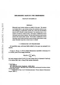
FIG. 2. The dynamical behavior of the model for α = β = 0.9, γ = δ = 0.1, L = 3 and different realizations of the stochastic dynamics. The vertical axis indicates the cumulative number of outflowing (annihilated) particles.

The collective behavior observed in simulations is in good qualitative agreement with experiments on granular materials. The dynamical behavior of the model indicates the presence of two states: jamming and continuous flow. Jamming is represented in the graph (Fig. 2) by horizontal regions, where due to the existence of an arch no particles are annihilated. The other parts show nonvanishing particle flows. A similar intermittent behavior with random alternation between two such states can be observed in granular flows and escaping stampedes [11, 14]. Let us now focus on the avalanche size m. In our model, the avalanche size is defined as the number of outflowing particles between two successive ”stable” arches. Presuming that avalanche sizes are distributed exponen-

3 tially as observed in experiments, we are interested in their expectation value alone. It is obtained by dividing the number of outflowing particles per unit time by the number of avalanches. The latter is identical to the number of stable arches since they occur alternately. Therefore, it is given by SParch Qarch where Parch Qarch = Parch /(1/Qarch) is the number of arches per unit time. In addition, the number of outflowing particles per unit time is obtained as weighted average of flow rates for configurations on their distribution. Introducing 2L -dimensional vectors |P i and hQ| such that X P (s1 , . . . , sL )|s1 , . . . , sL i, (1) |P i =

|P i is given by |P i =

X

Q(s1 , . . . , sL )hs1 , . . . , sL |

(2)

hw|P i =

R(ε, L) =

    1 0 , |1i = , 0 1

we can write P the weighted average as hQ|P i . The summation (s1 ,...,sL ) is over all configurations. Thus the expectation value of avalanche sizes m is represented as 1 m= SR(ε, L)

Qarch Parch where R(ε, L) = . hQ|P i

(3)

The form of (3) implies that the variables (γ, ε, L, N ) of m are separated so that R(ε, L) depends only on physical properties of the system and S contains parameters (γ, N ) which do not have a simple interpretation in real systems. Since (γ, N ) depend on the length of the time step they have to be determined empirically for each experiment. In the following, we consider the distribution of configurations in the steady state |P i to represent (3) in an explicit form. Its time evolution is given by the master equation. Using the quantum formalism (see e.g., [15, 16]), it can be cast in the form of a Schr¨odinger equation with some ”Hamiltonian” H defined by the transition rates. In the stationary state it takes the form H|P i = 0 .

(4)

The Hamiltonian is readily constructed from the update rule of the model. Because of the 3-site interaction the Hamiltonian of our model is more complicated than e.g., the asymmetric exclusion process. We readily deduce det H = 0 since the master equation implies that H has an eigenvalue 0. From the general relation H(adjH)|vi = (det H)|vi = 0, where |vi is an arbitrary vector, it follows that the formal solution of P (4) is (adjH)|vi. We choose |vi as the vector |V i = (s1 ,...,sL ) |s1 , . . . , sL i. We will show elsewhere that the choice of |vi does not depend on the form of H.

(6)

det[ H + |V ih1, · · · , 1| ] . det[ H + |V ihQ|/Qarch ]

(7)

We emphasize that the result (6) is exact and holds for any stochastic cellular automaton model with finite number of sites. 0

10

-1

10 Relative frequency

|s1 , · · · , sL i = |s1 i ⊗ · · · ⊗ |sL i, |0i =

det[ H + |V ihw| ] . det[ H + |V ihV | ]

By using (6), R(ε, L) is given by

(s1 ,...,sL )

where

(5)

The denominator of |P i is the normalization constant for the conservation of probabilities. After a cumbersome calculation, we obtain a simpler form of hw|P i where hw| is an arbitrary vector:

(s1 ,...,sL )

hQ| =

(adj H)|V i . hV |(adj H)|V i

-2

10

-3

10

10-4 10-5 10-6 10-7

0

200

400 600 Avalanche size

800

1000

FIG. 3. Histogram of avalanche sizes. The dotted line is calculated with (3) under the presumption that the distribution is exponential. Dots are simulation results for α = β = 0.7, γ = δ = 0.3, L = 4, and N = 10.

As shown in Fig. 3, the simulation results agree well with the presumption that avalanche sizes in our model are distributed exponentially. The exponential distribution of avalanche sizes has also been observed in experiments and other simulations of granular flow [8, 9, 11]. Let us now consider the jamming probability J. It is interpreted in our model as the probability that an avalanche size is less than a threshold M . Hence, it is obtained by integrating the avalanche size distribution from 0 to M : J =1 − exp(−M/m) = 1 − exp[−SM R(ε, L)].

(8)

Although the dependence of R(ε, L) on ε has a rational form as implied from (7), the dependence on L is nontrivial. This fact motivates us to approximate R(ε, L) by an analytical function. Figure. 4 shows that R(ε, L) is represented by an exponential function A(ε) exp[−B(ε)L] for ε ≥ 0.5. In fact, this assumption can be justified for the case ε = 1. Identifying A(ε) and B(ε) with R(ε, 3) and

4

R(ε,L)

10

0

10

-1

10

-2

10-3 10

ε 0.1 0.3 0.5 0.7 0.9

-4

10-5 10

-6

2

4

6

8

10

12

14

16

18

20

System size L

FIG. 4. Dependence of R(ε, L) on L. The dots correspond to simulation results for different values of ε. The lines are fixed by the two points R(ε, 3) and R(ε, 4) for corresponding ε. It is found that for ε ≥ 0.5. R(ε, L) can be approximated by an exponential function.

R(ε, 4), we can write the jamming probability with the Gompertz function as J(ε, L) =1 − exp[−A(ε)SM exp[−B(ε)L] ], 4

A(ε) =R(ε, 3) R(ε, 4)

−3

,

(9) (10)

B(ε) = log R(ε, 3) − log R(ε, 4).

(11)

R(ε, 3) and R(ε, 4) are calculated from (7) as ε + 23 , 4(7ε + 17) 11ε2 + 78ε + 103 R(ε, 4) = . 2(24ε3 + 181ε2 + 366ε + 197) R(ε, 3) =

(12) (13)

Jamming probability J

The simulation results shown in Fig. 5 agree well with our previous assumptions that the avalanche size distribution and R(ε, L) are exponential. 1 0.9 0.8 0.7 0.6 0.5 0.4 0.3 0.2 0.1 0

M 1000 5000 10000 50000 100000

0

2

4

6

8

10 12 14 16 18 20

System size L

FIG. 5. Jamming probabilities as functions of system size. The plots are simulation results and the lines are defined by (9). The jamming probabilities gradually decrease with increasing system size. They practically become zero already for relatively small system size. The system parameters are α = β = 0.45, γ = δ = 0.4 and N = 10.

The jamming probability J converges to 1 for any system size in the limit M → ∞ in principle, as deduced from (9). However, at a finite M the jamming probability becomes 0 at a finite system size L in practice. In

experiments, this fact corresponds to the existence of a critical outlet size above which no arches appear [4, 8]. A typical value of ε may be estimated from experimental results. In [12], Mankoc et al. introduced the bivariate model characterized by p and q, which indicate the probability that a particle passes through the outlet without forming an arch and the probability that a particle is delivered from an arch respectively. The parameters have been experimentally estimated as p = 0.981, q = 0.836 for an outlet of 3.02 grain diameters width. Although their experiments are in three- dimensions, we assume that the results are appropriate for our model. From the definition, q can be interpreted in our model as S = 1 − q. Comparing the expectation values of avalanche sizes deduced by both models, we obtain that R(ε, L) = (1 − p)/(p + q − pq). Additionally, we use L ≃ 6.9 which is reported from experiments in [17] as the number of particles involved in an arch for the outlet of 3.03 grains diameter width. Then we obtain ε ≃ 0.92. We interpret the dynamical behavior of particles in front of a bottleneck as the cellular automaton model with 3-site interactions arranged in a semicircular shape. From the simulations and the analytical results we can conclude that the model reproduces the generic behavior which characterizes bottleneck flows in many-particle systems. The resulting dynamics exhibits two clear regions: jamming and continuous flow. The avalanche size distribution is exponential and the jamming probability is well approximated by the Gompertz function. The expectation value of avalanche sizes and the coefficients of the Gompertz function can be determined analytically. The model reveals the existence of a critical outlet size above which no arches appear in practice. The parameter ε, which characterizes the physical properties of the model, can be estimated by methods which have been used in previous studies. The model can be extended to be more compatible with actual particle flows. Although we focus on twodimensional flows for simplicity, the model can be extended to three-dimensional flows in a straightforward way. Moreover, we have formulated the model assuming that an arch appears only in a single semicircular layer. Again the model can be made more realistic by considering multiple layers to take into account the effects of the upstream and allow for variations in arch size.

[1] A. Mehta, Granular Matter: An Interdisciplinary Approach (Springer-Verlag New York, 1994). [2] I. S. Aranson and L. S. Tsimring, Rev. Mod. Phys. 78, 641 (2006). [3] D. Chowdhury, L. Santen, and A. Schadschneider, Phys. Rep. 329, 199 (2000). [4] K. To, P-Y. Lai, and H. K. Pak, Phys. Rev. Lett. 86, 71 (2001).

5 [5] D. Helbing, I. Farkas, and T. Vicsek, Nature (London) 407, 487 (2000). [6] M. E. Cates, J. P. Wittmer, J.-P. Bouchaud, and P. Claudin, Phys. Rev. Lett. 81, 1841 (1998). [7] A. J. Liu and S. R. Nagel, Nature (London) 396, 21 (1998). [8] A. Janda, I. Zuriguel, A. Garcimart´ın, L. A. Pugnaloni, and D. Maza, Europhys. Lett. 84, 44002 (2008). [9] I. Zuriguel, A. Garcimart´ın, D. Maza, L. A. Pugnaloni, and J. M. Pastor, Phys. Rev. E 71, 051303 (2005). [10] D. Helbing, A. Johansson, J. Mathiesen, M. H. Jensen, and A. Hansen, Phys. Rev. Lett. 97, 168001 (2006). [11] A. Janda, D. Maza, A. Garcimart´ın, E. Kolb, J. Lanuza, and E. Cl´ement, Europhys. Lett. 87, 24002 (2009). [12] C. Mankoc, A. Garcimartin, I. Zuriguel, D. Maza, and

L. A. Pugnaloni, Phys. Rev. E 80, 011309 (2009). [13] T. Visser, A. Wysocki, M. Rex, H. L¨ owen, C.P Royall, A. Imhof, and A. van Blaaderen, Soft Matter 7, 2352 (2011). [14] D. Helbing, L. Buzna, A. Johansson, and T. Werner, Transp. Sci. 39, 1 (2005). [15] G. M. Sch¨ utz, in Phase Transportions and Critical Phenomena, edited by C. Domb and J. L. Lebowitz (Academic Press, New York, 2001), Vol. 19. [16] A. Schadschneider, D. Chowdhury, and K. Nishinari, Stochastic Transport in Complex Systems: From Molecules to Vehicles, (Elsevier, Amsterdam, 2010) [17] A. Garcimart´ın, I. Zuriguel, L. A. Pugnaloni, and A. Janda Phys. Rev. E 82, 031306 (2010).