May 3, 2014 - coprime integers, we construct an infinite family of Robin boundary ..... that the triangle (3.3) reduces to a Neumann term as u â 0, lim uâ0 u.
Critical dense polymers with Robin boundary conditions, half-integer Kac labels and Z4 fermions Paul A. Pearce∗, Jørgen Rasmussen† , Ilya Yu. Tipunin‡
arXiv:1405.0550v1 [hep-th] 3 May 2014
∗ Department
† School
of Mathematics and Statistics, University of Melbourne Parkville, Victoria 3010, Australia
of Mathematics and Physics, University of Queensland St Lucia, Brisbane, Queensland 4072, Australia
‡ TAMM
Theory Division, Lebedev Physics Institute Leninski Pr., 53, Moscow 119991, Russia
p.pearce @ ms.unimelb.edu.au
j.rasmussen @ uq.edu.au
tipunin @ gmail.com
Abstract For general Temperley-Lieb loop models, including the logarithmic minimal models LM(p, p′ ) with p, p′ coprime integers, we construct an infinite family of Robin boundary conditions on the strip as linear combinations of Neumann and Dirichlet boundary conditions. These boundary conditions are YangBaxter integrable and allow loop segments to terminate on the boundary. Algebraically, the Robin boundary conditions are described by the one-boundary Temperley-Lieb algebra. Solvable critical dense polymers is the first member LM(1, 2) of the family of logarithmic minimal models and has loop fugacity β = 0 and central charge c = −2. Specializing to LM(1, 2) with our Robin boundary conditions, we solve the model exactly on strips of arbitrary finite size N and extract the finite-size conformal corrections using an Euler-Maclaurin formula. The key to the solution is an inversion identity satisfied by the commuting double row transfer matrices. This inversion identity is established directly in the Temperley-Lieb algebra. We classify the eigenvalues of the double row transfer matrices using the physical combinatorics of the patterns of zeros in the complex spectral parameter plane and obtain finitized characters related to spaces of coinvariants of Z4 fermions. In the continuum scaling limit, the Robin boundary conditions are associated with irreducible Virasoro Verma modules with conformal 1 (L2 − 4) where L = 2s − 1 − 4r, r ∈ Z, s ∈ N. These conformal weights coincide weights ∆r,s− 1 = 32 2 with those of the L-leg operators and populate a Kac table with half-integer Kac labels. Fusion of the corresponding modules with the generators of the Kac fusion algebra is examined and general fusion rules are proposed.
Contents 1 Introduction
3
2 Lattice loop model 2.1 Statistical lattice model on a strip . . . . . . . . . . . . . . . . . . . . . . . . . . . . . . 2.2 Face operators and local relations . . . . . . . . . . . . . . . . . . . . . . . . . . . . . . .
5 5 6
3 Robin boundary conditions 3.1 Twist boundary condition . . . . . . . . . . . . . . . . . . . . . . . . . . . . . . . . . . . 3.2 One-boundary Temperley-Lieb algebra . . . . . . . . . . . . . . . . . . . . . . . . . . . . 3.3 General Robin boundary conditions . . . . . . . . . . . . . . . . . . . . . . . . . . . . . .
7 7 9 10
4 Link states 11 4.1 Link states and standard modules . . . . . . . . . . . . . . . . . . . . . . . . . . . . . . 11 4.2 Robin link states . . . . . . . . . . . . . . . . . . . . . . . . . . . . . . . . . . . . . . . . 12 5 Transfer matrices 5.1 Double row transfer tangles . . . . 5.2 Robin representations . . . . . . . 5.3 Renormalised transfer tangles for β 5.4 Hamiltonians for β 6= 0 . . . . . . .
. . . . . . 6= 0 . . .
. . . .
. . . .
. . . .
. . . .
. . . .
. . . .
. . . .
. . . .
. . . .
. . . .
. . . .
. . . .
. . . .
. . . .
. . . .
. . . .
. . . .
. . . .
. . . .
. . . .
. . . .
. . . .
. . . .
. . . .
. . . .
. . . .
. . . .
13 13 15 17 18
6 Critical dense polymers 6.1 Hamiltonian limit . . . . . . . . . . . . . . . . . 6.2 Special parameter values . . . . . . . . . . . . . 6.3 Inversion identity . . . . . . . . . . . . . . . . . 6.4 Exact solution for eigenvalues . . . . . . . . . . 6.5 Finite-size corrections . . . . . . . . . . . . . . 6.6 Physical combinatorics and finitized characters
. . . . . .
. . . . . .
. . . . . .
. . . . . .
. . . . . .
. . . . . .
. . . . . .
. . . . . .
. . . . . .
. . . . . .
. . . . . .
. . . . . .
. . . . . .
. . . . . .
. . . . . .
. . . . . .
. . . . . .
. . . . . .
. . . . . .
. . . . . .
. . . . . .
. . . . . .
. . . . . .
20 20 21 23 23 24 26
7 Conformal field theory 7.1 Conformal data . . . . . . . . . . . . 7.2 Z4 fermions and Virasoro modules . 7.3 Characters and coinvariants . . . . . 7.4 Interpretation of lattice observations 7.5 Fusion rules . . . . . . . . . . . . . .
. . . . .
. . . . .
. . . . .
. . . . .
. . . . .
. . . . .
. . . . .
. . . . .
. . . . .
. . . . .
. . . . .
. . . . .
. . . . .
. . . . .
. . . . .
. . . . .
. . . . .
. . . . .
. . . . .
. . . . .
. . . . .
. . . . .
. . . . .
30 30 30 34 36 36
. . . . .
. . . . .
. . . . .
. . . . .
. . . . .
. . . . .
8 Discussion
39
A Blob algebra
40
B General inversion identity
41
C Fusion and the NGK algorithm
47
2
1
Introduction
Solvable critical dense polymers LM(1, 2) [1,2] is the first member of the family of logarithmic minimal models LM(p, p′ ) [3] where 1 ≤ p < p′ and p, p′ are coprime integers. These models are YangBaxter integrable [4] Temperley-Lieb (TL) loop models on the square lattice. The TL loop models are distinguished, one from the other, by the value of the crossing parameter λ ∈ R in terms of which the loop fugacity is given by β = 2 cos λ. In the case of LM(p, p′ ), the crossing parameter is a rational ′ . For critical dense polymers where λ = π2 , the loop fugacity multiple of π, parameterised as λ = (p −p)π p′ thus vanishes β = 0 so closed loops are not allowed. The next member of the series LM(2, 3) is critical (bond) percolation [5] with λ = π3 and β = 1. These models are important prototypical examples of a large class of geometrical critical systems with nonlocal degrees of freedom in the form of extended polymers or connectivities. The study of the conformal properties of such systems started with Saleur and Duplantier in the late eighties. Remarkably, they found that certain conformal weights are given by the Kac formula (rp′ − sp)2 − (p′ − p)2 ′ (1.1) , r, s ∈ 12 N ∆p,p = r,s 4pp′ but where the Kac labels r, s can (i) take integer values that are outside [6, 7] of the known Kac tables (1 ≤ r ≤ p − 1, 1 ≤ s ≤ p′ − 1) for the unitary minimal models M(p, p′ ) with p′ = p + 1, or (ii) be half-integers [8, 9]. These differences in operator content are allowed because the minimal models M(p, p+1) are rational and unitary whereas the geometrical theories LM(p, p + 1) are nonunitary and for k ∈ N has not rational. The existence of a family of spin fields with conformal weights ∆p,p+1 k+ 1 ,0 2
recently been posited [10]. It has also been suggested that fields with half-integer Kac labels play a role in the description of critical percolation [11]. More fundamentally, it is now known that, when the crossing parameter λ of the nonlocal loop model is a rational multiple of π, the continuum scaling limit of the loop model LM(p, p′ ) [3] is described by a logarithmic CFT [12] with central charge c=1−
6(p′ − p)2 pp′
(1.2)
The central charge is thus c = −2 for critical dense polymers and c = 0 for critical percolation. Compared to the local degrees of freedom of the minimal models M(p, p′ ), the nonlocal nature of the degrees of freedom of the logarithmic minimal models LM(p, p′ ) has profound implications for the associated CFT. For example, a rational CFT is described [13] by a finite number of irreducible representations which close under fusion. In contrast, the representation content of a logarithmic CFT is very rich and has not been completely classified even for the simplest theories. In the context of the logarithmic minimal models LM(p, p′ ) in the so-called Virasoro picture, it is known that there is an infinite family of reducible yet indecomposable Kac representations [3, 14–16] labeled by the integer Kac labels r, s ∈ N. The conformal weights of the Kac representations coincide with the conformal weights (1.1) with integer labels r, s ∈ N lying in infinitely extended Kac tables, thus giving rise to Kac labels outside of the rational Kac tables. By allowing a W-extended conformal symmetry algebra [17–28], the infinity of Virasoro-Kac representations can be reorganized into a finite family of reducible yet indecomposable W-Kac representations [29]. In addition, minimal-irreducible, Wirreducible and projective representations also exist as discussed in [30–37], for example, but all of these together still do not exhaust the possible representations of LM(p, p′ ). In the principal series LM(p, p + 1), in particular, there should exist representations associated to half-integer Kac labels. Many representations, such as the Kac representations, admit conjugate boundary conditions on the lattice. In this paper, we introduce a family of Yang-Baxter integrable Robin boundary conditions [38] for general TL loop models, including the logarithmic minimal models LM(p, p′ ). These 3
boundary conditions allow loop segments to terminate on the boundary. They satisfy the boundary Yang-Baxter equation and are constructed as linear combinations of Neumann and Dirichlet boundary conditions. A motivation to study these boundary conditions is that, for LM(p, p′ ), they are generally expected to be conjugate to representations with noninteger Kac labels. Algebraically, the Robin boundary conditions are described by the one-boundary TL or blob algebra [39–43]. To study in detail the properties of the Robin boundary conditions, we specialize to the case of critical dense polymers LM(1, 2). In this case, the model can be solved exactly on an arbitrary finite lattice allowing the conformal spectra to be extracted analytically using an EulerMaclaurin formula. In this way, we obtain conformal weights with half-integer Kac labels = = ∆1,2 ∆1,2 r,s− 1 0, L 2
2
1 2 3 5 21 45 77 (L − 4) = − , , , , , . . . 32 32 32 32 32 32
L = 2s − 1 − 4r,
r ∈ Z, s ∈ N (1.3)
The values of these conformal weights exactly coincide with those of the so-called L-leg operators [44] ∆p,p+1 , for p = 1, of the principal series with p′ = p + 1, r = 0 and L = 2s − 1 odd. We recall that, for 0, L 2
this principal series, the conformal weight of the twist operator (changing boundary conditions from Neumann to Dirichlet [45]) is = = ∆p,p+1 ∆p,p+1 p p , 0, 1 2
2 2
p2 − 4 3 5 3 = − , 0, , ,... 16p(p + 1) 32 192 80
p = 1, 2, 3, 4, . . .
(1.4)
3 = − 32 with ∆1,2 for critical dense polymers, in accordance with (1.3). We stress that, while this 0, 1 2
paper overlaps with the paper of Jacobsen and Saleur [45] for the twist operator, our general Robin boundary conditions are new and are labelled by two nonnegative integers w, d related, in the case of LM(1, 2), to the Kac labels r, s − 21 with r ∈ Z and s ∈ N. By comparison, the parameter r of [45] is a specialised reparameterisation of the boundary fugacities β1 , β2 in the one-boundary Temperley-Lieb algebra (3.14). In a logarithmic CFT setting, critical dense polymers LM(1, 2) with Robin boundary conditions is described by the Z4 sector of symplectic fermions [46–49]. In particular, the characters of the representations with conformal weights (1.3) and half-integer Kac labels are irreducible and associated with Virasoro Verma modules. Even stronger, the finitized characters obtained from the lattice implementation of the Robin boundary conditions are found to match the characters over certain spaces of coinvariants of Z4 fermions. The layout of the paper is as follows. The su(2) loop model on the square lattice is introduced in Section 2 in terms of bulk face operators and Neumann and Dirichlet boundary triangles. The local properties of the face operators are described in the planar TL algebra. Robin boundary conditions, given as linear combinations of Neumann and Dirichlet boundary conditions, are constructed as solutions to the boundary Yang-Baxter equation in Section 3. The construction uses the one-boundary TL algebra. The relation between the one-boundary TL and blob algebra is described in Appendix A. A simple Robin twist boundary condition is constructed first and then generalized Robin boundary conditions are constructed by allowing defects and incorporating a boundary seam. To study the spectra in the continuum scaling limit of the model, it is necessary to specify the vector space of link states on which the one-boundary TL algebra acts. In Section 4, the Robin link states are thus defined and their relation to so-called standard modules is explained. The commuting double row transfer matrices, with Neumann boundary conditions on the left and Robin boundary conditions on the right, are set up in Section 5. The associated quantum Hamiltonians are also derived in this section. Specializing to critical dense polymers, the double row transfer matrices satisfy functional equations in the form of inversion identities. The inversion identity solved in this paper is presented in Section 6. Inversion identities for general Robin boundary conditions in critical dense polymers are derived in Appendix B. Section 6 4
• • • • M
M
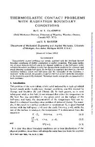
• • N N 4 3 14 18 Figure 1: Lattice configuration σ with weight Wσ = w1 w2 a1 a2 β β12 β2 . Closed bulk loops are not allowed for critical dense polymers with β = 0.
also contains the derivation of the exact finite-size spectra by using empirical physical combinatorics, an Euler-Maclaurin formula and finitized characters. The conformal data is summarized in Section 7 where we relate critical dense polymers with Robin boundary conditions to Z4 fermions. Using results obtained in Appendix C, we also give the fusion rules between Robin modules and the generators of the Kac fusion algebra. Section 8 contains a concluding discussion.
2 2.1
Lattice loop model Statistical lattice model on a strip
We consider a square lattice model of densely packed, non-oriented and non-intersecting loops defined on a rectangular strip of width N and even height M . In a given lattice configuration, a single bulk face contains a pair of loop segments linking the edges pairwise as or
(2.1)
As indicated in the configuration to the left in Figure 1, the left boundary is closed off with half-arcs linking adjacent faces pairwise, while loops can terminate at the right boundary or reflect back into the bulk via half-arcs linking adjacent faces at heights 2j − 1 and 2j, j ∈ N. We distinguish between bulk and boundary loops. First, loops not terminating at the boundary are assigned the bulk loop fugacity β. Second, loops terminating at the right boundary are classified according to whether the lower attachment point is located at an odd or even height. The corresponding boundary loop fugacity is denoted by β1 or β2 , respectively. It is convenient to introduce boundary triangles to describe the possible boundary conditions on the right of the strip. A boundary triangle thus comes with one of the two possible configurations and
(2.2)
where the horizontal line segments indicate that the corresponding loop segments terminate at the boundary. We refer to the boundary conditions in (2.2) as Neumann and Dirichlet boundary conditions, 5
respectively. The configuration on the right in Figure 1 is equivalent to the configuration on the left, and the two types of boundary loops are assigned fugacities as indicated here even odd
.. .
β1 :
.. .
β2 :
(2.3) even
odd
To obtain a statistical model, local Boltzmann weights are assigned to the bulk faces and boundary triangles. The weights w1 and w2 are thus assigned to the bulk faces and , respectively, while the weights a1 and a2 are assigned to the boundary triangles and , respectively. Viewing the loop fugacities as non-local Boltzmann weights, the weight of a lattice configuration σ is thus given by 1 m2 ℓ ℓ1 ℓ2 Wσ = w1n1 w2n2 am 1 a2 β β1 β2
(2.4)
where n1 , n2 , m1 and m2 indicate the numbers of the various faces and triangles in σ, while ℓ, ℓ1 and ℓ2 indicate the numbers of loops. For example, the weight of the configuration in Figure 1 is given by Wσ = w118 w214 a1 a32 β 4 β12 β2 As usual, the partition function is obtained by summing over all possible lattice configurations X Z= Wσ
(2.5)
(2.6)
σ
2.2
Face operators and local relations
To obtain a Yang-Baxter integrable lattice model, we parameterise the bulk loop fugacity as β = 2 cos λ,
0 0, we now impose that boundary links likewise drop down in the sense that if the rightmost node on the upper edge is linked to the boundary, then so is the rightmost node on the lower edge. In the decomposition • 3 3
−u−ξ0
2
u−ξ1
u
= s0 (2u)Γ(ξ + λ)
3 2
• − [Γ(u) + β2 s0 (2u)]s0 (ξ + u)s2 (ξ − u) 1
• • •
3 2
1
+ s0 (2u)s1 (ξ + u)s2 (ξ − u)
•
2 1
(3.24)
1
we thus require that the first coefficient vanishes for all u, that is Γ(ξ + λ) = 0
(3.25)
For w > 0, this imposes a relation between the constant γ and the boundary parameter ξ, γ = β1 [s0 (ξ + λ)]2 − β2 [s0 (ξ + λ2 )]2 so that and hence
� Γ(u) = s1 (ξ − u) β1 s1 (ξ + u) − β2 s0 (ξ + u) � Γ(0) = s1 (ξ) β1 s1 (ξ) − β2 s0 (ξ)
(3.26) (3.27) (3.28)
Combined with the disallowance of half-arcs formed between the w nodes, this is sufficient to ensure that the rule, disallowing boundary links emanating from the w nodes on the lower edge, propagates up through the seam and is thus applicable along the upper edge as well. This is crucial for the construction of the Robin modules in Section 5.2. The combined projection rule that half-arcs between boundary nodes and boundary links emanating from boundary nodes are disallowed can be implemented by the introduction of boundary Wenzl-Jones projectors [58, 59]. We will not discuss this here. Instead, we will follow the approach of [2] and incorporate the rule by modifying the boundary seam and restricting the vector space of link states in Section 5.2. In preparation for this, we now turn to the description of the relevant link states.
4 4.1
Link states Link states and standard modules
A boundary link state on N nodes is a planar diagram of non-crossing arc segments. Such a link state consists of d ∈ {0, . . . , N } vertical line segments (called defects) attached to individual nodes, b ∈ {0, . . . , N } arcs (called boundary links) linking individual nodes to the right boundary, and N −d−b 2 half-arcs connecting nodes pairwise. An arc segment thus emanates from every node so a link state is subject to the parity constraint N − d − b ≡ 0 mod 2 (4.1)
11
As the defects can be thought of linking nodes to the point above at infinity, the requirement of planarity prevents arcs from arching over any of the vertical line segments. An example of a boundary link state on N = 10 nodes with d = 2 defects and b = 2 boundary links is given by (10)
∈ V2,2
(4.2)
(N )
We denote by Vd,b the linear span of the set of link states on N nodes with d defects and b boundary links, and note that � � � � N N (N ) (4.3) dim Vd,b = N −d−b − N −d−b−2 2
2
(N )
The link states themselves thus provide a canonical basis for this vector space. Let Vd denote the set of link states for N and d fixed but with b only constrained by (4.1). The number of these link states is given by � � X N (N ) (N ) dim Vd = (4.4) dim Vd,b = ⌊ N 2−d ⌋ b
For given N , the total number of link states is X X (N ) (N ) dim V (N ) = dim Vd,b = dim Vd = 2N d,b
(4.5)
d
Matrix representations of the one-boundary TL algebra T LN (β; β1 , β2 ) are obtained by letting the algebra generators act on the link states. A standard module of T LN (β; β1 , β2 ), in particular, is defined (N ) for every d ∈ {0, . . . , N } and is obtained by letting the algebra act on Vd in a way that preserves the number of defects. To describe this action, let c be a loop representation of a word in T LN (β; β1 , β2 ) (N ) and v ∈ Vd . The product cv is then given by concatenating the respective diagrams placing v atop (10) c. On V2 , this action is illustrated by
= ββ1 β2
= 0 (4.6)
and is readily seen to give rise to a representation of the algebra. The ensuing standard module is thus (N ) of dimension dim Vd as given in (4.4).
4.2
Robin link states
The link states associated with a Robin boundary condition with boundary seam of width w, as (N +w) , and we described in Proposition 3.2, constitute a subset of the set of boundary link states Vd (N,w) denote the linear span of this subset by Vd . To characterise these Robin link states, we refer to the (N +w) as bulk nodes while the (remaining) w rightmost nodes are N leftmost nodes of a link state in Vd (N +w) (N,w) is now defined by requiring that ⊂ Vd called boundary nodes. A link state in Vd (i) no half-arc is formed between a pair of boundary nodes, (ii) no boundary link emanates from a boundary node. 12
This implies that every boundary node must be a defect or linked to a bulk node. Examples of vector spaces of Robin link states are (3,1)
= span
(3,2)
= span
V1
V1
(4,2)
V0
= span
n
n
n
o ,
o
, ,
(4.7)
,
and the number of these link states is given by � (N,w) dim Vd = � N −d �
,
N � � + (−1)N −d−w w2
2
�
o
(4.8)
For vanishing seam width w = 0, this number correctly reduces to (4.4). Let V (N,w) denote the space of Robin link states with an arbitrary number of defects. The number of these link states is given by dim V (N,w) =
N +w X
(N,w)
= 2N
dim Vd
(4.9)
d=0
and is independent of w.
5 5.1
Transfer matrices Double row transfer tangles
Focusing on scenarios with Neumann boundary conditions on the left but Robin boundary conditions on the right of the strip lattice, as described in Section 2.1, we define the double row transfer tangle λ−u λ−u
D(u) := u
u
|
...
λ−u
...
u
u,ξ
{z
(5.1)
}
N
It is noted that this is an (N +w)-tangle and that the dependence on N , λ, w and ξ has been suppressed. With multiplication given by vertical concatenation of diagrams, and following [60], it follows from the local inversion relation (2.13) and the bulk and boundary Yang-Baxter equations (2.11) and (3.1) that the transfer tangles form a commuting family [D(u), D(v)] = 0,
u, v ∈ C
(5.2)
Using (2.13), (3.10) and (3.22), it also follows that they are crossing symmetric D(λ − u) = D(u)
13
(5.3)
Acting on link states with an auxiliary half-arc between the nodes in positions −1 and 0, transfer matrix representations follow from ‘opening up’ the corresponding transfer tangle as
u u
..
. u
D(u) =
u,ξ
(5.4)
u
.
..
u u
j = −1
0
...
1
N
As an element of T LN +w+2 (β; β1 , β2 ), this is given by (w)
D(u) = e−1 X0 (u)X1 (u) . . . XN −1 (u) KN (u, ξ) XN −1 (u)XN −2 (u) . . . X0 (u)
(5.5)
where the labelling of the nodes starts at j = −1, and where (w)
...
KN (u, ξ) :=
u,ξ
(5.6)
To obtain concrete matrix representations of the transfer tangle, we need to specify the appropriate vector space of link states and the action thereupon by the transfer tangle. As discussed in [2] and in Section 5.2 below, this may affect the description of the tangle itself. Following (5.4), we can also open up the boundary component as
u+ξw u+ξw−1
..
. u+ξ1
u,ξ
=
u u−ξ1
j =
N
.
..
u−ξw−1 u−ξw
j =
N
N+1
14
...
N+w
(5.7)
As an element of T LN +w (β; β1 , β2 ) (or T LN +w+2 (β; β1 , β2 ) if the two auxiliary nodes are included), this is written as � � (w) KN (u, ξ) = XN (u − ξw )XN +1 (u − ξw−1 ) . . . XN +w−1 (u − ξ1 ) Γ(u)I + s0 (2u)fN +w XN +w−1 (u + ξ1 )XN +w−2 (u + ξ2 ) . . . XN (u + ξw )
(5.8)
(N,w)
and when viewed as acting on Vd
, it reduces to
(w)
(w)
(w)
(w)
KN (u, ξ) ≃ α0 I + α1 eN + α2 eN eN +1 + . . . + α(w) w eN eN +1 . . . eN +w−1 (w)
+ αw+1 eN eN +1 . . . eN +w−1 fN +w
(5.9) (N,w)
The fact that the two sides only agree when their actions are restricted to Vd of the similarity sign ≃ instead of an equality sign.
5.2
is reflected in the use
Robin representations
Due to the drop-down properties discussed in Section 3.3, the restriction to the Robin link states (N +2,w) (N,w) if we work with (5.4)) yields well defined representations of the transfer (or Vd spanning Vd tangle (5.1). That is, the drop-down properties ensure that (N,w)
ρd
� � (N,w) � (N,w) D(v) D(u) ρd D(u)D(v) = ρd
(5.10)
(N,w)
(D(u)) is obtained by requiring that the number of where the particular Robin representation ρd defects d is preserved in the same way as in the definition of the standard modules in Section 4.1. More general representations can of course be constructed, but focus here will be on the Robin representations. In the following, we will thus restrict our considerations to the situation where D(u) is meant to (N,w) (w) act on Vd for some d. In a planar decomposition of KN (u, ξ), we may therefore ignore connectivity diagrams containing half-arcs between the w boundary nodes on the lower edge as well as boundary links emanating from these nodes. In the spirit of [2], we thus have the decomposition
u,ξ
(w)
(w)
≃ α0
+ α1 |
(w)
{z
}
w
|
(w)
{z
}
w−1
+ · · · + αk
+ α2
|
{z
w−2
}
+ α(w) w
+ ··· |
(w)
{z k
}
| {z } w−k
•
+ αw+1 |
{z w
}
• |
where the decomposition coefficients are functions of u and ξ. 15
{z w
}
(5.11)
Proposition 5.1 The decomposition coefficients in (5.11) are given by (w)
= Γ(u)η (w) (u, ξ)
(w)
=
α0
αk
(w)
αw+1 =
(−1)k s0 (2u)η (w) (u, ξ) � Uw−k s0 (u + ξ)sw+1 (ξ − u)
β� 2 Γ(u)
(−1)w s0 (2u)s1 (ξ − u)η (w) (u, ξ) sw+1 (ξ − u)
� − β1 sw−k+1 (u + ξ)s1 (ξ − u) ,
k = 1, 2, . . . , w (5.12)
where Un (x) is the n-th Chebyshev polynomial of the second kind and η
(w)
(u, ξ) :=
w Y
s−1 (u + ξj )s−1 (u − ξj )
(5.13)
j=1
Proof: For w = 0, the coefficients reduce to (0)
(0)
α0 = Γ(u),
α1 = s0 (2u)
(5.14)
in accordance with the decomposition of the twist boundary condition (3.3). For w = 1, we have −u−ξ0
u
� � + s0 (2u) Γ(u) + β1 s0 (u + ξ1 )s0 (u − ξ1 )
= η (1) (u, ξ) Γ(u)
u−ξ1
• − s0 (2u)s0 (u + ξ)s0 (u − ξ1 ) � + s0 (2u) η (1) (u, ξ) (1)
≃ α0
•
• •
− s1 (u + ξ)s0 (u − ξ2 )
(1)
+ α1
(1)
+ α2
•� •
• (5.15) •
thus reproducing (5.12). The proof is now completed by induction in w. Introducing the shorthand notation v = −u − ξw−1 , we observe that v
+ s0 (2u)
= s−1 (u + ξw )s−1 (u − ξw ) u−ξw
v
− s−1 (u + ξw )s0 (u − ξw )
≃ s0 (u + ξw )s0 (u − ξw ) u−ξw
v
≃ −s−1 (u + ξw )s0 (u − ξw ) u−ξw
16
(5.16)
and •
•
−u−ξ1
•
u−ξ2
(5.17)
≃ −s0 (u + ξ1 )s0 (u − ξ2 )
•
where the relation (5.17) is relevant for w = 2 only. For general w ≥ 2, we then deduce that (w)
= s0 (u + ξw−1 )s0 (u − ξw+1 )α0
(w)
= s0 (2u)α0
(w)
= −s0 (u + ξw−1 )s0 (u − ξw )αk−1 ,
α0
α1
αk
(w−1)
(w−1)
(w−1)
+ s0 (u + ξw )s0 (u − ξw )α1 (w−1)
Using that s0 (u + ξ) + Uw−2
β� 2 s0 (u
k = 2, . . . , w + 1
+ ξw ) = Uw−1
β� 2 s0 (u
(5.18)
+ ξw−1 )
(5.19)
the recursion relations (5.18) are seen to be satisfied by (5.12). This completes the induction step and hence the proof. �
Renormalised transfer tangles for β 6= 0
5.3
Here we assume β 6= 0. The case β = 0 corresponds to critical dense polymers LM(1, 2) and is treated separately in Section 6. It is convenient to introduce the renormalised transfer tangle d(u) :=
1 D(u), η(u)
η(u) :=
β Γ(0)sw (u + ξ)s0 (ξ)η (w) (u, ξ) s0 (u + ξ)sw (ξ)
(5.20)
noting that the normalisation function reduces to η(u) = β Γ(0) for w = 0. Renormalising the decomposition coefficients (5.12) accordingly (w) α (w) α ˆ k := k (5.21) η(u) yields (w)
α ˆ0
(w)
α ˆk
Γ(u)s0 (u + ξ)sw (ξ) β Γ(0)sw (u + ξ)s0 (ξ) � � � (−1)k s0 (2u)sw (ξ) Uw−k β2 Γ(u) − β1 sw−k+1 (u + ξ)s1 (ξ − u) = , β Γ(0)sw+1 (ξ − u)sw (u + ξ)s0 (ξ) =
(w)
α ˆ w+1 =
k = 1, . . . , w
(−1)w s0 (2u)s1 (ξ − u)s0 (u + ξ)sw (ξ) β Γ(0)sw+1 (ξ − u)sw (u + ξ)s0 (ξ)
(5.22)
This renormalisation ensures that lim d(u) ≃ I
(5.23)
u→0
since lim d(u) ≃
u→0
1 lim β u→0
λ−u λ−u u
|
u
. . . λ−u
... {z N
u
}|
... ... {z w
= } 17
1 β |
...
...
... {z
... {z
N
}|
w
(5.24) }
where the first relation is a consequence of (w)
lim α ˆ0
u→0
=
1 , β
(w)
lim α ˆk
u→0
= 0,
k = 1, . . . , w + 1
(5.25)
Due to η(λ − u) = η(u)
(5.26)
the renormalisation also preserves the crossing symmetry d(λ − u) = d(u)
(5.27)
It is noted that the normalisation (5.20) is not uniquely determined by requiring the renormalised transfer tangle to have the properties (5.23) and (5.27).
5.4
Hamiltonians for β 6= 0
The Hamiltonian is obtained by expanding the renormalised double row transfer tangle as d(u) = I −
2u (H + hI) + O(u2 ) sin λ
(5.28)
where h measures a convenient shift in the groundstate energy. Recalling the Robin representation (N,w) (N,w) (H) of H is introduced as (D(u)) discussed in Section 5.2, the matrix representation ρd ρd (N,w)
ρd
(H) = −
� sin λ ∂ (N,w) d(u) − hI ρd 2 ∂u u=0
(5.29)
where I is the identity matrix of the appropriate size. We now assume β 6= 0. The case β = 0 corresponds to critical dense polymers LM(1, 2) and is treated separately in Section 6. For β 6= 0, we set � Uw−1 β2 Nβ 1 β2 h= − + − (5.30) 2 β 2 Γ(0) 2s0 (ξ)sw (ξ) and note that the last contribution vanishes for w = 0 since U−1 (x) ≡ 0. (N,w)
Proposition 5.2 As an element of T LN +w (β; β1 , β2 ) designed to act on Vd tonian for β 6= 0 is given by H≃−
N −1 X j=1
ej −
w X k=1
� (−1)k Uw−k s0 (ξ)sw+1 (ξ)
−(−1)w
β� 2
−
β1 s1 (ξ)sw−k+1 (ξ) � eN eN +1 . . . eN +k−1 Γ(0)
s1 (ξ) eN eN +1 . . . eN +w−1 fN +w sw+1 (ξ)Γ(0)
18
for any d, the Hamil-
(5.31)
Proof: To keep the presentation simple, we first focus on the situation where w = 0. In this case, we have ! λ−u λ−u λ−u λ−u . . . λ−u λ−u λ−u λ−u λ−u . . . λ−u • 1 + s0 (2u) Γ(u) d(u) = η(u) u u u u ... u u u u u ... u • [s1 (−u)]2N = η(u)
...
Γ(u)
+ s0 (2u)
...
...
s0 (u)[s1 (−u)]2N −1 Γ(u) η(u)
+
... ... ...
+
... ...
+
... ...
+... +
...
...
! • •
...
+
...
+
...
... ...
+
(5.32)
... ...
+
... ...
+
... ...
+
...
!
+ O(u2 )
and using the explicit power series expansions [s1 (−u)]n = 1 − n(cot λ)u + O(u2 ),
s0 (nu) =
n u + O(u2 ), sin λ
Γ(u) = Γ(0) −
β2 u + O(u2 ) sin λ (5.33)
we identify the Hamiltonian (5.31) H=−
N −1 X
ej −
j=1
1 fN , Γ(0)
w=0
(5.34)
The generalisation to w > 0 is straightforward and follows from β� 1 u � Uw−1 2 β2 � (w) α ˆ0 = + + O(u2 ) − β sin 2λ s0 (ξ)sw (ξ) Γ(0) (w)
α ˆk
(w)
=
α ˆ w+1 =
� 2u (−1)k Uw−k sin 2λ s0 (ξ)sw+1 (ξ)
β� 2
2u (−1)w s1 (ξ) + O(u2 ) sin 2λ Γ(0)sw+1 (ξ)
−
β1 s1 (ξ)sw−k+1 (ξ) � + O(u2 ), Γ(0)
k = 1, . . . , w (5.35) �
19
6
Critical dense polymers
Critical dense polymers is described by the logarithmic minimal model LM(1, 2). Since λ = case, the bulk loop fugacity is zero, β=0
π 2
in this (6.1)
thus disallowing closed loops in the bulk. In Section 6.1, we will keep the boundary loop fugacities β1 and β2 arbitrary, but set them equal to 1 in Section 6.2 and subsequent sections. For those special values, one can simply ignore all boundary loops as they merely contribute factors of 1.
6.1
Hamiltonian limit
For β = 0, we introduce the renormalised transfer tangle d(u) :=
1 D(u), η(u)
η(u) :=
Γ(0)s0 (2u)sw (u + ξ)s0 (ξ)η (w) (u, ξ) s0 (u + ξ)sw (ξ)
(6.2)
noting that the normalisation function reduces to η(u) = Γ(0)s0 (2u) for w = 0. As for β 6= 0 in Section 5.3, this normalisation ensures that lim d(u) ≃ I,
d(λ − u) = d(u)
u→0
(6.3)
The Hamiltonian is obtained as in (5.28), but with h in (5.30) replaced by h=
β2 (−1)w − 1 + 2 Γ(0) 2s0 (2ξ)
(6.4)
(N,w)
Proposition 6.1 As an element of T LN +w (0; β1 , β2 ) designed to act on Vd tonian is given by H ≃ −
N −1 X j=1
for any d, the Hamil-
� � w X (−1)k s1 (ξ) (w − k + 1)π (w − k + 1)π + β2 sin ej + β1 cos eN eN +1 . . . eN +k−1 Γ(0)sw+1 (ξ) 2 2 k=1
−
(−1)w s1 (ξ) eN eN +1 . . . eN +w−1 fN +w Γ(0)sw+1 (ξ)
(6.5)
Proof: Because β = 0, we need to expand D(u) to second order in u. Using techniques similar to the ones employed in the proof of Proposition 5.2, we first expand the bulk part of the transfer tangle λ−u λ−u u
u
... ...
= 2u u
u
...
u
...
+ 4u2
1 + 2
...
λ−u λ−u λ−u
... ... ...
... + ... +
1 + 2
20
... ... ...
!
+ O(u3 )
(6.6)
Next, we glue these diagrams together with the diagrams in the decomposition (5.11) to form D(u) in (5.1). This is illustrated here by gluing together the last diagram in (6.6) with the diagram whose (w) coefficient in (5.11) is α1 ,
|
...
...
...
...
{z
}
N
|
{z w
= eN eN −1
(6.7)
}
As it turns out, this composite diagram does not contribute to the Hamiltonian. To see this and determine the ones that do contribute, we must combine the power series expansion of D(u) with that (w) of the normalisation function η(u). Thus, writing the expansion of the u-dependent coefficients αk as (w)
αk
(w)
we observe that
αk,0 , αk,1 ∈ R,
(w)
αk,0 = 0, while writing
(w)
(w)
(w)
= αk,0 + αk,1 u + O(u2 ),
k = 0, . . . , w + 1
k = 1, . . . , w + 1
η−1 1 = + η0 + O(u), η(u) u
we note that η−1 =
(6.8) (6.9)
η−1 , η0 ∈ R
(6.10)
1
(6.11)
(w)
2α0,0
This last relation must be satisfied to ensure the limit in (6.3) and is readily verified. Combining these results yields (w)
h=
α0,1
(w) − (w) − η0 α0,0 , 2α0,0
H≃−
N −1 X
ej −
j=1
(w) w X αk,1
(w)
2α0,0
k=1
(w)
eN . . . eN +k−1 −
αw+1,1 (w)
2α0,0
eN . . . eN +w−1 fN +w
(6.12) where we have identified h as the coefficient to −2uI in the expansion of d(u). It is noted that this (w) expression for H is independent of η0 . With the concrete expressions for αk , k = 0, . . . , w + 1, in � (5.12) and η(u) in (6.2), we finally obtain (6.4) and (6.5). For w = 0, (6.5) becomes the equality H=−
N −1 X
ej −
j=1
6.2
1 fN Γ(0)
(6.13)
Special parameter values
From here onwards, we fix the boundary loop fugacities to the values β1 = β2 = 1
(6.14)
allowing us to ignore all boundary loops. For w > 0, we furthermore restrict our considerations to the special value λ π ξ=− =− (6.15) 2 4 21
in which case (3.26) implies that γ = 21 . Extending this to w = 0, we thus have Γ(u) = cos u (cos u − sin u),
Γ(0) = 1
(6.16)
for all seam widths w ∈ N0 . Since η (w) (u, − π4 ) = the renormalised transfer tangle is given by
�1
�w cos 2u 2
� 2w cos u − sin u � D(u), d(u) = sin 2u [cos 2u]w cos u − (−1)w sin u
(6.17)
w ∈ N0
(6.18)
The corresponding shift in groundstate energy is
h = 1 − 12 (−1)w ,
w ∈ N0
(6.19)
(N,w)
for any d, the Hamiltonian Corollary 6.2 As an element of T LN +w (0; 1, 1) designed to act on Vd is given by w N X X k+1 (−1)⌊ 2 ⌋+(k−1)w eN eN +1 . . . eN +k ej + H≃− (6.20) j=1
k=1
where eN +w ≡ fN +w . For w = 0, this becomes the equality H=−
N −1 X
ej − fN
(6.21)
j=1
(N,w)
(H) (5.29) of H given in (6.20) can be computed by acting with The matrix representation ρd (3,1) (3,2) (4,2) (N,w) . With bases of V1 , V1 and V0 as indicated in (4.7), we thus find H on Vd (3,1)
ρ1 (H) = −(0) − (0) − (0) + (1) = (1) (6.22) 1 0 1 0 0 0 1 0 1 0 0 0 0 0 0 0 0 0 (3,2) ρ1 (H) = − 1 0 1 − 0 0 0 − 0 0 1 − 0 1 0 + 0 0 0 = − 1 1 2 0 1 0 0 0 0 0 0 0 0 0 0 0 1 0 0 0 0 (6.23) and 0 1 1 0 0 0 0 0 0 0 0 0 0 0 0 0 0 0 0 0 0 0 0 0 0 0 0 0 0 0 0 0 (4,2) ρ0 (H) = − 0 0 0 0 − 1 0 0 1 − 0 0 0 0 − 0 0 0 1 0 0 0 0 0 0 0 0 0 0 1 0 0 0 0 0 1 0 0 1 0 0 0 0 1 1 1 1 0 1 0 0 0 0 0 1 0 1 0 −1 − (6.24) 0 0 1 0 + 0 0 0 0 = − 1 0 1 2 0 0 0 0 0 0 0 0 0 0 1 0 22
6.3
Inversion identity
With the parameters β1 , β2 and ξ fixed as in (6.14) and (6.15), the renormalised transfer tangle d(u) satisfies the inversion identity given in Proposition 6.3 below. This is generalised to all β1 , β2 and ξ in Appendix B where we also present a proof of the inversion identity in the general case. Proposition 6.3 As elements of T LN +w (0; 1, 1), the renormalised transfer tangles with ξ = − π4 satisfy the inversion identity cos4N +2 u − sin4N +2 u d(u)d(u + π2 ) = I (6.25) cos2 u − sin2 u It is noted that the exact same inversion identity holds for the corresponding algebra elements designed (N,w) , as described in Section 5.2. This is thanks to the drop-down properties of Section 3.3. to act on Vd It is stressed that the inversion identity is independent of the width w of the boundary seam.
6.4
Exact solution for eigenvalues (N,w)
It follows from Proposition 6.3 and the properties (6.3) that the eigenvalues Λn (u) of ρd of the form N N � � Y 1 Y (n) (n) 1 + ǫj sin tj sin 2u , ǫj sin 2u + cosec tj = Λn (u) = N 2
n = 0, 1, 2, . . .
(d(u)) are
(6.26)
j=1
j=1
where (n)
ǫj
= ±1,
tj =
(j − 12 )π , 2N + 1
j = 1, . . . , N
(6.27)
(n)
Selection rules specifying the signs ǫj are found empirically and discussed in the following. From the crossing symmetry and periodicity, the zeros uj of an eigenvalue Λn (u) occur in complex conjugate pairs in the complex u-plane and appear with a periodicity π in the real part of u. For these reasons, we restrict our attention to the fundamental strip in the lower-half plane −
π 3π < Re u ≤ , 4 4
Im u ≤ 0
(6.28)
From (6.26), the zeros uj inside or on the boundary of the fundamental strip are located at uj = (2 + ǫj )
tj i π + ln tan , 4 2 2
ǫj = ±1
(6.29)
Thus, the ordinates of the locations of these zeros are yj =
1 2
ln tan 12 tj ,
j = 1, 2, . . . , N
(6.30)
If ǫj = −1, there is a single zero or “1-string” inside the fundamental strip at u = π4 + iyj . If ǫj = +1, there are zeros at u = − π4 + iyj and u = 3π 4 + iyj on the boundary of the strip, and we refer to them as forming a “2-string”. A typical pattern of zeros for N = 5 is shown in Figure 2.
23
−y1
−y2 −y3 −y4 −y5 − π4
π 4
y5 y4
π 2
3π 4
y3 y2
y1
Figure 2: A typical pattern of zeros in the complex u-plane for N = 5. The pattern of zeros is symmetric under complex conjugation of u. The ordinates of the locations of the zeros uj in the lower-half plane are yj = 12 log tan (2j−1)π 4N +2 , j = 1, 2, . . . , N . At each position j, there is either a 1-string with Re uj = π/4 or a 2-string with Re uj = −π/4, 3π/4. Each such pattern is encoded by the subset En of j indices for which ǫj = −1. For each j ∈ En , the eigenvalue Λn (u) has a 1-string in the fundamental strip with ordinate y = yj with excitation energy Ej = 12 (j − 21 ). For the eigenvalue shown, En = {3, 5} and E(En ) = E3 + E5 = 54 + 94 = 72 .
6.5
Finite-size corrections (N,w)
The eigenvalues Λn (u) of the transfer matrix ρd Λn (u) =
N Y
(d(u)) are of the form
(n)
(1 + ǫj sin tj sin 2u),
n = 0, 1, 2, . . .
(6.31)
j=1
where tj is defined in (6.27). Let En be the subset of j indices for which ǫj = −1. A particular (n) eigenvalue Λn (u) is determined by the pattern En of values for ǫj . In principle, there are 2N different patterns giving 2N possible eigenvalues but only a subset of these occur as eigenvalues of the transfer matrix for a given Robin boundary condition. The set of allowed patterns En that actually occur thus depends on d and w and its specification is encoded in selection rules. Conformal invariance dictates that, for large N , the transfer matrix eigenenergies take the form En (u) = − ln Λn (u) = 2N fbulk (u)+fbdy (u)+
� 2π sin 2u 1 � c , − +∆+k +O N 24 N2
n = 0, 1, 2, . . . (6.32)
where fbulk (u) is the bulk free energy per face, fbdy (u) the boundary free energy, c is the central charge and ∆ is a conformal dimension determined by the boundary condition. The non-negative integer k is associated with descendants in the tower of eigenenergies and depends on the transfer matrix eigenvalue label n with k = 0 for n = 0. 24
Let us introduce the function F (t) = ln(1 + sin t sin 2u)
(6.33)
where for simplicity the u dependence has been suppressed. As a partial evaluation of the energies (6.32), we find ln
N Y
j=1
� (n) 1 + ǫj sin tj sin 2u =
1 2
2N +1 X
F (tj ) − 21 F ( π2 ) −
j=1
1 � 2π sin 2u X Ej + O N N2
(6.34)
j∈En
where F ( π2 ) = ln(1 + sin 2u) and the conformal energies of elementary finite excitations are Ej = 21 (j − 21 )
(6.35)
This formula is valid for finite excitations for which the subset En remains finite as N → ∞. The finite-size corrections in (6.32) are determined by applying an appropriate Euler-Maclaurin formula. The midpoint Euler-Maclaurin formula is m X
F a + (j −
j=1
�
1 2 )h
1 = h
Z
b
F (t) dt −
a
� h ′ [F (b) − F ′ (a)] + O h2 24
(6.36)
where a = 0, b = π, m = 2N + 1 and h = (b − a)/m = π/(2N + 1). This formula is valid since F (t) and its first two derivatives are continuous on the closed interval [a, b] = [0, π/2]. Applying this formula, we find X � 1 � 1 2π sin 2u Ej + O (6.37) + − En (u) = 2N fbulk (u) + fbdy (u) + N 96 N2 j∈En
In these expressions, the bulk free energy per face is given by 1 fbulk (u) = − π
Z
π/2
ln(1 + sin t sin 2u)dt
(6.38)
0
whereas the boundary free energy is given by fbdy (u) = fbulk (u) + 21 F ( π2 )
(6.39)
We conclude that −
X c 1 Ej , +∆=− + 24 96
3 + ∆ = − 32
X
1 2 (j
− 21 )
(6.40)
j∈En
j∈En
where c = −2
(6.41)
From Section 6.6, the minimum energy for a twist boundary condition (w = 0) with a fixed number of defects d is 81 d(d + 1). It follows that for these groundstate patterns En , as in Figure 4, 3 3 5 21 45 77 ∆0,d+ 1 = − 32 + 18 d(d + 1) = − 32 , 32 , 32 , 32 , 32 , . . . , 2
d = 0, 1, 2, 3, 4, . . .
(6.42)
The link between the lattice model and the CFT characters is governed by the modular nome q = e−2πτ ,
τ = δ sin ϑ 25
(6.43)
where δ = M/N is the aspect ratio and ϑ = 2u is the anisotropy angle [61] related to the geometry of the lattice. For a given boundary condition, the excitations form a conformal tower, indexed by k in (6.32), with integer spacings above the lowest energy state given by the corresponding conformal 3 , occurs when ǫj = +1 for all j. Consider weight ∆. The lowest groundstate energy, with ∆ = − 32 an elementary finite excitation where only one ǫj = −1. This corresponds to a single 1-string in the fundamental strip. Taking the ratio of (6.31) with precisely one ǫj = −1 to (6.31) with all ǫj = +1, and taking the limit M, N → ∞ with a fixed aspect ratio δ = M/N gives lim
M,N →∞
�
1 − sin (2j−1)π 4N +2 sin 2u 1 + sin
(2j−1)π 4N +2
sin 2u
�M
= exp[−(j − 21 )π δ sin 2u] = q Ej
where the conformal energies of elementary finite excitations are given by (6.35). It follows that the conformal partition functions take the form X c Z(q) = q − 24 +∆ q E(En )
(6.44)
(6.45)
allowed En
where the total conformal energy of an allowed pattern En with n = 0, 1, 2, . . . is X Ej E(En ) =
(6.46)
j∈En
6.6
Physical combinatorics and finitized characters
Following the description of the Z4 sectors of critical dense polymers on the cylinder [49], the patterns of zeros of Λn (u) are conveniently encoded by single column diagrams as shown in Figure 3. The single column corresponds to the 1-strings in the lower-half u-plane. Positions j = 1, 2, . . . , N occupied by a 1-string are indicated by a solid red or blue circle for j odd or even, respectively. The unoccupied positions are indicated by an open circle. The number of 1-strings mj = 0, 1 plus the number of 2-strings nj = 0, 1 at any given position is one mj + nj = 1,
j = 1, 2, . . . , N
(6.47)
Each single column diagram {m1 , m2 , . . . , mN } is associated with a monomial qE = q
PN
j=1
mj Ej
(6.48)
The energy E of a finite excitation can be incremented by one unit either by inserting a pair of 1-strings at positions j = 1 and j = 2 or by incrementing the position j of a single 1-string by 2 units. It follows that the excess ⌊n/2⌋
σ := meven − modd =
X k=1
⌊(n+1)/2⌋
m2k −
X
m2k−1
(6.49)
k=1
given by the number of (blue) 1-strings at even positions j minus the number of (red) 1-strings at odd positions j, is a quantum number. The single column diagrams with a given quantum number σ are generated combinatorially by starting with the minimum energy configuration of 1-strings. The minimum energy configurations, for given σ, are shown in Figure 4. The energy of such a minimum energy configuration is (6.50) Emin = 12 σ(σ + 12 ) 26
j=N j = N −1
.. .
1
j=3
3
5
9
9
q 4+4+4+4 = q 2
↔
j=2 j=1
Figure 3: The pattern of zeros of Λn (u) is encoded by a single column diagram. The column corresponds to the 1-strings in the lower-half u-plane. Positions occupied by a 1-string are indicated by a solid red or blue circle for j odd or even, respectively. Unoccupied positions are indicated by an open circle. The 1-string energies are given by Ej = 12 (j − 21 ). For the eigenvalue depicted, N = 6, σ = −2, E = 92 9 and the associated monomial is q E = q 2 .
j=7 j=6 j=5 j=4 j=3 j=2 j=1
σ
3
2
1
0
−1
−2
−3
−4
Figure 4: Minimal energy configurations of the single column diagrams. The minimal energy is Emin = 1 1 2 σ(σ + 2 ). The quantum number σ is given by the excess of blue (even j) over red (odd j) 1-strings. At each empty position j, there is a 2-string.
27
j=7 j=6 j=5 j=4 j=3 j=2 j=1
�7�
5 q
=
1 + q + 2q 2 + 2q 3 + 3q 4 + 3q 5 + 3q 6 + 2q 7 + 2q 8 + q 9 + q 10
Figure 5: For n = 7, σ = −2, m = ⌊n/2⌋ − shows combinatorial enumeration by � nσ� = 5,�7the � figure P P the −3/2 j mj Ej . The excess of blue (even j) single column diagrams of the q-binomial m = = q q 5 q q over red (odd j) 1-strings is given by the quantum number σ = −2. The excitation energy of a 1-string at position j is Ej = 21 (j− 12 ). The lowest energy configuration has energy Emin = 41 + 45 = 32 = 21 σ(σ+ 21 ). At each empty position j, there is a 2-string. Excitation increments (of energy 1) are generated by either inserting two 1-strings� at� positions � n �j = 1 and j = 2 or promoting a 1-string at position j to n position j + 2. Notice that m q = n−m q as q-polynomials, but they have different combinatorial interpretations because they have different quantum numbers σ. For modest system sizes N , extensive numerics were carried out in Mathematica [62] to obtain (N,w) (d(u)) for the various sectors with d the finite-size eigenvalue spectra of the transfer matrices ρd defects and a boundary seam of width w. The exact conformal eigenenergies are read off from the patterns of 1-strings and 2-strings in the complex u-plane by summing the energies Ej = 12 (j − 12 ) of the elementary 1-string excitations. The quantum number σ is read off from the excess of even (blue) 1-strings over odd (red) 1-strings. From this analysis it is found that, in a sector with given N and σ, the conformal spectrum or finitized partition function is described by a single normalized q-binomial of the form � � � � X P 1 3 1 c N (N ) + 32 σ(σ+ 12 ) N σ(σ+ 12 ) 24 2 2 χ = q j mj Ej , σ = ⌊ N2 ⌋ − m (6.51) =q q σ (q) = q m q ⌊ N2 ⌋ − σ q σ-single columns
The sum is over all single column diagrams, as in Figure 5, associated with the fixed quantum number σ. In particular, this analysis yields expressions, in terms of the quantum numbers d and w, for the lowest energy eigenvalues in each sector. Equating these expressions for the lowest energies to (6.50) 28
gives the quadratic equation � 1 8
(d +
1 2
− 2r)2 −
1 4
�
= 21 σ(σ + 12 ) = ∆r,s− 1 + 2
3 32
(6.52)
where we have implicitly imposed selection rules according to the empirical identifications ( N even (−1)d+w ⌈ w2 ⌉, s = d + 1, r= w d+w −(−1) ⌈ 2 ⌉, N odd
(6.53)
This is the usual identification between s and d [1], but we have allowed r ∈ Z to take negative values. Solving the quadratic equation (6.52) gives a unique result for the integer σ ( ( d 1 2(r + σ), d even 2 − r = − 2 (2r − s + 1), d even (s odd) (6.54) d = σ= 1 2(r − σ) − 1, d odd = (2r − s), d odd (s even) r − d+1 2 2 On a finite lattice, the ranges of the quantum numbers d and σ are given by −⌊ N 2+1 ⌋ ≤ σ ≤ ⌊ N2 ⌋
0 ≤ d ≤ N + w,
(6.55)
where each allowed value of the quantum number σ occurs exactly once but, depending on N and w > 0, some sectors given by certain disallowed values of d are empty. This occurs precisely when σ = σ(d, w), given by (6.54), is outside of the allowed range (6.55). For the twist boundary condition with r = w = 0, the quantum number σ of the groundstate with d defects simplifies to ( ( d � � 2σ, σ≥0 , d even d d 2 (6.56) , d= σ = (−1) 2 = d+1 −(2σ + 1), σ < 0 − 2 , d odd
Using the q-binomial building blocks (6.51), the empirical selection rules (6.53) and summing over all of the sectors (labelled by σ and weighted by z −σ ) gives the generating function for the finitized conformal partition functions ⌋ ⌊N 2
Z
(N )
(q, z) =
X
z
−σ
) χ(N σ (q)
=q
σ=−⌊ N+1 ⌋ 2
=q
3 c − 32 − 24
k=1
X
q
1 σ(σ+ 12 ) 2
σ=−⌊ N+1 ⌋ 2 ⌊ N+1 ⌋
⌊N ⌋ 2
Y
⌋ ⌊N 2
3 c − 32 − 24
1+q
k− 41 −1
z
2 � Y
k=1
3
1 + q k− 4 z
�
z
−σ
�
N ⌊ N2 ⌋ − σ
�
q
(6.57)
This partition function is independent of d and w and, as discussed in Section 7, coincides with the (N ) corresponding character of Z4 fermion. Varying w acts to shuffle the building blocks χσ (q) among the contributions from different defect numbers. This reshuffling is made manifest by rewriting the partition function as � � N +w c 3 X 1 1 N N−d−w ⌈ w ⌉)2 − 1 ] (−1)N+w ⌈ w ⌉−(−1)d ⌈ d ⌉ 2 4 z 2 2 Z (N ) (q, z) = q − 24 − 32 q 8 [(d+ 2 −2(−1) ⌊ N 2−d ⌋ + (−1)N −d−w ⌈ w2 ⌉ q d=0 (6.58) As already indicated, despite the appearance of w, the partition function is independent of w. We also note that Z (N ) (1, 1) = 2N (6.59) which reflects the counting of Robin link states in (4.9). This is in accord with the empirical observation that each allowed eigenvalue appears exactly once in these partition functions. 29
7 7.1
Conformal field theory Conformal data
In the discussion of the lattice model above, w denotes the width of the boundary seam and d the number of defects. For ξ = − λ2 = − π4 as in (6.15), it was found that, in the continuum scaling limit, the Robin representations give rise to Virasoro Verma characters of conformal weights given by � � r = (−1)N −d−w w2 , s=d+1 (7.1) ∆ = ∆r,s− 1 , 2
where the Kac formula (1.1) for critical dense polymers LM(1, 2) with central charge c = −2 is given by (2r − s)2 − 1 (7.2) ∆r,s = ∆1,2 = r,s 8 The corresponding Kac table for ∆r,s− 1 with r, s ∈ Z is given in Figure 6 where we have included 2 s ∈ −N0 to facilitate the description of the fusion rules in Section 7.5. Here we note that each conformal weight in the Kac table in Figure 6 appears exactly once in either of the two sets � � ∆r, 1 ; r ∈ Z (7.3) ∆0,s− 1 ; s ∈ N , 2
2
corresponding respectively to the shaded central half-column or central row. In the following, we will primarily work with the weights labeled as in the central row where ∆r, 1 = − 2
r(2r − 1) 3 + , 32 4
r∈Z
For Robin boundary conditions where r ∈ Z and s ∈ N, we thus have ∆r− s−1 , 1 , s odd 2 2 ∆r,s− 1 = ∆−σ, 1 = 2 2 ∆ s even −r+ s , 1 ,
(7.4)
(7.5)
2 2
We denote by V (∆) the (highest-weight) Virasoro Verma module of conformal weight ∆, while the corresponding irreducible highest-weight Virasoro module is denoted by V(∆). Two irreducible highest-weight modules of the same conformal weight are isomorphic and can be identified. A Verma module, whose conformal weight is not in the infinitely extended integer Kac table, is irreducible and cannot appear as a proper subquotient of an indecomposable module. A Verma module V (∆r,s− 1 ) 2 with ∆r,s− 1 in Figure 6 is of this type, implying that 2
V (∆r,s− 1 ) = V(∆r,s− 1 ), 2
2
r, s ∈ Z
(7.6)
The Verma modules V (∆r,s− 1 ) and V (∆r′ ,s′ − 1 ) at (integer) positions (r, s) and (r ′ , s′ ) are therefore 2 2 isomorphic when the conformal weights coincide, that is, when |4r − 2s + 1| = |4r ′ − 2s′ + 1|. Explicitly, this occurs if 2r − s = 2r ′ − s′ or 2r − s + 2r ′ − s′ = −1.
7.2
Z4 fermions and Virasoro modules
We consider the spin-1 chiral fermion system η(z) and ξ(z) satisfying the standard operator product expansion 1 (7.7) η(z)ξ(w) = z−w 30
.. .
.. .
.. .
.. .
.. .
.. .
.. .
.. .
.. .
.. .
.. .
..
···
1085 32
837 32
621 32
437 32
285 32
165 32
77 32
21 32
3 − 32
5 32
45 32
···
6
···
957 32
725 32
525 32
357 32
221 32
117 32
45 32
5 32
3 − 32
21 32
77 32
···
5
···
837 32
621 32
437 32
285 32
165 32
77 32
21 32
3 − 32
5 32
45 32
117 32
···
4
···
725 32
525 32
357 32
221 32
117 32
45 32
5 32
3 − 32
21 32
77 32
165 32
···
3
···
621 32
437 32
285 32
165 32
77 32
21 32
3 − 32
5 32
45 32
117 32
221 32
···
2
···
525 32
357 32
221 32
117 32
45 32
5 32
3 − 32
21 32
77 32
165 32
285 32
···
1
···
437 32
285 32
165 32
77 32
21 32
3 − 32
5 32
45 32
117 32
221 32
357 32
···
0
···
357 32
221 32
117 32
45 32
5 32
3 − 32
21 32
77 32
165 32
285 32
437 32
···
−1
···
285 32
165 32
77 32
21 32
3 − 32
5 32
45 32
117 32
221 32
357 32
525 32
···
−2
···
221 32
117 32
45 32
5 32
3 − 32
21 32
77 32
165 32
285 32
437 32
621 32
···
−3
···
165 32
77 32
21 32
3 − 32
5 32
45 32
117 32
221 32
357 32
525 32
725 32
···
−4
···
117 32
45 32
5 32
3 − 32
21 32
77 32
165 32
285 32
437 32
621 32
837 32
···
−5
···
77 32
21 32
3 − 32
5 32
45 32
117 32
221 32
357 32
525 32
725 32
957 32
···
.. .
.. .
.. .
.. .
.. .
.. .
.. .
.. .
.. .
.. .
.. .
..
−5
−4
−3
−2
−1
0
1
2
3
4
5
r
s
..
7
..
.
.
.
.
Figure 6: Kac table of conformal weights ∆r,s− 1 for critical dense polymers LM(1, 2). The structure 2 of the table encodes the sl(2) fusion (7.64) with the fundamental Kac modules (2, 1) and (1, 2). The physical boundary conditions corresponding to w, d ≥ 0 are given by s ≥ 1.
31
The corresponding energy-momentum tensor is given by T (z) = − : η(z)∂ξ(z) : and the modes of T defined by T (z) =
X
(7.8)
z −n−2 Ln
(7.9)
n∈Z
satisfy the Virasoro algebra
[Ln , Lm ] = (n − m)Ln+m +
c n(n2 − 1)δn+m,0 12
(7.10)
with central charge c = −2. Here we are interested in the Z4 sector of the fermions (see a detailed description in [47]), which means that the fields η(z) and ξ(z) satisfy twisted periodicity conditions with respect to adding 2π to the argument α of z = ρeiα , that is πi
η(ρei(α+2π) ) = e− 2 η(ρeiα ),
πi
ξ(ρei(α+2π) ) = e 2 ξ(ρeiα ),
ρ, α ∈ R
(7.11)
The fields η(z) and ξ(z) should thus be considered as living on a Riemann surface with four sheets, not on the complex plane. Under the periodicity conditions (7.11), η(z) and ξ(z) have the following mode decompositions X X z −k−1 ηk , ξ(z) = z −k ξk (7.12) η(z) = k∈Z+ 14
k∈Z− 14
These modes satisfy the anti-commutation rules � � � ηn+ 1 , ηm+ 1 = ξn− 1 , ξm− 1 = 0, ηn+ 1 , ξm− 1 = δn+m,0 , 4
4
4
4
4
4
n, m ∈ Z
(7.13)
With normal ordering defined by
: ηn+ 1 ξm− 1 := 4
4
ηn+ 1 ξm− 1 , 4
n0 , F − := ηk− 3 , ξk− 1 ; k ∈ Z≤0 (7.16) 4
4
4
4
3 i in the Z4 sector is now characterised by the annihilation and eigenvalue condiThe groundstate |− 32 tions 3 3 3 3 i = 0, L0 |− 32 i = − 32 |− 32 i (7.17) F + |− 32
in accordance with (7.15), and the space V4 is generated by the free action of {I} ∪ F − on this groundstate � 3 3 i, F − |− 32 i (7.18) V4 = span |− 32 32
By construction, the space V4 is graded by L0 and thus decomposes into L0 eigenspaces. Another useful grading is with respect to the zero mode of the U (1) current X J(z) = − : η(z)ξ(z) :, J(z) = z −n−1 Jn
(7.19)
n∈Z
It follows from the commutation relations
[J0 , η(z)] = −η(z),
[J0 , ξ(z)] = ξ(z)
(7.20)
that η has U (1) charge −1 and ξ has charge 1. A J0 homogeneous subspace of V4 is thus spanned by the states with a specified difference between the numbers of ξ and η modes. Using the gradings by L0 and J0 , the space of states V4 can be depicted as in Figure 7. As we will discuss below, the
η
)
④④ ④④ ④ ④ }④ ④ −3 4
| 21 i 32
3 |− 32 i ❚❚ξ− 1 ❚❚❚4❚ ❚ ④④
✎✎ ✎✎ ✎ ✎ ✎✎ η 7 ✎ − 4 ✎ ✎✎ • ✎✎ ✎ ✎✎ ✎ �✎✎
5 i | 32
✺✺ ✺✺ ✺✺ ✺✺ ξ− 5 ✺✺ 4 ✺✺ ✺✺ • ✺�
•
i | 45 32
✱✱ ✱✱ ✱✱ ✱✱ ✱✱ ✱✱ • ✱✱ξ− 94 ✱✱ ✱✱ ✱✱ ✱✱ ✱✱ • ✱�
• •
i | 77 32
✚ ✚✚ ✚ ✚✚ ✚✚ ✚ ✚✚ • η 11 ✚ − ✚ 4 ✚ ✚✚ ✚ ✚ ✚✚ ✚ ✚ • ✚✚ ✚
✚✚ . . .
• • •
| 117 i 32
•
✩✩ ✩✩ ✩✩ ξ 13 ✩✩ − 4 ✩✩ • ✩✩ ... �
• • • • ...
...
...
...
Figure 7: Extremal diagram of the module V4 . space V4 can be decomposed into a direct sum of irreducible Virasoro Verma modules between which fermion modes act. In Figure 7, the highest-weight states of these Virasoro modules are indicated by kets |∆i whose conformal weights are given by the ∆ values. An arrow shows the action of the highest fermion mode that does not annihilate the corresponding state. The diagram thus separates the grid of eigenvalues (L0 , J0 ) into two parts: the first one, below or on the curved line, occupied with at least one state at each bigrading (labeled by a • or a ket |∆i), and the second one, above the curved line, with the empty space at each bigrading. Concretely, the states on the border of the extremal diagram of V4 in Figure 7 are given recursively by 3 i, |∆0, 1 i = |− 32 2
|∆−r, 1 i = η 1 −r |∆−r+1, 1 i, 2
4
2
33
|∆r, 1 i = ξ 3 −r |∆r−1, 1 i, 2
4
2
r∈N
(7.21)
yielding the ordered product expressions |∆−r, 1 i = 2
−1 � Y
k=−r
� 3 ηk+ 1 |− 32 i,
|∆r, 1 i =
4
2
−1 � Y
k=−r
� 3 ξk+ 3 |− 32 i,
r∈N
4
(7.22)
This is illustrated by 21 3 | 77 32 i = η− 7 | 32 i = η− 7 η− 3 |− 32 i, 4
4
5 3 45 | 32 i = ξ− 5 | 32 i = ξ− 5 ξ− 1 |− 32 i
4
4
4
(7.23)
4
For every r ∈ Z, a Virasoro module is generated from the state |∆r, 1 i by the free action of the non2 positive Virasoro modes Ln , n ≤ 0, given in (7.15), and since the conformal weights ∆r, 1 do not appear 2 in the infinitely extended integer Kac table, the corresponding Verma modules are irreducible (7.6). Up to level 3, the basis states in the Virasoro Verma module of highest weight ∆−2, 1 = 77 32 , for example, 2 are thus given by level 0:
3 η− 7 η− 3 |− 32 i
level 1:
3 η− 11 η− 3 |− 32 i
4 4
4
4
3 i, η− 15 η− 3 |− 32
level 2:
4
3 i, η− 19 η− 3 |− 32
level 3:
4
4
4
4
3 η− 15 η− 7 |− 32 i, 4
(7.24)
3 η− 11 η− 7 |− 32 i 4
3 η− 11 η− 7 η− 3 ξ− 1 |− 32 i
4
4
4
4
4
Due to the simplicity of the anti-commutation rules (7.13), we can invert the relations (7.21) and write 77 5 45 3 3 |− 32 i = ξ 3 | 21 |− 32 i = η 1 | 32 i = η 1 η 5 | 32 i (7.25) 32 i = ξ 3 ξ 7 | 32 i, 4
4
4
4
4
4
for example. Formally, a state on the border of the extremal diagram can thus be viewed as a dense pack of ξ or η fermions represented by a semi-infinite product of fermion modes. As indicated, this can be done in two ways, here illustrated by 3 i ∼ ξ 3 ξ 7 ξ 11 . . . , |− 32 4
4
4
5 i ∼ ξ− 1 ξ 3 ξ 7 ξ 11 . . . , | 32 4
4
4
4
21 i ∼ ξ 7 ξ 11 ξ 15 . . . , | 32 4
4
45 i ∼ ξ− 5 ξ− 1 ξ 3 ξ 7 . . . (7.26) | 32
4
4
4
4
4
and 3 i ∼ η 1 η 5 η 9 η 13 . . . , |− 32 4
4
4
4
5 i ∼ η 5 η 9 η 13 . . . , | 32 4
4
4
21 i ∼ η− 3 η 1 η 5 η 9 η 13 . . . , | 32 4
4
4
4
4
45 i ∼ η 9 η 13 . . . (7.27) | 32 4
4
In general, we have the ordered products |∆r, 1 i ∼ 2
∞ Y
ξk+ 3 , 4
k=−r
|∆r, 1 i ∼ 2
∞ Y
ηk+ 1 ,
k=r
4
r∈Z
(7.28)
In either scenario, a border state can be interpreted as a Dirac sea with a particular level of filling. With respect to a given such Dirac sea, all states in V4 are then interpreted in terms of excitations and holes.
7.3
Characters and coinvariants
Using the bigrading (L0 , J0 ) of V4 , we define the character c
χ(q, z) := TrV4 q L0 − 24 z J0 34
(7.29)
This character is easily calculated and is given by 1
χ(q, z) = q − 96
∞ � Y
(7.30)
r∈Z
k=0
where
� X 1 q k+ 4 �� 1 + q k+ 4 z = z r χr, 1 (q) 2 z 3
1+
c
c q ∆r,s − 24 χr,s (q) := TrV (∆r,s ) q L0 − 24 = Q∞ k k=1 (1 − q )
(7.31)
is the character of the Virasoro Verma module V (∆r,s ) of conformal weight ∆r,s . For s = 12 , we thus have r(2r−1) 1 q 4 − 96 χr, 1 (q) = Q∞ , r∈Z (7.32) k 2 k=1 (1 − q )
as the characters of the irreducible highest-weight modules generated from the states |∆r, 1 i on the 2 border of the extremal diagram of V4 in Figure 7. Finitizations of the characters (7.29) can be obtained by restricting the traces to spaces of coinvariants in V4 with respect to certain subsets of fermionic modes. For each pair of nonnegative integers P and M , we thus consider the set � (7.33) C P,M := ηn− 3 , ξm− 1 ; n ≤ −P, m ≤ −M 4
4
The space C P,M V4 ⊂ V4 is then defined as the linear span of all elements of the form x1 x2 . . . xk v, where k ∈ N, each xi is an element of C P,M and v ∈ V4 . The space of coinvariants V4P,M is subsequently defined as the quotient � (7.34) V4P,M := V4 C P,M V4 To familiarize the reader with the notion of coinvariants, we digress briefly and calculate them 3 explicitly for some low values of P and M . For P = M = 0, we see that all states in V4 except |− 32 i P,M can be obtained by the action of elements from C on vectors in V4 , so � 3 i (7.35) V40,0 = span |− 32 It likewise follows from Figure 7 that for P = 1 and M = 0, we have � 3 3 V41,0 = span |− 32 i, η− 3 |− 32 i
(7.36)
4
and that for P = 2 and M = 1, we have � 3 V42,1 = span A B |− 32 i; A = I, η− 3 , η− 7 , η− 7 η− 3 ; B = I, ξ− 1 4
4
4
4
4
(7.37)
As already indicated, the character of the space V4P,M is defined as c
χ(P,M ) (q, z) := TrV P,M q L0 − 24 z J0
(7.38)
4
and can be viewed as a finitization of the character (7.29). It is easily calculated and is given by χ(P,M )
(q, z) = q
1 − 96
3 M M −1 � X 1 q k+ 4 � Y � z r Cr(P,M )(q) 1 + q k+ 4 z = 1+ z
PY −1 � k=0
k=0
35
r=−P
(7.39)
where we have used
n−1 Y
(1 + q j y) =
j=0
n X
q
k(k−1) 2
k=0
� � n k y k q
(7.40)
and introduced Cr(P,M ) (q)
:= q
r(2r−1) 1 − 96 4
min(P,M −r)
X
q
k 2 +rk
k=max(0,−r)
�
P k
� � q
M r+k
�
=q
r(2r−1) 1 − 96 4
q
�
P +M M −r
�
(7.41)
q
The rewriting in (7.41) follows from the q-Chu-Vandemonde identity. By construction, we have χ(q, z) =
7.4
lim
P,M →∞
χ(P,M ) (q, z)
(7.42)
Interpretation of lattice observations
Here we interpret the partition functions obtained from the lattice in terms of the characters of the Z4 fermions. Thus, by setting P = ⌊ N2 ⌋, M = ⌊ N 2+1 ⌋ (7.43) in the characterisation of coninvariants, we have χ(N ) (q, z) := χ
(⌊ N 2
⌋,⌊ N+1 ⌋) 2
⌊ N+1 ⌋ 2
(q, z) =
X
z r Cr(N ) (q)
r=−⌊ N 2
where Cr(N ) (q)
:=
(⌊ N ⌋,⌊ N+1 ⌋) 2 Cr 2
=q
r(2r−1) 1 − 96 4
�
(7.44)
⌋
N N +1 ⌊ 2 ⌋−r
�
(7.45)
q
The character χ(N ) (q, z) is now recognised as the partition function (6.57) for critical dense polymers (N ) with Robin boundary conditions, while the finitized Virasoro Verma character Cr (q) is recognised as ) χ(N σ (q) for σ = −r, that is Z (N ) (q, z) = χ(N ) (q, z),
) (N ) χ(N −r (q) = Cr (q)
(7.46)
This is in accordance with (6.54) where σ = d2 − r = −r for d = 0 corresponding to the central row in the Kac table in Figue 6. We refer to the (irreducible highest-weight) Virasoro Verma modules of the form V(∆r,s− 1 ), r, s ∈ Z, as Robin modules. 2
7.5
Fusion rules
As discussed in [15] and reviewed in Appendix C, the Kac fusion algebra of critical dense polymers LM(1, 2) is finitely generated as
�
� (r, s); r, s ∈ N = (1, 1), (2, 1), (1, 2), (1, 3) (7.47) where (1, 1) is the identity element. This algebra contains the modules � � (r, s); r, s ∈ N ∪ Rr ; r ∈ N 36
(7.48)
where the indecomposable rank-2 module Rr is the result of the simple fusion (1, 2) ⊗ (r, 2) = Rr
(7.49)
Here we use a lattice implementation of fusion to determine the fusion of a Robin module with a Kac module of the form (1, s). Because the Robin modules are irreducible, it follows from (7.3) that, in these evaluations, we can use the Robin boundary conditions whose labelling corresponds to V(∆0,s− 1 ), 2 that is d = s − 1 and w = 0. Subsequently, following Appendix C, we use the Nahm-Gaberdiel-Kausch (NGK) algorithm [63, 64] to confirm the fusion rules inferred from the lattice and to determine the fusion of a Robin module with any module in the set (7.48). The fusion product (7.50) (1, s1 ) ⊗ V(∆0,s2 − 1 ) 2
is implemented on the lattice by associating (1, s1 ) and V(∆0,s2 − 1 ) with the left and right boundaries, 2 respectively. First, we characterise the boundary conditions by the corresponding defect numbers and write [d2 ] := V(∆0,s2 − 1 )
(d1 ) := (1, s1 ),
where
2
s1 = d1 + 1,
s2 = d2 + 1
(7.51)
To fully accommodate the fusion, we shall assume that the system size is larger than the total number of defects, that is (7.52) N ≥ d1 + d2 The fusion product (7.50) can then be represented diagrammatically by d1
d2
z }| { z }| { ... × ... (d1 ) ⊗ [d2 ] ∼
(7.53)
Within each of the two batches of defects, a pair of defects are not allowed to be connected by the action from below of the transfer tangle. However, a defect from the left batch can connect to a defect from the right batch. Furthermore, according to the definition of a right Robin boundary condition, a defect from the right batch is not allowed to link to the right boundary. On the other hand, as part of the fusion implementation, a defect from the left (Kac module) batch can be linked to the right boundary. In the end, the web of connections must be planar and thus not contain any crossings. For d1 ≥ d2 , we thus have d1
d2
z }| { z }| { z ... ⊗ ... =
d1 +d2
...
}|
...
{
d2
d1 −d2
z }| { + . . . + ...
∼
dM 1 +d2
d1 −1
z }| { + ...
...
[d′ ] ⊕
d′ =d1 −d2 , by 2
z}|{ ...
d2 −1
d2
d1 −d2 −1
z }| { + ...
d1 −d 2 −1 M
[d′ ]
d′ =0
37
d1 −2
z }| { z }| { ... + ... ...
z}|{ ...
d2 −2
z }| { ... d2
d1 −d2
+ ... + •
z }| { ...
...
z}|{ ...
•.. . •
(7.54)
where the summation and direct summation in red separate, at matching places, the respective sums into two. In the identification of the diagrams as modules, we used that an irreducible Robin module cannot appear as a proper subquotient of an indecomposable module. For d1 ≤ d2 , we simply have d1
d2
d1 +d2
z }| { z }| { z ... ⊗ ... =
}|
... dM 1 +d2
∼
...
{
d1 −1
d2 −1
z }| { + ...
d1
z }| { z}|{ ... ... + . . . +
d2 −d1
z }| { ...
...
[d′ ]
(7.55)
d′ =d2 −d1 , by 2
Using V(∆0,s′ − 1 ) = V(∆0,−s′ + 1 ) 2
(7.56)
2
we finally conclude that s1 +s 2 −1 M
(1, s1 ) ⊗ V(∆0,s2 − 1 ) = 2
V(∆0,s′ − 1 )
(7.57)
2
s′ =s1 −s2 +1, by 2
We now turn to the NGK algorithm and apply it to the fusion products (2, 1) ⊗ V(∆r,s− 1 ),
(1, 2) ⊗ V(∆r,s− 1 ),
2
(1, 3) ⊗ V(∆r,s− 1 ),
2
r, s ∈ Z
2
(7.58)
To this end, it is recalled that the Kac modules (2, 1), (1, 2) and (1, 3) are constructed as the highestweight quotient modules 1 (1, 2) = V (− 81 )/V ( 15 8 ) = V(− 8 ),
(2, 1) = V (1)/V (3) = V(1),
(1, 3) = V (0)/V (3)
(7.59)
where V (∆) denotes the Virasoro Verma module of highest weight ∆. The singular vectors from which the submodules in (7.59) are generated are given by � � � |λ2,1 i = L2−1 − 2L−2 |∆2,1 i, |λ1,2 i = L2−1 − 12 L−2 |∆1,2 i, |λ1,3 i = L3−1 − 2L−2 L−1 |∆1,3 i (7.60)
According to Appendix C, the NGK algorithm applied to (7.58) then yields the general fusion rules (7.58), (2, 1) ⊗ V(∆r, 1 ) = V(∆r−1, 1 ) ⊕ V(∆r+1, 1 ) (7.61) 2
2
2
(1, 2) ⊗ V(∆r, 1 ) = V(∆r,− 1 ) ⊕ V(∆r, 3 ) = V(∆−r, 1 ) ⊕ V(∆−r+1, 1 ) 2
2
2
2
(7.62)
2
and (1, 3) ⊗ V(∆r, 1 ) = V(∆r,− 3 ) ⊕ V(∆r, 1 ) ⊕ V(∆r, 5 ) = V(∆r+1, 1 ) ⊕ V(∆r, 1 ) ⊕ V(∆r−1, 1 ) 2
2
2
2
2
2
2
(7.63)
here written in terms of the exhaustive set of conformal weights appearing in the central row of the Kac table, cf. (7.5). Using the Kac fusion algebra [15] of LM(1, 2), associativity and the fact that an irreducible Robin module cannot appear as a proper subquotient of an indecomposable module, we subsequently find ′
′
(r , s ) ⊗ V(∆r,s− 1 ) = 2
′ r+r M−1
′ s+s M−1
r ′′ =r−r ′ +1, by 2 s′′ =s−s′ +1, by 2
38
V(∆r′′ ,s′′ − 1 ) 2
(7.64)
and Rr′ ⊗ V(∆r,s− 1 ) = 2
′ r+r M−1
r ′′ =r−r ′ +1, by 2
� � V(∆r′′ ,s− 5 ) ⊕ V(∆r′′ ,s− 1 ) ⊕ V(∆r′′ ,s− 1 ) ⊕ V(∆r′′ ,s+ 3 ) 2
2
2
2
(7.65)
where r ′ , s′ ∈ N and r, s ∈ Z. It is noted that the righthand side of (7.64) is a direct sum of r ′ s′ Robin modules, whereas the righthand side of (7.65) is a direct sum of 4r ′ such modules.
8
Discussion
In this paper, we have considered Robin boundary conditions for the simplest class of su(2) Yang-Baxter integrable loop models on the square lattice with loop fugacity β = 2 cos λ. These loop models include ′ is specialized the logarithmic minimal models LM(p, p′ ) where the crossing parameter λ = (p −p)π p′ to a rational multiple of π. As in the case of ODEs and PDEs, Robin boundary conditions [38] are constructed as linear combinations of Neumann and Dirichlet boundary conditions. These boundary conditions thus allow the loop segments to either reflect or terminate on the boundary. Working in the framework of the one-boundary TL algebra [39–43], we constuct very general solutions to the boundary Yang-Baxter equation. In particular, our general solution contains, as special cases, solutions considered in previous papers [45] by other authors in the context of the geometrical properties of the generic su(2) loop models. Our main interest in this paper is to explore how Robin boundary conditions are incorporated into the CFT description of the logarithmic minimal models LM(p, p′ ) in the continuum scaling limit. Since critical dense polymers LM(1, 2) [1] with crossing parameter λ = π2 is exactly solvable on arbitrary finite size lattices in all topologies [2, 49, 65] and with any Yang-Baxter integrable boundary conditions, we focus our attention on this particular model. For Robin boundary conditions on one edge of the strip, as for other integrable boundary conditions on the strip, the double row transfer matrices are shown to satisfy a simple inversion identity which is the key to exact integrability. When suitably specialized to give integrable lattice realizations of conformal boundary conditions, the Robin boundary conditions for dense polymers are naturally labelled by the quantum numbers d and w or, equivalently, by the Kac-type labels r and s − 12 with r ∈ Z, s ∈ N. Remarkably, unlike the usual Kac boundary conditions [1, 2, 15, 16], the Robin boundary conditions are thus conjugate to operators or representations with half-integer Kac labels. Indeed, our detailed analytic treatment of the finite-size corrections using an Euler-Maclaurin formula, physical combinatorics and finite-size characters leads to the conformal weights ∆r,s− 1 = 2
1 32 [(4r
− 2s + 1)2 − 4],
r ∈ Z, s ∈ N
(8.1)
In fact, the existence of representations with half-integer Kac labels was posited [8, 9] long ago in the context of polymers and percolation, see also [10,11]. However, it is much less clear precisely how such representations appear in logarithmic CFTs and to which boundary conditions they are associated. In the case of critical dense polymers, we argue that our Robin boundary conditions are properly accounted for within the Z4 sector of symplectic fermions [47]. We also determine the fusion rules for the fusion of Robin modules with Kac modules. This paper opens several avenues for further work. It is clearly of interest to study, either numerically or analytically through more general functional equations [66], the conformal spectra of the other logarithmic minimal models LM(p, p′ ) to confirm more generally that Robin boundary conditions lead to conformal weights with non-integer Kac labels. It would also be interesting to continue our analysis of fusion. To investigate the fusion of the Robin modules with themselves, in particular, requires 39
moving to the two-boundary TL algebra [67, 68]. We expect that such fusions will lead to new types of representations.
Acknowledgments JR is supported by the Australian Research Council under the Future Fellowship scheme, project number FT100100774. IYT is supported by RFBR-grant 14-02-01171. He also thanks the University of Melbourne and the University of Queensland, where parts of this work were done, for their generous hospitality. The authors thank Alexi Morin-Duchesne for discussions and comments.
A
Blob algebra
For every ν ∈ C∗ , the map ej → e′j = ej ,
′ fN → fN = ν1 fN ,
j = 1, . . . , N − 1
(A.1)
generates an algebra isomorphism of the form (1)
(1)
T LN (β; β1 , β2 ) ≃ T LN (β; βν1 , βν2 )
(A.2)
In particular for ν = β2 6= 0, we have (1)
T LN (β; β1 , β2 ) ≃ BN (β, β ′ ) where
(1)
BN (β, β ′ ) = T LN (β; β ′ , 1),
(A.3)
β′ =
β1 β2
(A.4)
is the blob algebra of [39]. In other words, the one-boundary TL algebra with β2 6= 0 is isomorphic to the blob algebra. The generators of the blob algebra BN (β, β ′ ) have a simple loop representation in terms of tangles decorated with blobs where ...
I= 1
,
...
ej =
j
1
N
...
,
...
fN = 1
N
•
(A.5)
N
The corresponding relations in (3.14) involving fN of the blob algebra are then represented by the diagrammatic relations ... ...
eN −1 fN eN −1 =
•
= β′ × 1
... 1
and
(A.6)
N
N
2 fN =
In local terms, we thus have
= β ′ eN −1
...
1
...
•
...
•
...
= 1
• = fN
(A.7)
N
N
•
• = β′,
•
40
= •
(A.8)
meaning that blobbed loops have fugacity β ′ , as opposed to the usual (non-blobbed) loops which have fugacity β, and that blobbing a strand is an idempotent process. In the special case β ′ = β, we can represent the generators of the blob algebra by diagrams without blobs. In the case β ′ = 1, which corresponds to β1 = β2 in the one-boundary loop language, we do not distinguish between the two types of boundary loops. From the isomorphisms above, we see that we may set β1 = β2 = 1 in this case. Despite the simplicity of the loop representation (A.5) of the blob algebra, we find it convenient (1) to work with the loop representation (3.12) of the one-boundary TL algebra T LN (β; β1 , β2 ), even for β2 6= 0. The main reason is that to determine whether a blob diagram actually can be constructed as a word in the blob algebra generators, one must check whether all blobs can be pulled or stretched to a virtual edge on the right in a non-crossing manner. In the one-boundary loop picture, on the other hand, non-crossing of loops readily singles out the allowed diagrams.
B
General inversion identity
In this appendix, we consider critical dense polymers LM(1, 2) in which case λ = π2 and β = 0. We initially keep β1 , β2 and ξ free to obtain the most general inversion identity possible for the transfer tangles with Neumann and Robin boundary conditions on the left and right, respectively. Focus here is on the transfer tangles D(u). The inversion identities for the corresponding renormalised transfer tangles d(u) are readily obtained from the results presented in the following. Proposition B.1 For β = 0, the transfer tangle D(u) defined in (5.1) satisfies the inversion identity (w)
D(u)D(u + π2 ) = GN (u, ξ)I
(B.1)
where
� � (w) GN (u, ξ) = − tan2 2u η (w) (u, ξ)η (w) (u + π2 , ξ) A [cos u]4N − 2B [cos u sin u]2N + C [sin u]4N
(B.2)
with
A = Γ(u) Γ(u + π2 ) + β1 cos 2u
�
η (w) (u, ξ) η (w) (u + π2 , ξ)
B = Γ(u)Γ(u + π2 ) − 12 β1 β2 cos 2u sin 2u � C = Γ(u) − β1 cos 2u Γ(u + π2 )
η (w) (u
(B.3) π 2 , ξ)
+ η (w) (u, ξ)
Proof: The product D(u)D(u + π2 ) is the (N + w)-tangle −u
−u
...
−u
u+ π2
u+ π2
...
u+ π2
u−ξw−1
...
π −u 2
π −u 2
...
π −u 2
−u−ξw−1
...
u
u
...
u
u−ξw
...
−u−ξw
...
−u−ξ2 −u−ξ1 u+ π2
D(u)D(u +
π 2)
u−ξ1
u−ξ0
(B.4)
= −u−ξ1 −u−ξ0 u
|
{z N
41
}|
u−ξ2
{z w
u−ξ1
}
Inserting the horizontal identity tangle on four strands
=
1 cos2 2u
(B.5)
−2u
2u
somewhere in the interior of the diagram in (B.4), and using the YBE to push the 2-tangles −2u
2u
and
to the left and right, respectively, yields
u+ π2
D(u)D(u + π2 ) =
1 cos2 2u
N, w
2u
−2u
(B.6) u
where
N, w
−u
−u
...
−u
−u−ξw
...
−u−ξ2 −u−ξ1
π −u 2
π −u 2
...
π −u 2
−u−ξw−1
...
−u−ξ1 −u−ξ0
u+ π2
u+ π2
...
u+ π2 u−ξw−1
...
u−ξ1
u−ξ0
u
u
...
...
u−ξ2
u−ξ1
:=
(B.7)
u
u−ξw
Decomposing the two 2-tangles in (B.6) subsequently yields D(u)D(u + π2 ) = −
cos 2u sin 2u cos2 2u sin2 2u sin 2u cos 2u D1 + D2 − D3 + D4 2 2 cos 2u cos 2u cos2 2u cos2 2u
(B.8)
where u+ π2
D1 :=
u+ π2 (w)
u
(B.9)
u
u+ π2
D2 :=
(w)
= −β12 cos 2u sin 2u gN (u, ξ)I
= gN (u, ξ)I
N, w
u+ π2 (w)
(w)
= −β12 sin2 2u gN (u, ξ)I
= gN (u, ξ)I
N, w u
u 42
(B.10)
• u+ π2
D3 :=
= Γ(u)Γ(u + π2 )
N, w
− β1 cos 2u sin 2u
N, w
(B.11)
N, w
u • and • u+ π2
D4 :=
(w)
= gˆN (u, ξ)I − sin2 2u
N, w
• (B.12)
N, w •
u • with (w) gN (u, ξ)
N +w
:=(−1)
2N
[cos u sin u]
w Y
cos2 (u + ξj ) sin2 (u − ξj )
j=1 w � Y (w) gˆN (u, ξ) :=β1 sin 2u Γ(u + π2 ) [sin u]4N sin2 (u + ξj ) sin2 (u − ξj )
(B.13)
j=1
− Γ(u) [cos u]4N
w Y
j=1
� cos2 (u + ξj ) cos2 (u − ξj )
The rewritings of the expressions (B.9)-(B.12) follow by decomposing the boundary triangles and using the trigonometric identity Γ(u)s(2u + π) + s(2u)Γ(u + π2 ) + β2 s(2u)s(2u + π) = −β1 cos2 2u sin2 2u
(B.14)
From [2], we know that
N, w
= η (w) (u, ξ)η (w) (u + π2 , ξ) ×
�
(B.15)
� η (w) (u + π2 , ξ) η (w) (u, ξ) 4N 2N 4N [cos u] − 2 [cos u sin u] + I [sin u] η (w) (u + π2 , ξ) η (w) (u, ξ)
43
which combined with (B.9)-(B.12) implies D(u)D(u + π2 ) = −
� sin2 2u � [cos u]4N [η (w) (u, ξ)]2 Γ(u) Γ(u + π2 ) + β1 cos 2u 2 cos 2u
− 2 [cos u sin u]2N η (w) (u, ξ)η (w) (u + π2 , ξ)Γ(u)Γ(u + π2 ) � � + [sin u]4N [η (w) (u + π2 , ξ)]2 Γ(u) − β1 cos 2u Γ(u + π2 ) I
• • • •
•
sin3 2u + β1 2 cos 2u
−
N, w
N, w
•
(B.16)
To verify that the (N + w)-tangle within parentheses in this expression is proportional to the identity tangle I, we first establish that ν
ν+ π2
µ+ π2 µ
= cos ν cos µ cos(ν − µ)
+ cos ν sin µ cos(ν − µ)
+
− 14 sin 2ν sin 2µ
(B.17)
We also note that •
•
•
•
• β1
−
N, w
• •
• = 0,
N, w
β1
•
−
N, w
• •
44
= 0 (B.18)
N, w •
and •
•
• β1
−
N, w
=0
N, w
(B.19)
• •
•
so that •
• β1
−
N, w
N, w
• Applying this repeatedly yields
• = [cos u sin u]2 β1 • •
• −
N, w
N, w •
•
• −
N −1,w
N −1,w
•
• • • •
(B.20)
•
• β1
= −β1 β2 [cos u sin u]2N η (w) (u, ξ)η (w) (u + π2 , ξ)I
(B.21)
•
The identity (B.1) now follows by combining (B.16) with (B.21).
�
For λ = π2 , the function η (w) (u, ξ) satisfies η (w) (u, ξ) =
w Y
cos(u + ξj ) cos(u − ξj ),
η (w) (u + π2 , ξ) =
j=1
and
w Y
sin(u + ξj ) sin(u − ξj )
1, η (w) (u + π2 , ξ) = cot(u + ξ) cot(u − ξ), η (w) (u, ξ)
w even
C= while
� 2
β12 + β2 sin2 u − β1 sin ξ + β2 cos ξ
�2 �
×
sin(u + ξ) sin(u − ξ),
cos(u + ξ) cos(u − ξ),
� � B = − 18 β12 − β22 cos 4u − cos 4ξ − 14 β1 β2 sin 4ξ 45
(B.23)
w odd
For w > 0, we can thus simplify the expressions for A and C in (B.3) as cos(u + ξ) cos(u − ξ), � � � �2 A = β12 + β22 cos2 u − β1 sin ξ + β2 cos ξ × sin(u + ξ) sin(u − ξ), �
(B.22)
j=1
w even
(B.24)
w odd w even
(B.25)
w odd (B.26)
where we recall the trigonometric identities cos(u + ξ) cos(u − ξ) = cos2 u − sin2 ξ,
sin(u + ξ) sin(u − ξ) = sin2 u − sin2 ξ
(B.27)
These expressions for A, B and C are all homogenous of degree 2 in the boundary loop fugacities β1 and β2 . It follows that, for β1 = β2 , the righthand side of the inversion identity in Proposition B.1 is proportional to β12 . The explicit form is easily obtained, but not given here. Instead, using (6.17) and cos(u + ξ) cos(u − ξ) ξ=− π = − sin(u + ξ) sin(u − ξ) ξ=− π = 21 cos 2u (B.28) 4
4
we obtain the following corollaries.
Corollary B.2 For ξ = − π4 , the inversion identity in Proposition B.1 is given by � � [sin 2u]2 [cos 2u]2w−1 � 2 β12 + β22 cos4N +2 u − sin4N +2 u w+1 4 � � � − (β1 − β2 )2 cos4N u − sin4N u + 2(−1)w β12 − β22 cos 2u[cos u sin u]2N I
D(u)D(u + π2 ) = −
(B.29)
Corollary B.3 For β1 = β2 and ξ = − π4 , the inversion identity in Proposition B.1 is given by D(u)D(u + π2 ) = −
� β12 [sin 2u]2 [cos 2u]2w−1 cos4N +2 u − sin4N +2 u I w 4
(B.30)
For β1 = β2 = 1, the inversion identity in (B.30) is readily seen to yield the inversion identity (6.25) for the renormalised transfer tangle d(u). Corollary B.4 For β1 = 0 and ξ = − π4 , the inversion identity in Proposition B.1 is given by D(u)D(u + π2 ) = −
�2 β22 [sin 2u]2 [cos 2u]2w cos2N u − (−1)w sin2N u I w+1 4
(B.31)
Corollary B.5 For β2 = 0 and ξ = − π4 , the inversion identity in Proposition B.1 is given by D(u)D(u + π2 ) = −
�2 β12 [sin 2u]2 [cos 2u]2w cos2N u + (−1)w sin2N u I w+1 4
(B.32)
The Corollary B.4 generalises to the following proposition.
Proposition B.6 For β1 = 0, the inversion identity in Proposition B.1 is given by � �2 D(u)D(u + π2 ) = − tan2 2u Γ(u)Γ(u + π2 ) [cos u]2N η (w) (u, ξ) − [sin u]2N η (w) (u + π2 , ξ) I
(B.33)
Up to the normalisations of the Neumann parts by Γ(u) and Γ(u + π2 ) in the construction of the Robin twist boundary conditions (3.3), this inversion identity is recognised as the inversion identity in the case with Neumann boundary conditions on both sides of the strip [1, 2]. For w > 0, the inversion identity (B.33) can be written as �2 �� D(u)D(u+ π2 ) = − 14 β22 tan2 2u cos2 2u−cos2 2ξ [cos u]2N η (w) (u, ξ)−[sin u]2N η (w) (u+ π2 , ξ) I (B.34) from which one recovers (B.31) by setting ξ = − π4 . Simplifications of the general inversion identity in Proposition B.1 can of course be worked out in many other cases, such as for β1 sin ξ + β2 cos ξ = 0, but we will not do that here. 46
C
Fusion and the NGK algorithm
Here we consider the general logarithmic minimal model LM(p, p′ ). The associated Kac fusion algebra
� (r, s); r, s ∈ N (C.1)
is the algebra generated by repeated fusion of the Kac modules (r, s), r, s ∈ N. Higher-rank modules are generated by this fusion procedure, and the algebra contains an infinite family of indecomposable rank2 modules and, for p > 1, an additional infinite family of indecomposable rank-3 modules. Modules of rank higher than 3 have not been observed. The fundamental fusion algebra [14]
�
� (1, 1), (2, 1), (1, 2) ⊂ (r, s); r, s ∈ N (C.2)
is the subalgebra of (C.1) generated by repeated fusion of the fundamental Kac modules (2, 1) and (1, 2). The full Kac fusion algebra (C.1) has only been worked out explicitly for p = 1 in which case [15]
�
� (r, s); r, s ∈ N = (1, 1), (2, 1), (1, 2), (1, p′ + 1) (p = 1) (C.3)
A Virasoro Verma module whose highest weight ∆ is not in the infinitely extended integer Kac table associated with LM(p, p′ ) � ∆∈ / ∆r,s ; r, s ∈ N ,
∆r,s =
(rp′ − sp)2 − (p′ − p)2 4pp′
(C.4)
is irreducible and cannot appear as a proper subquotient of an indecomposable module. It is noted, though, that a conformal weight parameterised as ∆ k , k′ is in the integer Kac table for all k, k′ ∈ Z, p′
p
despite the fractional Kac labels. The conformal weight ∆r,s− 1 , r, s ∈ Z, of a Robin module in LM(1, 2) 2 is recognised as being outside of the corresponding integer Kac table. We now parameterise the conformal weight ∆ not in the integer Kac table as ∆ = ∆ρ,σ . Since the corresponding highest-weight Verma module is irreducible, it contains no proper submodules. Socalled spurious states do therefore not arise in the application of the Nahm-Gaberdiel-Kausch (NGK) algorithm [63,64] to the fusion product (r, s) ⊗ V(∆ρ,σ ) where (r, s) is a Kac module and V(∆ρ,σ ) is the irreducible highest-weight module of conformal weight ∆ρ,σ . Here we only consider fusions involving Kac modules of the form (r, 1) or (1, s) which are believed to be the highest-weight modules constructed as the quotients (r, 1) = V (∆r,1 )/V (∆r,1 + r),
(1, s) = V (∆1,s )/V (∆1,s + s),
r, s ∈ N
(C.5)
where V (h) is the highest-weight Verma module of conformal weight h. In the case of the fundamental Kac module (2, 1) or (1, 2), the corresponding submodule is generated from the singular vector � � |λr,s i = L2−1 − 23 (1 + 2∆r,s )L−2 |∆r,s i, (r, s) = (2, 1), (1, 2) (C.6) whereas the similar submodule in the case of (3, 1) or (1, 3) is generated from the singular vector � � (r, s) = (3, 1), (1, 3) (C.7) |λr,s i = L3−1 − 2(1 + ∆r,s )L−2 L−1 + ∆r,s (1 + ∆r,s )L−3 |∆r,s i,
In the NGK algorithm, the decomposition of a fusion product like (r, s) ⊗ V(∆), with ∆ as in (C.4), relies on the analysis of the action of certain co-products ∆ℓ (Ln ) of the Virasoro modes on a 47
finite-dimensional state space and is carried out to Nahm level ℓ ∈ N0 . Since there are no spurious states in this case, this can be done in terms of rs-dimensional matrices. For (r, s) = (2, 1), (1, 2) and in the basis {|∆r,s i × |∆i, L−1 |∆r,s i × |∆i}, the co-product of L0 on (r, s) ⊗ V(∆) restricted to Nahm level 0 is thus given by ! ∆r,s + ∆ 32 (1 + 2∆r,s )∆ 0 , (r, s) = (2, 1), (1, 2) (C.8) ∆ (L0 ) = 1 1 3 (1 − ∆r,s ) + ∆ Writing ∆ = ∆ρ,σ , the sets of eigenvalues are given by � � ∆ρ−1,σ , ∆ρ+1,σ ; (r, s) = (2, 1) , ∆ρ,σ−1 , ∆ρ,σ+1 ; (r, s) = (1, 2)
(C.9)
Since neither of these conformal weights is in the integer Kac table, we conclude that (2, 1) ⊗ V(∆ρ,σ ) = V(∆ρ−1,σ ) ⊕ V(∆ρ+1,σ ),
(1, 2) ⊗ V(∆ρ,σ ) = V(∆ρ,σ−1 ) ⊕ V(∆ρ,σ+1 )
(C.10)
Likewise for (r, s) = (3, 1), (1, 3), in the basis {|∆r,s i × |∆i, L−1 |∆r,s i × |∆i, L2−1 |∆r,s i × |∆i}, the co-product of L0 on (r, s) ⊗ V(∆) restricted to Nahm level 0 is given by ∆r,s + ∆ 0 2∆r,s (1 + ∆r,s )∆ ∆0 (L0 ) = 1 ∆r,s + ∆ + 1 (1 + ∆r,s )(2∆ − ∆r,s ) , (r, s) = (3, 1), (1, 3) (C.11) 0
1
∆ − ∆r,s
Again writing ∆ = ∆ρ,σ , the sets of eigenvalues are given by � � ∆ρ−2,σ , ∆ρ,σ , ∆ρ+2,σ ; (r, s) = (3, 1) , ∆ρ,σ−2 , ∆ρ,σ , ∆ρ,σ+2 ; (r, s) = (1, 3)
(C.12)
Again, since neither of these conformal weights is in the integer Kac table, we conclude that (3, 1) ⊗ V(∆ρ,σ ) = V(∆ρ−2,σ ) ⊕ V(∆ρ,σ ) ⊕ V(∆ρ+2,σ ) (1, 3) ⊗ V(∆ρ,σ ) = V(∆ρ,σ−2 ) ⊕ V(∆ρ,σ ) ⊕ V(∆ρ,σ+2 )
(C.13)
General fusion rules between a module in the fundamental fusion algebra and V(∆), with ∆ as in (C.4), can now be inferred from detailed knowledge of the fusion algebra, the requirement of associativity and the fact that V(∆) cannot appear as a proper subquotient of an indecomposable module. In the case of critical dense polymers LM(1, 2), the explicit evaluation of (1, 3) ⊗ V(∆ρ,σ ) in (C.13) and the observation that the Kac fusion algebra is finitely generated as in (C.3) imply that we can infer the decomposition of A ⊗ V(∆ρ,σ ) for every module A in the Kac fusion algebra of LM(1, 2). The result for ∆ρ,σ = ∆r,s− 1 with r, s ∈ Z is presented in Section 7.5. 2
References [1] P.A. Pearce, J. Rasmussen, Solvable critical dense polymers, J. Stat. Mech. (2007) P02015, arXiv:hep-th/0610273. [2] P.A. Pearce, J. Rasmussen, S.P. Villani, Infinitely extended Kac table of solvable critical dense polymers, J. Phys. A: Math. Theor. 46 (2013) 175202, arXiv:1210.8301 [math-ph]. [3] P.A. Pearce, J. Rasmussen, J.-B. Zuber, Logarithmic minimal models, J. Stat. Mech. (2006) P11017, arXiv:hep-th/0607232. 48
[4] R.J. Baxter, Exactly solved models in statistical mechanics, Academic Press, London (1982). [5] S.R. Broadbent, J.M. Hammersley, Percolation processes I. Crystals and mazes, Proc. Camb. Phil. Soc. 53 (1957) 629–641. [6] H. Saleur, New exact critical exponents for 2d self avoiding walks, J. Phys. A: Math. Gen. 19 (1986) L807–L810. [7] H. Saleur, Magnetic properties of the 2d n = 0 vector model, Phys. Rev. B35 (1987) 3657–3660. [8] H. Saleur, Conformal invariance for polymers and percolation, J. Phys. A: Math. Gen. 20 (1987) 455–470. [9] B. Duplantier, Exact critical exponents for two-dimensional dense polymers, J. Phys. A: Math. Gen. 19 (1986) L1009–L1014. [10] G. Delfino, Parafermionic excitations and critical exponents of random cluster models and O(n) models, Ann. Phys. 333 (2013) 1–11, arXiv:1212.3178 [hep-th]. [11] D. Ridout, On the percolation BCFT and the crossing probability of Watts, Nucl. Phys. B810 (2009) 503–526, arXiv:0808.3530 [hep-th]. [12] V. Gurarie, Logarithmic operators in conformal field theory, Nucl. Phys. B410 (1993) 535–549, arXiv:hep-th/9303160. [13] G. Moore, N. Seiberg, Classical and quantum conformal field theory, Commun. Math. Phys. 123 (1989) 177–254. [14] J. Rasmussen, P.A. Pearce, Fusion algebras of logarithmic minimal models, J. Phys. A: Math. Theor. 40 (2007) 13711–13733, arXiv:0707.3189 [hep-th]. [15] J. Rasmussen, Classification of Kac representations in the logarithmic minimal models LM(1, p), Nucl. Phys. B853 (2011) 404–435, arXiv:1012.5190 [hep-th]. [16] P.V. Bushlanov, A.M. Gainutdinov, I.Yu. Tipunin, Kazhdan-Lusztig equivalence and fusion of Kac modules in Virasoro logarithmic models, Nucl. Phys. B862 (2012) 232–269, arXiv:1102.0271 [hep-th]. [17] H.G. Kausch, Extended conformal algebras generated by a multiplet of primary fields, Phys. Lett. B259 (1991) 448–455. [18] M. Flohr, On modular invariant partition functions of conformal field theories with logarithmic operators, Int. J. Mod. Phys. A11 (1996) 4147–4172, arXiv:hep-th/9509166. [19] H.G. Kausch, Curiosities at c = −2, arXiv:hep-th/9510149. [20] M.R. Gaberdiel, H.G. Kausch, A rational logarithmic conformal field theory, Phys. Lett. B386 (1996) 131–137, arXiv:hep-th/9606050. [21] J. Fuchs, S. Hwang, A.M. Semikhatov, I.Yu. Tipunin, Nonsemisimple fusion algebras and the Verlince formula, Commun. Math. Phys. 247 (2004) 713–742, arXiv:hep-th/0306274. [22] N. Carqueville, M. Flohr, Nonmeromorphic operator product expansion and C2 -cofiniteness for a family of W-algebras, J. Phys. A: Math. Gen. 39 (2006) 951–966, arXiv:math-ph/0508015. 49
[23] B.L. Feigin, A.M. Gainutdinov, A.M. Semikhatov, I.Yu. Tipunin, Modular group representations and fusion in logarithmic conformal field theories and in the quantum group center, Commun. Math. Phys. 265 (2006) 47–93, arXiv:hep-th/0504093. [24] B.L. Feigin, A.M. Gainutdinov, A.M. Semikhatov, I.Yu. Tipunin, Logarithmic extensions of minimal models: characters and modular transformations, Nucl. Phys. B757 (2006) 303–343, arXiv:hep-th/0606196. [25] B.L. Feigin, A.M. Gainutdinov, A.M. Semikhatov, I.Yu. Tipunin, Kazhdan-Lusztig dual quantum group for logarithmic extensions of Virasoro models, Theor. Math. Phys. 148 (2006) 1210–1235, arXiv:hep-th/0606506. [26] D. Adamovi´c, A. Milas, On the triplet vertex algebra W(p), Adv. Math. 217 (2008) 2664–2699, arXiv:0707.1857 [math.QA]. [27] H. Kondo, Y. Saito, Indecomposable decomposition of tensor products of modules over the restricted quantum universal enveloping algebra associated to sl2 , J. Algebra 330 (2011) 103–129, arXiv:0901.4221 [math.QA]. [28] K. Nagatomo, A. Tsuchiya, The triplet vertex operator algebra W (p) and the restricted quantum ¯q (sl2 ) at q = eπi/p , arXiv:0902.4607 [math.QA]. group U [29] J. Rasmussen, W-extended Kac representations and integrable boundary conditions in the logarithmic minimal models WLM(1, p), J. Phys. A: Math. Theor. 44 (2011) 395205, arXiv:1106.4893 [hep-th]. [30] M. Flohr, H. Knuth, On Verlinde-like formulas in cp,1 logarithmic conformal field theories, arXiv:0705.0545 [math-ph]. [31] M.R. Gaberdiel, I. Runkel, From boundary to bulk in logarithmic CFT, J. Phys. A: Math. Theor. 41 (2008) 075402, arXiv:0707.0388 [hep-th]. [32] P.A. Pearce, J. Rasmussen, P. Ruelle, Integrable boundary conditions and W-extended fusion in the logarithmic minimal models LM(1, p), J. Phys. A: Math. Theor. 41 (2008) 295201, arXiv:0803.0785 [hep-th]. [33] J. Rasmussen, P.A. Pearce, W-extended fusion algebra of critical percolation, J. Phys. A: Math. Theor. 41 (2008) 295208, arXiv:0804.4335 [hep-th]. [34] J. Rasmussen, W-extended logarithmic minimal models, Nucl. Phys. B807 (2009) 495–533, arXiv:0805.2991 [hep-th]. [35] M.R. Gaberdiel, I. Runkel, S. Wood, Fusion rules and boundary conditions in the c = 0 triplet model, J. Phys. A: Math. Theor. 42 (2009) 325403, arXiv:0905.0916 [hep-th]. [36] J. Rasmussen, Fusion of irreducible modules in WLM(p, p′ ), J. Phys. A: Math. Theor. 43 (2010) 045210, arXiv:0906.5414 [hep-th]. [37] S. Wood, Fusion rules of the Wp,q triplet model, J. Phys. A: Math. Theor. 43 (2010) 045212, arXiv:0907.4421 [hep-th]. [38] K. Gustafson, T. Abe, (Victor) Gustave Robin: 1855–1897, The Mathematical Intelligencer 20 (1998) 47–53; The third boundary condition — was it Robin’s? The Mathematical Intelligencer 20 (1998) 63–71. 50
[39] P.P. Martin, H. Saleur, The blob algebra and the periodic Temperley-Lieb algebra, Lett. Math. Phys. 30 (1994) 189–206, arXiv:hep-th/9302094. [40] P.P. Martin, D. Woodcock, On the structure of the blob algebra, J. Algebra 225 (2000) 957–988. [41] A. Nichols, V. Rittenberg, J. de Gier, One-boundary Temperley-Lieb algebras in the XXZ and loop models, J. Stat. Mech. (2005) P03003, arXiv:cond-mat/0411512. [42] A. Nichols, The Temperley-Lieb algebra and its generalizations in the Potts and XXZ models, J. Stat. Mech. (2006) P01003, arXiv:hep-th/0509069. [43] A. Nichols, Structure of the two-boundary XXZ model with non-diagonal boundary terms, J. Stat. Mech. (2006) L02004, arXiv:hep-th/0512273. [44] B. Duplantier, Critical phenomena in two dimensions and conformal invariance, in Fractals’ Physical Origin and Properties, ed. L. Pietronero, Plenum Press, New York (1989). [45] J.L. Jacobsen, H. Saleur, Conformal boundary loop models, Nucl. Phys. B788 (2008) 137–166, arXiv:math-ph/0611078. [46] H. Saleur, Polymers and percolation in two dimensions and twisted N = 2 supersymmetry, Nucl. Phys. B382 (1992) 486–531, arXiv:hep-th/9111007. [47] H.G. Kausch, Symplectic fermions, Nucl. Phys. B583 (2000) 513–541, arXiv:hep-th/0003029. [48] T. Creutzig, T. Quella, V. Schomerus, New boundary conditions for the c = −2 ghost system, Phys. Rev. D77 (2006) 026003, arXiv:hep-th/0612040. [49] P.A. Pearce, J. Rasmussen, S.P. Villani, Solvable critical dense polymers on the cylinder, J. Stat. Mech. (2010) P02010, arXiv:0910:4444 [hep-th]. [50] H.N.V. Temperley, E.H. Lieb, Relations between the ‘percolation’ and ‘colouring’ problem and other graph-theoretical problems associated with regular planar lattices: Some exact results for the ‘percolation’ problem, Proc. Roy. Soc. A322 (1971) 251–280. [51] V.F.R. Jones, Planar algebras I, arXiv:math.QA/9909027. [52] I.K. Kostov, B. Ponsot, D. Serban, Boundary Liouville theory and 2D quantum gravity, Nucl. Phys. B683 (2004) 309–362, arXiv:hep-th/0307189. [53] R.E. Behrend, P.A. Pearce, A construction of solutions to reflection equations for interactionround-a-face models, J. Phys. A: Math. Gen. 29 (1996) 7827–7835, arXiv:hep-th/9512218. b [54] R.E. Behrend, P.A. Pearce, Integrable and conformal boundary conditions for sℓ(2) A-D-E lattice models and unitary minimal models, J. Stat. Phys. 102 (2001) 577–640, arXiv:hep-th/0006094.
[55] V.F.R. Jones, Index of subfactors, Invent. Math. 72 (1983) 1–25.
[56] H. Wenzl, Hecke algebras of type An and subfactors, Invent. Math. 92 (1988) 349–384. [57] L.H. Kauffman, S. Lins, Temperley-Lieb recoupling theory and invariant 3-manifolds, Princeton University Press (1994). [58] J. Dubail, Boundary conditions in some non-unitary conformal field theories, Ph.D. thesis, Universit´e Paris 11 (2011). 51
[59] A. Morin-Duchesne, J. Rasmussen, I.Yu. Tipunin, Boundary Temperley-Lieb algebras and spin chains, in preparation (2014). [60] R.E. Behrend, P.A. Pearce, D.L. O’Brien, Interaction-round-a-face models with fixed boundary conditions: the ABF fusion hierarchy, J. Stat. Phys. 84 (1996) 1–48, arXiv:hep-th/9507118. [61] D. Kim, P.A. Pearce, Scaling dimensions and conformal anomaly in anisotropic lattice spin models, J. Phys. A: Math. Gen. 20 (1987) L451–L456. [62] Wolfram Research, Mathematica Edition: Version 9.0, Wolfram Research Inc., Champaign, Illinois (2012). [63] W. Nahm, Quasi-rational fusion products, Int. J. Mod. Phys. B8 (1994) 3693–3702, arXiv:hepth/9402039. [64] M.R. Gaberdiel, H.G. Kausch, Indecomposable fusion products, Nucl. Phys. B477 (1996) 293–318, arXiv:hep-th/9604026. [65] A. Morin-Duchesne, P.A. Pearce, J. Rasmussen, Modular invariant partition function of critical dense polymers, Nucl. Phys. B874 (2013) 312–357, arXiv:1303.4895 [hep-th]. [66] A. Morin-Duchesne, P.A. Pearce, J. Rasmussen, Fusion hierarchies, T -systems and Y -systems of logarithmic minimal models, to appear in J. Stat. Mech., arXiv:1401.7750 [math-ph]. [67] S. Mitra, B. Nienhuis, J. de Gier, M.T. Batchelor, Exact expressions for correlations in the ground state of the dense O(1) loop model, J. Stat. Mech. (2004) P09010, arXiv:cond-mat/0401245. [68] J. de Gier, A. Nichols, The two-boundary Temperley-Lieb algebra, J. Algebra 321 (2009) 1132– 1167, arXiv:math/0703338 [math.RT].
52