ing the gap between bag-of-features and constellation descriptors for im- age matching. ..... Red and blue dots are maxima and minima of L10, respectively,.
Critical Nets and Beta-Stable Features for Image Matching Steve Gu and Ying Zheng and Carlo Tomasi Department of Computer Science Duke University Durham, North Carolina, USA 27708 {steve,yuanqi,tomasi}@cs.duke.edu
Abstract. We propose new ideas and efficient algorithms towards bridging the gap between bag-of-features and constellation descriptors for image matching. Specifically, we show how to compute connections between local image features in the form of a critical net whose construction is repeatable across changes of viewing conditions or scene configuration. Arcs of the net provide a more reliable frame of reference than individual features do for the purpose of invariance. In addition, regions associated with either small stars or loops in the critical net can be used as parts for recognition or retrieval, and subgraphs of the critical net that are matched across images exhibit common structures shared by different images. We also introduce the notion of beta-stable features, a variation on the notion of feature lifetime from the literature of scale space. Our experiments show that arc-based SIFT-like descriptors of beta-stable features are more repeatable and more accurate than competing descriptors. We also provide anecdotal evidence of the usefulness of image parts and of the structures that are found to be common across images. Key words: bag-of-features, constellation, image matching
1
Introduction
Image matching enables at least tracking, stereo, recognition, and retrieval, and is therefore arguably the most important problem in computer vision. A fundamental tension exists between the repeatability and distinctiveness of the features used in matching (our terminology is from a recent survey [1]). Features with a small image support can often be made to be repeatable in the sense that they can be found reliably in different views of the same scene. Features with more extended supports are potentially more distinctive in that two large, distinct regions are less likely to look like each other, ceteris paribus, than two small ones. Because of this, repeatability reduces false negatives in matching, and distinctiveness reduces false positives. Unfortunately, larger features tend to be less repeatable: They often deform more than smaller features under changes of viewing conditions or scene configuration, and occlusions are more likely to hide different parts of large features in different views.
2
Steve Gu, Ying Zheng, Carlo Tomasi
Two approaches in the literature have shown considerable success in easing this tension. The “constellation” approach [2–4] describes both the appearance and the relative positions of small features. The “bag of features” approach [5–8] foregoes the description of positions, and relies on aggregate statistics of appearance. Constellations subsume bags of features, so the wide use of the latter is justified by considerations of efficiency. Important steps have been made in recent literature [9, 10] to connect local features into more global models efficiently. In this paper, we propose a further step towards practical constellations by defining repeatable connections between local features. Specifically, we introduce the notion of a critical net, a non-planar but low-average-degree graph that connects extrema of a function of the image intensities. Repeatability is a consequence of the fact that the critical net is invariant to affine deformations of the image domain and a certain wide class of changes in the function values. Our critical nets are a close relative of the Morse-Smale graph [11, 12], but can be computed much more reliably and very efficiently on images defined on the integer grid. We then show how critical nets can be used for matching. First, the primitives being matched are arcs of the net, rather than nodes. Arcs encode relative positions of local features, and are more reliable than individual features in establishing an image-dependent frame of reference to be used as a basis for invariance to geometric image transformation. Second, we use the connectivity induced by the critical net to identify both repeatable image parts and common structures of interest across images. Specifically, parts are regions associated with either small stars or loops in the critical net, and common structures of interest are the convex hulls of connected components that are matched across two images. To complement the repeatability of critical nets, we also introduce a notion of β-stable features based on a Laplacian scale-space description of the image. We choose the Laplacian for several reasons: this operator has been proven successful in empirical evaluations [13]; the resulting extrema detect image contrast but remain invariant to multiplicative changes or the addition of any harmonic function to the image; and the choice of the Laplacian facilitates comparison with operators like SIFT [14] and its variants (see [1] for a survey). The concept of β-stability is a variation on the theme of a feature’s lifetime (a.k.a. ’stability’ [15] or ’persistence’ [11]) familiar to the literature of scale space [16–20], and is built on the notion of convexity: rather than selecting features that persist over a wide interval of scales, we compute the features at a scale chosen so that the number of convex and concave regions of the image brightness function remains constant within a scale interval of length β. We show that this shift in selection criterion leads to robustness to high-frequency perturbations of the image, in addition to the invariance advantages deriving from the use of the Laplacian. For ease of exposition, β-stable features are described first, in section 2, followed by a discussion of the concept of critical net in section 3. Sections 4 and 5 then introduce concepts for – and experiments with – image matching and the definition of image parts and common structures of interest. Section 6 concludes and outlines future work.
Critical Nets and Beta-Stable Features for Image Matching
2
3
Beta-Stable Features in Scale Space
Fig. 1. The maximally convex regions Lk > 0 are shown in white for k ranging from 1 to 100 in approximately equal steps. Image boundaries are handled in standard way: pad images by replication before processing, then remove boundary regions in the results. Unless otherwise indicated, input images in this paper are from Caltech 101 [7].
One of the most common feature detectors is based on the Laplacian of the Gaussian (LoG, [18, 19]). First, the input image I(x, y) is convolved with an Gaussian kernel Gσ multiple times to give a scale space representation {Ik }: Ik = Gσ ∗ Gσ · · · ∗ Gσ ∗ I = G√kσ ∗ I | {z }
(1)
k
where ∗ is the convolution operator, σ is the smoothing kernel width and k is the index for the scale. Then, the Laplacian operator Lk = ∇2 Ik is well approximated by the Difference of Gaussian (DoG), defined as Lk ≈ Ik+1 − Ik [14] if σ u 1.6. This value of σ is used throughout this paper. For a fixed scale k, the Laplacian Lk divides the image domain into regions of convex brightness (positive Laplacian) and concave brightness (negative Laplacian). More precisely: Definition 1 (Maximally Convex Region). X ⊆ R2 is a convex region at scale k if X is connected and Lk > 0 in X . The region X is maximally convex if no convex regions Y exists such that X ⊂ Y. Convexity and concavity of image brightness are among the main ingredients for the detection of features in this paper. Figure 1 portrays the evolution of the maximally convex regions of a human face as scale increases. In order to make the maximally convex regions insensitive to moderate variations in scale, we select for image analysis the smallest scale k at which the number of maximally convex regions remains constant within an interval of scales. To this end, we first define the variation speed of the Laplacian:
4
Steve Gu, Ying Zheng, Carlo Tomasi
Fig. 2. The left plot shows the speed δk versus the scale index k, and the right plot shows the β-stable scale index k for different values of β. Both plots are averages over 48 images from the benchmark data set used in [21].
Definition 2 (Variation Speed of the Laplacian). Let τk be the number of maximally convex regions at scale k. The variation speed δk of the Laplacian at scale k is δk , τk+1 − τk . As long as δk stays far below zero, we say the Laplacian function is not stable in the sense that a small scale change will lead to a substantial structural change that is reflected by the change of the number of maximally convex regions. In contrast, when δk ≈ 0, we say that the resulting Laplacian function is stable. In the left plot in Figure 2, the absolute value of the speed δk is initially very large and quickly approaches zero and stays relatively stable thereafter. Based on this observation, we define the notion of β-stable scale: Definition 3 (β-Stable Scale). Scale k is β-stable if k is the smallest integer for which δξ = 0 for all ξ ∈ [k − β, k). The right plot in Figure 2 shows the β-stable scale index k for different values of β. This plot is increasing by construction. Figure 3 shows a sample image with the contour plot of its Laplacian at scales k = 2 and the 10-stable scale k = 25. The 10-stable Laplacian is both smooth and stable. The advantages of β-stability are threefold: (1) The positive and negative regions of the Laplacian are topologically stable within the scale interval [k − β, k). (2) The β-stable Laplacian is robust to high frequency perturbations since these are annihilated by the heavy isotropic smoothing. (3) Since the number of maximally convex regions encodes the richness of details of an image, the βstable Laplacian balances stability and detail by anchoring to the smallest scale required for stability. We use the extrema of the β-stable Laplacian, i.e., the locally most convex and concave points of the smoothed input image, to define image features: Definition 4 (β-Stable Features). The maxima and minima of the β-stable Laplacian of the image intensity function I are called β-stable features of I.
Critical Nets and Beta-Stable Features for Image Matching
5
Figure 4 shows a sample image of a human face overlayed with SIFT features and β-stable features. The β-stable features are better anchored to visually significant parts of the image than SIFT features are. Our experiments in section 4 show that β-stable features are preferable for image matching as well. In addition, and more importantly, section 3 shows how to weave β-stable features into constellations. This connection between features enhances the discriminative power of the β-stable features and helps bridge the gap between bag-of-features and constellation approaches to image matching.
3
The Critical Net
Let f be the β-stable Laplacian function of the intensity image I defined on a grid G = hV, Ei. The vertices in V group together adjacent pixels with equal values, and the arcs in E are the remaining arcs induced by pixel neighborhood (4- or 8-connected). By construction of V, f (a) 6= f (b) for all (a, b) ∈ E. Let Γf be the set of the minima of f and Λf be the set of the maxima of f . The union Γf ∪Λf is the set of β-stable features. In order to construct a constellation model that weaves β-stable features into a graph, we need the notion of connection: Definition 5 (Connection). For any a, b ∈ V, there is a connection between a and b on the grid G, denoted as a ≺ b, if there exists an ascending path from a to b, that is, a sequence ha = p1 , p2 , ..., pn = bi where (pi , pi+1 ) ∈ E and f (pi ) < f (pi+1 ) for 1 ≤ i ≤ n − 1. The connection ≺ induces a partial order in V, that is, for any a, b ∈ V, a ≺ b, or b ≺ a, or a, b are not ordered. Transitivity also holds: {a ≺ b, b ≺ c} ⇒ a ≺ c. This connection naturally defines a graph: Definition 6 (Critical Net). The critical net of an intensity image I is a directed acyclic graph: Gf = hVf , Ef i where Vf = Γf ∪ Λf is the set of β-stable features of I and Ef = {(a, b) ∈ Γf × Λf | a ≺ b} is the set of connections in Vf . By construction, the arcs of critical nets are associated to local image patches with both convex and concave image brightness patterns. Thus, they encode image content that is rich, local, and stable in a formally well-defined sense.
Fig. 3. From left to right: An image patch of a human eye and its Laplacian at scales 2 (middle) and 25 (right). Scale k = 25 is 10-stable.
6
Steve Gu, Ying Zheng, Carlo Tomasi
Fig. 4. From left to right: Original image; The 10-stable Laplacian image; SIFT features (green); 10-stable features. Red and blue dots are maxima and minima of L10 .
Our critical net is a close relative of the two dimensional Morse-Smale (M-S) graph [11, 12], but is both simpler in concept and more reliable in computation. The following three aspects distinguish the critical net from the M-S graph and underscore the computational advantages of the former: (1) Critical nets are well defined for any discrete or continuous function, while M-S graphs requires the extra assumptions that all critical points are non-degenerate and there is no saddle-saddle connection. (2) In critical nets we do not compute saddles, whose identification is usually cumbersome in practice. Instead, saddles are implicitly bounded by the loops formed via pairs of minima and maxima. (3) The MS graph connects critical points via integral paths by following the gradient directions everywhere. In contrast, the critical net connects minima to maxima by ascending paths, which require no gradient computation. Because of these differences, the critical net is much simpler than the M-S graph in both concept and computation. The price paid for these advantages is that the critical net is no longer a planar graph. Nevertheless, the average degree of the critical net is low for real images and resembles a planar graph in efficient computation. Before we present an algorithm for computing the critical net, we analyze its robustness and invariance. Because the critical net is computed on the β-stable Laplacian function, it is insensitive to high frequency perturbations, which are erased by the heavy isotropic smoothing. Moreover, the critical net is invariant to any invertible affine deformation of the image domain and to monotonic changes in the Laplacian function values. Definition 7 (Affine and Monotonic Changes). Let α : x → Ax + b be an affine transformation of the domain of image I where x, b ∈ R2 and A is a 2 × 2 nonsingular matrix. Let λ : R2 → R be a function such that for each (a, b) ∈ E, λ(a) > λ(b) if and only if f (a) > f (b) for the β-stable Laplacian f of I. The composition g = λ ◦ α−1 : R2 → R is called an affine and monotonic change of the Laplacian f of I. Theorem 1. Critical nets are invariant to affine and monotonic changes. Proof. We show that graph Gf is isomorphic to Gg . First, Λf = Λg and Γf = Γg since both α and λ preserve the extrema. Second, α−1 (a) ≺ α−1 (b) ⇔ a ≺ b ⇔
Critical Nets and Beta-Stable Features for Image Matching
7
Fig. 5. Left: critical net. Red and blue dots are maxima and minima of L10 , respectively, and yellow edges are oriented from blue to red. Middle: Some of the parts overlayed on the image (top) and by themselves (bottom). Eyes are captured by star structures, while nose, mouth and other parts are captured by loops (saddle-like parts). Bottom right: Image parts can be integrated to form objects of interest for high level recognition.
∃ ha = p1 , p2 , ..., pn = bi with f (p1 ) < · · · < f (pn ), the latter of which holds if and only if λ(p1 ) < · · · < λ(pn ). Algorithm 1 outlines a simple and practically fast algorithm that computes the critical net by starting a breadth-first traversal from each minimum of f . The program takes about 0.1 seconds in Matlab to compute the critical net (after Laplacian computation) for an image of size 200 × 300 on a regular laptop. The complexity of the algorithm is O(λn) where n is the number of pixels and λ is the average number of the maxima or minima that a single pixel can reach through ascending paths. Although λ could be large under contrived geometrical arrangements, we find that λ is small (λ < 2) in practice for real images. The left image in Figure 5 shows a sample critical net. Algorithm 1 Compute the critical net from G =< V, E > and f for each minimum α of f do Initialize a queue to be empty and clear all the labels. Push α into the queue and mark α as visited. while the queue is not empty do Remove u, the head of the queue. Report the minimum-maximum connection α ≺ u if u is the maximum. Mark all the unvisited vertices v ∈ V with (u, v) ∈ E and f (v) > f (u) as visited and push them into the queue. end while end for
8
Steve Gu, Ying Zheng, Carlo Tomasi
Fig. 6. The orientation and scaling for each feature point pair connected by an ascending path are uniquely determined through the direction and length of the line segments connecting minima and maxima. Images from [21].
4 4.1
Image Matching Dual SIFT Descriptor
The success of SIFT descriptors shows the validity of the ideas that underlie their format: Regions around points of interest are divided into small patches, which are then described by the histogram of the local gradient orientations. In this way, both geometric structure and local statistics of image contrast are accounted for. Also, in order to be rotation-invariant, the SIFT descriptor estimates the principal direction of image gradient by looking for the peaks in the histogram of the gradient directions. In cases where peaks are not prominent, multiple directions are assigned in order to handle ambiguity. We incorporate these ideas into the design of our new descriptor called dual SIFT descriptor, but make three modifications to enhance discriminative power: First, we describe arcs connecting minima and maxima by concatenating the SIFT descriptors of the two extrema attached to each arc (minimum followed by maximum). Therefore, the new descriptor ends up with a vector that is twice as long as SIFT, and describes pairs of regions with opposite convexity patterns. This concatenation scheme implicitly enforces that convex patterns can only match convex patterns and the same holds for the concave ones. Second, by relying on arcs, our descriptor reduces the sensitivity of rotation and scale estimates to noise and modeling errors. To be more specific, given a pair of minimum a and maximum b, the rotation angle for both a and b is determined → − by the direction of the vector ab, which is simpler, longer, and more inherently unique, compared to the SIFT direction. See Figure 6 for an illustration. Third, SIFT achieves scale invariance by selecting scales at which the DoG is locally an extremum in both scale and space. In contrast, we normalize our descriptor relative to scale by using the distance between the arc endpoints a and → − b, kabk. Thus, the support region for the descriptor shrinks when local features
Critical Nets and Beta-Stable Features for Image Matching
9
cluster together and expands when features are sparsely distributed. We compute → − the scale of a and b with the sigmoid function: s(a, b) = α[1 + exp(−kabk/s)]−1 where α and s are determined empirically and are not critical (see experiments). 4.2
Matching Criteria and Evaluation
Consider now two images I, J to be matched, and let Gf and Gg be two critical nets of their β-stable Laplacians f and g of I and J respectively. Also, let d(e) be the dual SIFT descriptor vector for the arc e. Transferring to arcs the strategy typically used to match SIFT descriptors, arc eq ∈ Ef is matched to kd(e )−d(e )k arc e1 = arg mine∈Eg kd(eq ) − d(e)k if mine2 ∈Eg \e1 kd(eqq )−d(e12 )k > 1.5 – that is, if the next-best match is at least 50% worse than the best one for eq . In our experiments, we use repeatability and accuracy to evaluate the matching quality: # correct matches found in the image pair min {# features in image 1, # features in image 2} # correct matches found in the image pair . Accuracy = # total matches found in the image pair
Repeatability =
(2)
Figure 7 shows a first comparison of β-stable features and SIFT features, which illustrates anecdotally the repeatability and accuracy of β-stable features married with the critical net. In the implementation, we use published software [22] with the provided default parameters to produce the dual SIFT descriptors for each arc of the critical net. We also ran more systematic experiments on a published benchmark data set [21]. This set is composed of 8 image groups, each containing 6 images warped by known homographies relative to each other. We first do the matching using a fixed value β = 10 for all the images, and find that features based on the critical net already yield better performance than SIFT in both repeatability and accuracy in most of the test image pairs. This is expected, because β-stability promotes more repeatable features by construction. However, the matching result can further be improved with an automatic selection of β based on the matching of multiple critical nets. Let F (I) be the set of β-stable Laplacian functions of the image I for, say, β ∈ {2, 4, 6, 8, 10}. Given two input images I and J to match, we select the pair Gfˆ and Ggˆ such that (fˆ, gˆ) = arg minf ∈F (I),g∈F (J) ρ(Gf , Gg ) where ρ is a criterion to be optimized. We propose two different criteria based on the set Ef,g ⊆ Ef ×Eg of matched arcs. The match count ρ1 (Gf , Gg ) = |Ef,g | and the normalized match count ρ2 (Gf , Gg ) = |Ef,g | min{|Ef |,|Eg |} . Features obtained by optimizing the match count ρ1 over F (I) × F (J) might be preferable in the bag-of-features approach, because their greater number leads to more significant statistics of appearance. In contrast, optimizing the normalized match count ρ2 leads to sparser graphs of features that can be connected to each other in a more reproducible way by the critical net, and are thereby more in tune with the constellation approach, where geometry matters. Both choices outperform a fixed value of β. Either way, matching based on critical
10
Steve Gu, Ying Zheng, Carlo Tomasi
nets and with automatic selection of β performs significantly better than SIFT in repeatability and as well or better in accuracy. Results of the matching based on a fixed β or on β selected through either ρ1 or ρ2 are shown in Figure 8.
5
Image Parts and Common Structures Across Images
The graph structure of the critical net contains richer information than what the point representation or even the individual arcs are able to capture. Intuitively, there are two types of structures that can serve for the definition of image parts: star and loop. A star is a minimum of Lk(β) together with all its neighboring maxima in the critical net, or a maximum together with all its neighboring minima. A loop is an alternating sequence of minima and maxima that is cyclic. Since saddles are implicitly bounded by loops of minima and maxima, we also call loops ‘saddle-like’ image parts. These two types of image parts are complementary to each other and Figure 5 shows some examples. Image parts can further be joined into structures of interest, in the spirit of pictorial structures [10]. In these approaches, the configuration of image parts are represented as deformable models whose parameters are learnt from examples. In contrast, our approach determines the relations among image parts fully via the critical net, one image at a time. In this sense, the critical net can also be considered as a discriminative constellation model. Objects of interest can be discovered automatically if these structural relations remain stable across different images. Figure 9 shows some of the matching results together with the extracted common structures of interest. These are defined as the convex hull in each image of the largest connected component of matched subnets of the critical nets constructed in each of the two images. These common structures are large and reliable even in the presence of significant changes in scene or viewpoint.
6
Conclusion and Future Work
Beta-stable features are resilient to moderate changes of scale and high-frequency image perturbations. Critical nets are simple graphs that reveal intrinsic connections between features. They are efficiently computed and are invariant to affine geometric distortions and to monotonic changes of the Laplacian values. Critical net arcs provide a more reliable basis for scale and rotation invariance than individual SIFT descriptors do. Stars or loops in the net can be used as parts for recognition and retrieval, and are computed bottom-up from the images, without supervision. The convex hulls of matched subnets across images of the same scene are strikingly reliable indicators of common structures of interest. Again, these are computed from pairs of images, and without supervision. The future work entails the improvement of the feature descriptors so that the critical net structure can handle extreme scale change, significant image deformation and object appearance change. We plan to explore the applications of β-stable features, critical nets, parts, and common structures of interest to video tracking, stereo matching, image recognition, and image and video retrieval.
Critical Nets and Beta-Stable Features for Image Matching
11
References 1. Tuytelaars, T., Mikolajczyk, K.: Local invariant feature detectors: A survey. Foundations and Trends in Computer Graphics and Vision 3 (2008) 177–280 2. Fischler, M.A., Elschlager, R.A.: The representation and matching of pictorial structures. IEEE Transactions on Computers 22 (1973) 67–92 3. Manjunath, B.S., Chellappa, R., Von der Malsburg, C.: A feature based approach to face recognition. In: CVPR. (1992) 373–378 4. Burl, M., Weber, M., Perona, P.: A probabilistic approach to object recognition using local photometry and global geometry. In: ECCV. (1998) 628–641 5. Sivic, J., Zisserman, A.: Video Google: a text retrieval approach to object matching in videos. ICCV 2 (2003) 1470–1477 6. Csurka, G., Dance, C.R., Fan, L., Willamowski, J., Bray, C.: Visual categorization with bags of keypoints. In: ECCV Int’l W. on Statistical Learning in Computer Vision. (2004) 7. Fei-Fei, L., Perona, P.: A Bayesian hierarchical model for learning natural scene categories. In: CVPR. Volume 2. (2005) 524–531 8. Grauman, K., Darrell, T.: The pyramid match kernel: Efficient learning with sets of features. J. of Machine Learning Research 8 (2007) 725–760 9. Lazebnik, S., Schmid, C., Ponce, J.: Semi-local affine parts for object recognition. In: British Machine Vision C. Volume 2. (2004) 959–968 10. Felzenszwalb, P., Huttenlocher, D.: Pictorial structures for object recognition. IJCV 1 (2005) 55–79 11. Edelsbrunner, H., Harer, J., Zomorodian, A.: Hierarchical Morse complexes for piecewise linear 2-manifolds. In: Symp. on Computational Geometry. (2001) 70–79 12. Danovaro, E., De Floriani, L., Vitali, M.: Multi-resolution Morse-Smale complexes for terrain modeling. Int’l C. on Image Analysis and Processing (2007) 337–342 13. Mikolajczyk, K., Schmid, C.: Indexing based on scale-invariant interest points. In: ICCV. (2001) 525–531 14. Lowe, D.G.: Object recognition from local scale-invariant features. In: ICCV. (1999) 1150–1157 15. Matas, J., Chum, O., Urban, M., Pajdla, T.: Robust wide baseline stereo from maximally stable extremal regions. In: BMVC. (2002) 16. Koenderink, J.J.: The structure of images. Biol. Cybernetics 50 (1984) 363–370 17. Witkin, A., Terzopoulos, D., Kass, M.: Signal matching through scale space. Science (1986) 714–719 18. Lindeberg, T.: Detecting salient blob-like image structures and their scales with a scale-space primal sketch: A method for focus-of-attention. IJCV 11 (1993) 283–318 19. Lindeberg, T.: Feature detection with automatic scale selection. IJCV 30 (1998) 77–116 20. Florack, L.M.J., Kuijper, A.: The topological structure of scale-space images. J. of Mathematical Imaging and Vision 12 (2000) 65–79 21. Kadir, T., Zisserman, A., Brady, M.: An affine invariant salient region detector. In: ECCV. (2004) 228–241 22. Vedaldi, A., Fulkerson, B.: VLFeat: An open and portable library of computer vision algorithms. http://www.vlfeat.org/ (2008) 23. Ling, H., Jacobs, D.: Deformation invariant image matching. In: ICCV. Volume 2. (2005) 1466–1473
12
Steve Gu, Ying Zheng, Carlo Tomasi
Fig. 7. Top row: standard SIFT features and their matching. 164 and 117 features are found respectively in the two images of the pair. Between these, 26 correct matches (marked blue) are found (repeatability = 22.2%), plus 12 wrong ones (marked red; accuracy = 68.43%). Middle row: the 10-stable features and the matching result without using the critical net connections; that is, standard SIFT descriptors with fixed scale and rotation are used for individual features. 56 and 41 10-stable feature points are found in the image pair, among which 20 correct and 3 wrong matches are found (repeatability = 48.8%; accuracy = 87.0%). Bottom row: same 10-stable features, but with matching based on the critical net where dual SIFT descriptors are used, and rotation and scaling of individual features are determined from the spatial distribution of extrema. All matches are correct (accuracy = 100%) and there are 24 matched feature points (repeatability = 58.54%). If repeatability is computed from the number of arcs instead of the number of points, then 29 correct matches are found among the 117 and 75 critical-net arcs in the image pair (repeatability = 38.7%). Although repeatability based on the critical net vertices is higher, we calculate the repeatability based on the critical net arcs in our experiments, in order to emphasize the importance of connections. Beta-stable features married with the critical net win either way.
Critical Nets and Beta-Stable Features for Image Matching
13
Fig. 8. The first image in each of eight groups is compared to the remaining five (40 image pairs). Images are downsized to 1/3 of original. Default parameters [22] are used for the SIFT features. Critical-net matches use β = 10 first, and then β selected automatically through ρ1 or ρ2 . Matches that fall within 5 pixels from truth are considered correct. Matching based on the critical net typically outperforms SIFT in repeatability and accuracy, regardless of how β is chosen. Selection via ρ2 achieves the highest repeatability in all cases. Selection via ρ1 produces the largest number of features, comparable to that of the SIFT features.
14
Steve Gu, Ying Zheng, Carlo Tomasi
Fig. 9. Common structures of interest for 16 image pairs. In each image pair, we compute and match critical nets. The convex hull (yellow) of the largest connected component of each matched subnet is taken as the common structure across the two images. Matched features that are disconnected from the largest connected subnet are not shown here. Differences in viewpoint, lighting, and scene are often substantial. First 4 pairs from [21], last from [23], Notre Dame through Google Images, others from [7].