the model parameter (e.g., temperature) is above the critical point and, therefore, ... caying long-range models above the critical dimension, using the lace ...
The Annals of Probability 2015, Vol. 43, No. 2, 639–681 DOI: 10.1214/13-AOP843 © Institute of Mathematical Statistics, 2015
CRITICAL TWO-POINT FUNCTIONS FOR LONG-RANGE STATISTICAL-MECHANICAL MODELS IN HIGH DIMENSIONS B Y L UNG -C HI C HEN1
AND
A KIRA S AKAI2
Fu-Jen Catholic University and Hokkaido University We consider long-range self-avoiding walk, percolation and the Ising model on Zd that are defined by power-law decaying pair potentials of the form D(x) � |x|−d−α with α > 0. The upper-critical dimension dc is 2(α ∧ 2) for self-avoiding walk and the Ising model, and 3(α ∧ 2) for percolation. Let α �= 2 and assume certain heat-kernel bounds on the n-step distribution of the underlying random walk. We prove that, for d > dc (and the spread-out parameter sufficiently large), the critical two-point function Gpc (x) for each model is asymptotically C|x|α∧2−d , where the constant C ∈ (0, ∞) is expressed in terms of the model-dependent lace-expansion coefficients and exhibits crossover between α < 2 and α > 2. We also provide a class of random walks that satisfy those heat-kernel bounds.
1. Introduction. The two-point function is one of the key observables to understand phase transitions and critical behavior. For example, the two-point function for the Ising model indicates how likely the spins located at those two sites point in the same direction. If it decays fast enough to be summable, then there is no macroscopic order. The summability of the two-point function is lost as soon as the model parameter (e.g., temperature) is above the critical point and, therefore, it is naturally hard to investigate critical behavior. The lace expansion is a powerful tool to rigorously prove mean-field behavior above the model-dependent critical dimension. The mean-field behavior here is for the two-point function at the critical point to exhibit similar behavior to the underlying random walk. It has been successful to prove such behavior for various statistical-mechanical models, such as self-avoiding walk, percolation, lattice trees/animals and the Ising model. The best lace-expansion result obtained so far is to identify an asymptotic expression (= the Newtonian potential times a modeldependent constant) of the critical two-point function for finite-range models, such as the nearest-neighbor model. However, this ultimate goal has not been achieved Received October 2012; revised March 2013. 1 Supported in part by NSC Grant 99-2115-M-030-004-MY3 and in part by NSC Grant 102-2115-
M-030-001-MY2. 2 Supported in part by JSPS Grant-in-Aid for Young Scientists (B) 21740059 and in part by JSPS Grant-in-Aid for Scientific Research (C) 24540106. MSC2010 subject classifications. 60K35, 82B20, 82B27, 82B41, 82B43. Key words and phrases. Critical behavior, long-range random walk, self-avoiding walk, percolation, the Ising model, two-point function, lace expansion.
639
640
L.-C. CHEN AND A. SAKAI
before this paper for long-range models, especially when the 1-step distribution for the underlying random walk decays in powers of distance; only the infrared bound on the Fourier transform of the two-point function was available. This was partly because of our poor understanding of the long-range models in the x-space, not in the Fourier space. For example, the random-walk Green’s function is known to be asymptotically Newtonian/Riesz depending on the power of the aforementioned power-law decaying 1-step distribution, but we were unable to find optimal error estimates in the literature. Also, the subcritical two-point function is known to decay exponentially for the finite-range models, but this is not the case for the power-law decaying long-range models; as is shown in this paper, the decay rate of the subcritical two-point function is the same as the 1-step distribution of the underlying random walk. Therefore, the goal of this paper is to overcome those difficulties and derive an asymptotic expression of the critical two-point function for the power-law decaying long-range models above the critical dimension, using the lace expansion. We would also like to investigate crossover in the asymptotic expression when the power of the 1-step distribution of the underlying random walk changes. 1.1. Models and known results. Self-avoiding walk (SAW) is a model for linear polymers. We define the two-point function for SAW on Zd as (1.1)
(x) = GSAW p
� ω : o→x
p
|ω|
|ω| � j =1
D(ωj − ωj −1 )
�
(1 − δωs ,ωt ),
s pc ].
perc
The order parameter θp is the probability that the occupied cluster of the origin is Ising unbounded, while θp is the spontaneous magnetization, which is the infinitevolume limit of the finite-volume single-spin expectation ϕo + β,� under the plusboundary condition. The continuity of θp at p = pc in a general setting is still a remaining issue. We are interested in asymptotic behavior of Gpc (x) as |x| → ∞. For the “uniformly spread-out” finite-range models, for example, D(x) = 1{|x|=1} /(2d) or D(x) = 1{�x�∞ ≤L} /(2L + 1)d for some L ∈ [1, ∞), it has been proved [15, 18, 24] that, if d > 4 for SAW and the Ising model and d > 6 for percolation, and if d or L is sufficiently large (depending on the models), then there is a model-dependent constant A (= 1 for RW) such that (1.6)
ad /σ 2 , |x|→∞ A|x|d−2
Gpc (x) ∼
642
L.-C. CHEN AND A. SAKAI
where “∼” means that the asymptotic ratio of the left-hand side to the right-hand side is 1, and (1.7)
ad =
d�((d − 2)/2) , 2π d/2
σ2 ≡
�
|x|2 D(x) = O L2 .
x∈Zd
This is a sufficient condition for the following mean-field behavior [1–3, 5, 22]: �√ p − pc , [Ising], χp � (pc − p)−1 , θp � (1.8) [percolation], p↑pc p↓pc p − pc , where “�” means that the asymptotic ratio of the left-hand side to the right-hand side is bounded away from zero and infinity. The proof of the above result is based on the lace expansion (e.g., [17, 22, 24, 25]). The core concept of the lace expansion is to systematically isolate interaction among individuals (e.g., mutual avoidance between distinct vertices for SAW or between distinct occupied pivotal bonds for percolation) and derive macroscopic recursive structure that yields the random-walk like behavior (1.6). When d > dc and d ∨ L � 1 (i.e., d or L sufficiently large depending on the models), there is enough room for those individuals to be away from each other, and the lace expansion converges [17, 22, 24, 25]. The resultant recursion equation for Gp is the following:
(1.9)
Gp (x) =
� ⎧ δ + pD(v)Gp (x − v), [RW], ⎪ o,x ⎪ ⎪ ⎪ d ⎪ v∈Z ⎪ ⎪ ⎪ � ⎪
⎪ ⎪ pD(v) + πp (v) Gp (x − v), δo,x + ⎪ ⎪ ⎪ ⎨ v∈Zd
[SAW], ⎪ ⎪ � ⎪ ⎪ ⎪ ⎪ πp (u)pD(v − u)Gp (x − v), πp (x) + ⎪ ⎪ ⎪ ⎪ d u,v∈Z ⎪ ⎪ ⎪ ⎪ (u�=v) ⎩
[Ising and percolation],
where πp is the lace-expansion coefficient. To treat all models simultaneously, we introduce the notation f ∗ g to denote the convolution of functions f and g in Zd : (f ∗ g)(x) =
(1.10)
�
f (v)g(x − v).
v∈Zd
Then the above identities can be simplified as (the spatial variables are omitted) (1.11) Gp =
⎧ ⎪ ⎨ δ + pD ∗ Gp , ⎪ ⎩
δ + (pD + πp ) ∗ Gp ,
πp + πp ∗ p D − D(o)δ ∗ Gp ,
[RW], [SAW], [Ising and percolation].
643
CRITICAL TWO-POINT FUNCTIONS FOR LONG-RANGE MODELS
Repeated use of these identities yields3 Gp = 1p + Πp ∗ pD ∗ Gp ,
(1.12) where
(1.13)
Πp (x) =
⎧ δo,x , [RW], ⎪ ⎪ ⎪ ∞ ∞ ⎪ � � ⎪ ⎪ ∗n ⎪ ⎪ π (x) ≡ (πp ∗ · · · ∗ πp )(x), ⎪ p ⎪ � �� � ⎪ ⎨ n=0 n=0 n-fold
[SAW], ⎪ ⎪ ∞ ⎪ ⎪ �
n−1 ∗n ⎪ ⎪ ⎪ −pD(o) πp (x), ⎪ ⎪ ⎪ ⎪ n=1 ⎩
[Ising and percolation]
with the convention f ∗0 (x) ≡ δo,x for general f . When d > dc and d ∨ L � 1, there is a ρ > 0 such that |Πpc (x)| is summable and decays as |x|−d−2−ρ [15, 18, 24]. The multiplicative constant A in (1.6) and pc can be represented in terms of Πpc (x) as (1.14)
pc =
��
�−1
Πpc (x)
�
A = pc 1 +
,
x∈Zd
� pc � 2 |x| Π (x) . pc σ2 d x∈Z
In this paper, we investigate long-range SAW, percolation and the Ising model on Zd defined by power-law decaying pair potentials of the form D(x) � |x|−d−α 3 For SAW, since �π � = o(1) as d ∨ L → ∞ and �G � < ∞ for every p ≤ p [15, 18], p 1 p ∞ c
Gp = δ + pD ∗ Gp + πp ∗ Gp
����
replace
= δ + pD ∗ Gp + πp ∗ (δ + pD ∗ Gp + πp ∗ Gp ) = (δ + πp ) + (δ + πp ) ∗ pD ∗ Gp + πp∗2 ∗ Gp = · · · → (1.12). ����
replace
For percolation and the Ising model, since D(o) = o(1) and p�πp �1 = 1 + o(1) as d ∨ L → ∞ and �Gp �∞ ≤ 1 for every p ≤ pc [15, 18, 24], Gp = πp + πp ∗ pD ∗ Gp − pD(o)πp ∗ Gp
����
replace
= πp + πp ∗ pD ∗ Gp − pD(o)πp ∗ πp + πp ∗ pD ∗ Gp − pD(o)πp ∗ Gp
= πp − pD(o)πp∗2 + πp − pD(o)πp∗2 ∗ pD ∗ Gp + −pD(o) 2 πp∗2 ∗ Gp
����
replace
= · · · → (1.12).
644
L.-C. CHEN AND A. SAKAI
with α > 0. For example, as in [9, 10], we can consider the following uniformly spread-out long-range D with parameter L ∈ [1, ∞): D(x) = �
(1.15)
|||x/L|||−d−α 1
y∈Zd
where |||x|||� = |x| ∨ �. As a result,
|||y/L|||−d−α 1
,
, D(x) = O Lα |||x|||−d−α L
(1.16)
which we require throughout the paper (cf., Assumption 1.1 below). The goal is to see how the asymptotic expression (1.6) of Gpc (x) changes depending on the value of α. We note that (1.6) and (1.14) are invalid for α ≤ 2 because then σ 2 = ∞. Let � 2(α ∧ 2), [SAW and Ising], (1.17) dc = 3(α ∧ 2), [percolation]. ˆ p (k) ≡ It has been proved [20] that, for d > dc and L � 1, the Fourier transform G � ik·x G (x) for the long-range models is bounded above and below by e p x∈Zd −1 with pˆ = p/p , uniformly in p < p . ˆ RW (k) ≡ (1 − pˆ D(k)) ˆ a multiple of G c c pˆ (x), Although this gives an impression of the similarity between Gpc (x) and GRW 1 it is still too weak to identify the asymptotic expression of Gpc (x). The proof of the above Fourier-space result makes use of the following properties of D that we make use of here as well: there are vα = O(Lα∧2 ) and ε > 0 such that � ˆ D(k) ≡ eik·x D(x) (1.18)
x∈Zd
= 1 − vα |k|
α∧2
×
⎧ ε
⎪ ⎨ 1 + O (L|k|) , ⎪ ⎩ log
[α �= 2],
1 + O(1), L|k|
[α = 2].
If α > 2, then vα = σ 2 /(2d). Moreover, if L � 1, then there is a constant � ∈ (0, 1) such that4 � ∗n � �D �
(1.20)
∞
≤ O L−d n−d/(α∧2)
ˆ 1 − D(k)
�
�
< 2 − �,
�
> �,
[n ≥ 1], �
k ∈ [−π, π]d , �
�k�∞ ≥ L−1 .
All those properties hold for D in (1.15) (cf., [9–11]). 4 In the proof of the bound on �D ∗n � , we simply bounded the factor log π in [9], (A.4), by ∞ 2r
a positive constant. If we make the most of that factor instead, we can readily improve the bound for α = 2 as (1.19)
� ∗n � �D �
−d (n log n)−d/2 . ∞≤O L
CRITICAL TWO-POINT FUNCTIONS FOR LONG-RANGE MODELS
645
1.2. Main result. In addition to the above properties, the n-step transition probability obeys the following bound: (1.21)
D ∗n (x) ≤
�
O(Lα∧2 )
n× d+α∧2
|||x|||L
1, log |||x|||L ,
[α �= 2], [α = 2].
This is due to the following two facts: (i) the contribution from the walks that have at least one step which is longer than c|||x|||L for a given c > 0 is bounded by O(Lα )n/|||x|||d+α L ; (ii) the contribution from the walks whose n steps are all 2 ˜ ≤ ˜ −d/2 e−|x| /O(vn) shorter than c|||x|||L is bounded, due to the local CLT, by O(vn) d+2 O(vn)/|||x||| ˜ (times an exponentially small normalization constant), where v˜ is L ˜ the variance of the truncated 1-step distribution D(y) ≡ D(y)1{|y|≤c|x|} and equals ⎧ 2−α ⎪ ⎨ |||x|||L ,
2 ˜ α∧2 |y| D(y) ≤ O L × log |||x|||L , v˜ = ⎪ ⎩ d y∈Z
[α < 2], [α = 2], 1, [α > 2]. For α �= 2, inequality (1.21) is a discrete space–time version of the heat-kernel bound on the transition density ps (x) of an α-stable/Gaussian process: (1.22)
�
�
dd k −ik·x−s|k|α∧2 O(s) e ≤ d+α∧2 . d d |x| R (2π) In Section 2.1, we will show that the properties (1.16), (1.18) and (1.21) are sufficient to obtain an asymptotic expression of GRW 1 (x). However, these properties are not good enough to fully control error terms arising from convolutions of D ∗n (x) and Πp (x) in (1.13). To overcome this difficulty, we assume the following bound on the discrete derivative of the n-step transition probability: (1.23)
(1.24)
ps (x) ≡
� � � ∗n D ∗n (x + y) + D ∗n (x − y) �� O(Lα∧2 )|||y|||2L �D (x) − n � �≤ 2 |||x|||d+α∧2+2 L �
�
1 |y| ≤ |x| . 3 Here is the summary of the properties of D that we use throughout the paper.
A SSUMPTION 1.1. The Zd -symmetric 1-step distribution D satisfies the properties (1.16), (1.18), (1.20), (1.21) and (1.24). In Appendix, we will show that the following D satisfies all properties in the above assumption: (1.25)
D(x) =
�
UL∗t (x)Tα (t),
t∈N
Zd -symmetric
where UL is in a class of distributions on Zd ∩ [−L, L]d , and Tα is the stable distribution on N with parameter α/2 �= 1. Under the above assumption on D, we can prove the following theorem.
646
L.-C. CHEN AND A. SAKAI
T HEOREM 1.2.
Let α > 0, α �= 2 and γα =
(1.26)
�((d − α ∧ 2)/2) 2α∧2 π d/2 �((α ∧ 2)/2)
and assume all properties of D in Assumption 1.1. Then, for RW with d > α ∧ 2 and any L ≥ 1, and for SAW, percolation and the Ising model with d > dc and L � 1, there are μ ∈ (0, α ∧ 2) and A = A(α, d, L) ∈ (0, ∞) (A ≡ 1 for random walk) such that, as |x| → ∞, (1.27)
Gpc (x) =
γα /vα O(L−α∧2+μ ) + . A|x|d−α∧2 |x|d−α∧2+μ
As a result, by [20], χp and θp exhibit the mean-field behavior (1.8). Moreover, pc and A can be expressed in term of Πp in (1.13) as (1.28)
pc = Πˆ pc (0)−1 ,
⎧ 0, ⎪ ⎨
A = pc + pc2 � 2 ⎪ |x| Πpc (x), ⎩ 2 σ x
[α < 2], [α > 2].
R EMARK 1.3. (a) The finite-range models are formally considered as the α = ∞ model. Indeed, the leading term in (1.27) for α > 2 is identical to (1.6). (b) Following the argument in [15, 24], we can “almost” prove Theorem 1.2 for α > 2 without assuming the bounds on D ∗n (x). The shortcoming is the restriction d > 10, not d > 6, for percolation. This is due to the peculiar diagrammatic estimate in [15], which we do not use in this paper. (c) The asymptotic behavior of Gpc (x) in (1.6) or (1.27) is a key element for the so-called 1-arm exponent to take on its mean-field value [16, 19, 21, 23]. For finiterange critical percolation, for example, the probability that o ∈ Zd is connected to the surface of the d-dimensional ball of radius r centered at o is bounded above and below by a multiple of r −2 in high dimensions [21]. The value of the exponent may change in a peculiar way depending on the value of α [19]. (d) As described in (1.28), the constant A exhibits crossover between α < 2 and α > 2; in particular, A = pc for α < 2 [cf., (3.6) below]. According to some rough computations, it seems that the asymptotic expression of Gpc (x) for α = 2 is a mixture of those for α < 2 and α > 2, with a logarithmic correction: (1.29)
γ2 /v2 . |x|→∞ pc |x|d−2 log |x|
Gpc (x) ∼
One of the obstacles to prove this conjecture is a lack of good control on convolutions of the RW Green’s function and the lace-expansion coefficients for α = 2. As hinted in the above expression, we may have to deal with logarithmic factors more actively than ever. We are currently working in this direction.
CRITICAL TWO-POINT FUNCTIONS FOR LONG-RANGE MODELS
647
1.3. Notation and the organization. From now on, we distinguish GRW p from Gp for the other three models, and define Sp = GRW p .
(1.30)
Here, and in the remainder of the paper, the spatial variables are sometimes omitted. For example, Sp = δ + pD ∗ Sp
(1.31)
is the abbreviated version of the convolution equation (1.32)
�
Sp (x) = δo,x + (pD ∗ Sp )(x) = δo,x +
pD(y)Sp (x − y).
y∈Zd
We also recall the notation |||x|||� = |x| ∨ �.
(1.33)
The remainder of the paper is organized as follows. In Section 2, we prove the asymptotic expression (1.27) for S1 , as well as bounds on Sp for p ≤ 1 and some basic properties of Gp for p ≤ pc . Then, by using these facts and the diagrammatic bounds on the lace-expansion coefficients in [18, 24], we prove (1.27) for Gpc in Section 3. 2. Preliminaries. In this section, we derive the asymptotic expression (1.27) for S1 , which will be restated as Proposition 2.1, and prove some properties of Gp that will be used to prove Theorem 1.2 in Section 3. 2.1. Asymptotics of Sp . P ROPOSITION 2.1. Let α > 0, α �= 2 and d > α ∧ 2, and assume all properties but (1.24) in Assumption 1.1. Then there is a μ ∈ (0, α ∧ 2) such that, for any L ≥ 1, p ≤ 1 and κ > 0, (2.1) (2.2)
δo,x ≤ Sp (x) ≤ δo,x + S1 (x) =
O(L−α∧2 )
�
|||x|||d−α∧2 L
γα /vα O(L−α∧2+μ ) + |x|d−α∧2 |x|d−α∧2+μ
�
�
∀x ∈ Zd , �
|x| > L1+κ ,
where a constant in the O(L−α∧2+μ ) term depends on κ.
648
L.-C. CHEN AND A. SAKAI
Inequality (2.1) is an immediate result of (1.31), p ≤ 1 and (1.20)–
P ROOF. (1.21) as5
0 ≤ Sp (x) − δo,x ≤
∞ �
D ∗n (x)
n=1
(2.3) ≤ =
O(Lα∧2 )
α∧2 (|||x|||� L /L)
|||x|||d+α∧2 L
n=1
O(L−α∧2 )
n + O L−d
∞ �
n−d/(α∧2)
n=(|||x|||L /L)α∧2
.
|||x|||d−α∧2 L
To prove the asymptotic expression (2.2), we first rewrite S1 (x) for d > α ∧ 2 as S1 (x) = =
(2.4)
=
�
dd k e−ik·x ˆ (2π)d 1 − D(k)
[−π,π ]d
� ∞
�
dt
0
� ∞
[−π,π ]d
dd k −ik·x−t (1−D(k)) ˆ e d (2π)
[−π,π ]d
dd k −ik·x−t (1−D(k)) ˆ e + I1 (2π)d
�
dt
T
for any T ∈ (0, ∞), where I1 = (2.5) =
� T
�
dt 0
� T
[−π,π ]d
dt e−t
0
dd k −ik·x−t (1−D(k)) ˆ e (2π)d
∞ n � t
n! n=0
D ∗n (x).
Next, we rewrite the large-t integral as (2.6)
� ∞ T
�
dt
[−π,π ]d
dd k −ik·x−t (1−D(k)) ˆ e = (2π)d
� ∞ 0
dt pvα t (x) +
5 �
Ij ,
j =2
2 5 For α = 2, we can readily bound S (x)−δ 2 p o,x by using (1.19) for n ≥ Nx ≡ |||x|||L /(L log |||x|||L ) and (1.21) for n < Nx as
Sp (x) − δo,x ≤
N� x −1 n=1
D ∗n (x) +
∞ � n=Nx
D ∗n (x) ≤
O(L−2 ) |||x|||d−2 L log |||x|||L
.
CRITICAL TWO-POINT FUNCTIONS FOR LONG-RANGE MODELS
649
where ps (x) is the transition density of an α-stable/Gaussian process [cf., (1.23)], and for any R ∈ (0, π), � T
I2 = −
(2.7)
I3 =
(2.8)
I4 =
(2.9)
�
dt
|k|≤R
T
� ∞
dt
� ∞
[−π,π ]d
�
dt
T
� T
�
dt 0
Rd
dd k −ik·x−vα t|k|α∧2 e , (2π)d
dd k −ik·x −t (1−D(k)) α∧2
ˆ e e − e−vα t|k| , d (2π)
�
T
I5 = −
(2.10)
0
� ∞
dt pvα t (x) ≡ −
|k|>R
dd k −ik·x−t (1−D(k)) ˆ e 1{|k|>R} , (2π)d dd k −ik·x−vα t|k|α∧2 e . (2π)d
By using the identity � ∞
dt e−vα t|k|
α∧2
0
(2.11)
=
1 1 = α∧2 vα |k| vα �((α ∧ 2)/2)
� ∞
dt t ((α∧2)/2)−1 e−|k| t , 2
0
we obtain
� ∞ 0
(2.12)
dt pvα t (x) 1 vα �((α ∧ 2)/2) γα /vα = d−α∧2 . |x| =
� ∞
dt t ((α∧2)/2)−1
�
0
Rd
dd k −|k|2 t−ik·x e (2π)d
As a result, we arrive at S1 (x) =
(2.13) It remains to estimate I1 + I2 for |x| > L as (2.14)
�5
j =1 Ij .
5 � γα /vα + Ij . |x|d−α∧2 j =1
First, by (1.21) and (1.23), we can estimate
O(Lα∧2 ) |I1 + I2 | ≤ |x|d+α∧2
� T 0
dt t ≤
O(Lα∧2 )T 2 . |x|d+α∧2
Let (2.15)
μ=
2(α ∧ 2)ε , d +α∧2+ε
�
T=
|x| L
�α∧2−μ/2
.
650
L.-C. CHEN AND A. SAKAI
Then we obtain |I1 + I2 | ≤
(2.16)
O(L−α∧2+μ ) . |x|d−α∧2+μ
Next, we estimate I3 . For small R, whose value will be determined shortly, we use (1.18) to obtain (2.17)
� α∧2 � −t (1−D(k))
α∧2 � ˆ �e − e−vα t k| | ≤ O Lα∧2+ε t|k|α∧2+ε e−vα t|k| .
Therefore, by (2.15),
|I3 | ≤ O Lα∧2+ε
�
∞
≤ O Lα∧2+ε
�
dt t
� � � vα tR α∧2 dr r (d+α∧2+ε)/(α∧2) −r dt t e
r
0
T
T
dd k|k|α∧2+ε e−vα t|k|
α∧2
|k|≤R
T
�
∞
= O Lα∧2+ε (2.18)
� ∞
vα t
dt t (vα t)−(d+α∧2+ε)/(α∧2)
≤ O L−d T 1−((d+ε)/(α∧2)) =
O(L−α∧2+μ ) . |x|d−α∧2+μ
Finally we estimate I4 + I5 and determine the value of R during the course. First, by (1.18)–(1.20), we have |I4 | ≤ (2.19) ≤
� ∞
�
dt
[−π,π ]d
T
� ∞
× (1{�k�∞ R} (2π)d
|k|>R
�
∞
dd k −tc(L|k|)α∧2 e + O(1)e−t� (2π)d
dt t
−d/(α∧2)
T
�
�
� �
d ; tc(LR)α∧2 + O(1)e−T � , � α∧2
where �(a; x) ≡ x∞ dt t a−1 e−t is the incomplete gamma function, which is bounded by O(x a−1 )e−x for large x. Here, we choose R to satisfy tc(LR)α∧2 =
(2.20) Then, for large t, �
� (2.21)
d ; tc(LR)α∧2 α∧2
�
≤ O tc(LR)α∧2
2ε log t. α∧2
(d/(α∧2))−1 −tc(LR)α∧2 e
= O (log t)(d/(α∧2))−1 t −(2ε)/(α∧2) ≤ O t −ε/(α∧2) .
CRITICAL TWO-POINT FUNCTIONS FOR LONG-RANGE MODELS
Therefore, again by (2.15) [cf., (2.18)],
O L−d
� ∞
dt t
T
(2.22)
−d/(α∧2)
�
d ; tc(LR)α∧2 � α∧2
≤ O L−d T 1−((d+ε)/(α∧2)) =
651
�
O(L−α∧2+μ ) . |x|d−α∧2+μ
We can estimate I5 in exactly the same way. The exponentially decaying term in (2.19) obeys the same bound, since, for sufficiently large N (depending on κ), e−T � ≤ (2.23)
∃c N N T
= cN L−d T 1−((d+ε)/(α∧2)) Ld T −(N+1−((d+ε)/(α∧2)))
≤ cN L−d T 1−((d+ε)/(α∧2)) Ld−(N+1−((d+ε)/(α∧2)))(α∧2−μ/2)κ �
∵ |x| > L1+κ ⇒ T > L(α∧2−μ/2)κ
≤ cN L−d T 1−((d+ε)/(α∧2)) =
�
O(L−α∧2+μ ) . |x|d−α∧2+μ
Summarizing the above, we obtain that, for |x| > L1+κ , (2.24)
� 5 � � � � O(L−α∧2+μ ) � � Ij � ≤ . � � � |x|d−α∧2+μ j =1
This together with (2.13) completes the proof of Proposition 2.1. � 2.2. Basic properties of Gp . In this subsection, we summarize some basic properties of Gp . Roughly speaking, those properties are the continuity up to p = pc (Lemma 2.2), the RW bound that is optimal for p ≤ 1 (Lemma 2.3) and the a priori bound that is not sharp but finite as long as p < pc (Lemma 2.4). We will use them in the next section (especially in Section 3.2) to prove Theorem 1.2. L EMMA 2.2. For every x ∈ Zd , Gp (x) is nondecreasing and continuous in p < pc for SAW, and in p ≤ pc for percolation and the Ising model. The continuity up to p = pcSAW for SAW is also valid if GSAW (x) is uniformly bounded in p SAW p < pc . P ROOF. For SAW, since GSAW (x) is a power series of p ≥ 0 with nonnegative p coefficients, it is nondecreasing and continuous in p < pcSAW . The continuity up to p = pcSAW under the hypothesis is due to monotone convergence. For the Ising model, we first note that, by Griffiths’ inequality [12], ϕo ϕx β,� is nondecreasing and continuous in β ≥ 0 and nondecreasing in � ⊂ Zd . Therefore, Ising the infinite-volume limit Gp (x) is nondecreasing and left-continuous in p ≥ 0. Ising Ising Ising The continuity in p ≤ pc follows from the fact that, for p < pc , Gp (x)
652
L.-C. CHEN AND A. SAKAI
coincides with the decreasing limit of the finite-volume two-point function under the “plus-boundary” condition, which is right-continuous in p ≥ 0. perc For percolation, Gp (x) is nondecreasing in p ≥ 0 because the event that there is a path of occupied bonds from o to x is an increasing event. The continuity in p ≥ 0 is obtained by following the same strategy as explained above for the Ising model and using the fact that there is at most one infinite occupied cluster for all p ≥ 0. This completes the proof of Lemma 2.2. � L EMMA 2.3.
For every p < pc and x ∈ Zd ,
(2.25) Gp (x) ≤ Sp (x),
pD(x)(1 − δo,x ) ≤ Gp (x) − δo,x ≤ (pD ∗ Gp )(x).
P ROOF. The first inequality for p > 1 ≡ pcRW is trivial since Sp (x) = ∞ for every x ∈ Zd . On the other hand, the first inequality for p ≤ 1 is obtained by using the second inequality N times and then using (1.20), as Gp (x) ≤ (2.26)
N−1 � n=0
pn D ∗n (x) + pN D ∗N ∗ Gp (x) �
�
≤ Sp (x) + �D ∗N �∞ χp → Sp (x). N↑∞
It remains to prove the second inequality in (2.25). In fact, it suffices to prove the inequality only for x �= o, since Gp (o) = 1 for all three models and therefore the inequality is trivial for x = o. For SAW and percolation, the inequality is obtained by specifying the first step pD and then using subadditivity for SAW or the BK inequality for percolation [26]. For the Ising model, we use the following randomcurrent representation [1, 13] (see also [24], Section 2.1): � � (βJu,v )nu,v ∂n={o}�{x} w� (n) ϕo ϕx β,� = � (2.27) , w� (n) = , n ! u,v ∂n=∅ w� (n) {u,v}⊂� where n ≡ {nu,v } is a collection of Z+ -valued undirected bond variables (i.e., nu,v = nv,u � ∈ Z+ ≡ {0} ∪ N for each bond {u, v} ⊂ �), ∂n is the set of vertices y such that z∈� ny,z is an odd number, and “�” represents symmetric difference (i.e., {o}�{x} = ∅ if x = o, otherwise {o}�{x} = {o, x}). Using this representation, we prove below that, for x �= o, (2.28)
pD(x) ≤ ϕo ϕx β,� ≤
�
pD(y) ϕy ϕx β,� ,
y∈�
where pD(x) = tanh(βJo,x ). The second inequality in (2.25) for the Ising model is the infinite-volume limit of the above inequality. To prove the lower bound of (2.28), we first specify the parity of no,x to obtain that, for x �= o (so that {o}�{x} = {o, x}), � � ∂n={o,x},(no,x odd) w� (n) + ∂n={o,x},(no,x even) w� (n) (2.29) ϕo ϕx β,� = � . � ∂n=∅,(no,x odd) w� (n) + ∂n=∅,(no,x even) w� (n)
CRITICAL TWO-POINT FUNCTIONS FOR LONG-RANGE MODELS
Let (2.30)
�
Y˜y (z, x) ≡
�
Z˜ y ≡
w� (n),
∂n={z}�{x} (no,y even)
653
w� (n).
∂n=∅ (no,y even)
Then, by changing the parity of no,x (and the constraint on ∂n accordingly) and recalling tanh(βJo,x ) = pD(x), we obtain (2.31)
�
∂n={o,x} (no,x odd)
(2.32)
�
w� (n) = pD(x)
�
w� (n) = pD(x)Z˜ x ,
∂n=∅ (no,x even)
�
w� (n) = pD(x)
∂n=∅ (no,x odd)
w� (n) = pD(x)Y˜x (o, x),
∂n={o,x} (no,x even)
hence ϕo ϕx β,� = (2.33)
pD(x)Z˜ x + Y˜x (o, x) pD(x)Y˜x (o, x) + Z˜ x
= pD(x) +
(1 − p2 D(x)2 )Y˜x (o, x) ≥ pD(x). pD(x)Y˜x (o, x) + Z˜ x
To prove the upper bound in (2.28), we first note that, if ∂n = {o, x}, then there must be at least one y ∈ � such that no,y is an odd number. By similar computation to (2.31), we obtain that, for x �= o, �
w� (n) ≤
�
w� (n)
y∈� ∂n={o,x} (no,y odd)
∂n={o,x}
(2.34)
�
=
�
pD(y)
y∈�
w� (n) .
∂n={y}�{x} (no,y even)
�
Moreover, Y˜y (y, x) ≤
�
�
∂n={y}�{x} w� (n)
�
��
Y˜y (y,x)
�
for any y ∈ �. Therefore, for x �= o,
∂n={o,x} w� (n)
ϕo ϕx β,� ≡ � (2.35)
≤
� pD(y)Y˜y (y, x) � y∈�
≤
∂n=∅ w� (n)
�
∂n=∅ w� (n)
pD(y) ϕy ϕx β,� .
y∈�
This completes the proof of (2.28), hence the proof of Lemma 2.3. �
654
L.-C. CHEN AND A. SAKAI
L EMMA 2.4. Assume the property (1.16) in Assumption 1.1. Then, for every α > 0 and p < pc , there is a Kp = Kp (α, d, L) < ∞ such that, for any x ∈ Zd , Gp (x) ≤ Kp |||x|||−d−α . L
(2.36)
R EMARK 2.5. This together with the lower bound in (2.25) implies that, for every p < pc , Gp (x) is bounded above and below by a p-dependent multiple of |||x|||−d−α . This shows sharp contrast to the exponential decay of Gp (x) for the L finite-range models. P ROOF OF L EMMA 2.4. Since Gp (o) ≤ χp < ∞ for p < pc , it suffices to prove (2.36) for x �= o. We follow the idea of the proof of [4], Lemma 5.2, for one-dimensional long-range percolation and extend it to those three models in general dimensions. The key ingredient is the following Simon–Lieb type inequality: for 0 < � < |x|, (2.37)
�
Gp (x) ≤
Gp (u)pD(v − u)Gp (x − v).
{u,v}⊂Zd (|u|≤� 0, α �= 2 and d > α ∧ 2 [cf., (2.1)]:
S1 (x) (3.1) = O L−α∧2 . λ = sup α∧2−d x�=o |||x|||L
CRITICAL TWO-POINT FUNCTIONS FOR LONG-RANGE MODELS
657
P ROPOSITION 3.1. Let α > 0, α �= 2 and d > dc , and assume the properties (1.16) and (1.18) in Assumption 1.1. Suppose that p ≤ 3,
(3.2)
Gp (x) ≤ 3λ|||x|||α∧2−d L
[x �= o].
If λ � 1 (i.e., L � 1), then, for any x ∈ Zd , (3.3) (3.4)
, (pD ∗ Gp )(x) ≤ O(λ)|||x|||α∧2−d L
� �
�Πp (x) − δo,x � ≤ O L−d δo,x + O λ� |||x|||(α∧2−d)� , L
where � = 2 for percolation and � = 3 for SAW and the Ising model. As a result, (3.5)
(3.6)
Πˆ p (0) = 1 + O L−d , Πˆ p (0) − Πˆ p (k) ∇¯ α∧2 Πˆ p (0) ≡ lim ˆ |k|→0 1 − D(k) ⎧ ⎪ ⎨ 0,
[α < 2],
= 1 � 2 |x| Πp (x) = O L−d(�−1) , ⎪ ⎩ σ2 x
[α > 2].
We prove this proposition by using the following lemma, which is an improved version of [18], Proposition 1.7. L EMMA 3.2. (i) For any a ≥ b > 0 with a + b > d, there is an L-independent constant C = C(a, b, d) < ∞ such that (3.7)
�
�
|||x
−b − y|||−a L |||y|||L
y∈Zd
≤
CLd−a |||x|||−b L ,
[a > d],
C|||x|||d−a−b , L
[a < d].
(ii) Let f and g be functions on Zd , with g being Zd -symmetric. Suppose that there are C1 , C2 , C3 > 0 and ρ > 0 such that (3.8)
f (x) = C1 |||x|||α∧2−d , L
� � �g(x)� ≤ C2 δo,x + C3 |||x|||−d−ρ . L
Then there is a ρ " ∈ (0, ρ ∧ 2) such that, for d > α ∧ 2, (3.9)
(f ∗ g)(x) =
P ROOF OF P ROPOSITION 3.1. (3.10)
D(x) =
O(Lα ) |||x|||d+α L
=
C1 �g�1 |||x|||d−α∧2 L
+
O(C1 C3 ) d−α∧2+ρ "
|||x|||L
.
First, we note that O(Lα )|||x|||−α−α∧2 L |||x|||d−α∧2 L
≤
O(λ) |||x|||d−α∧2 L
.
We also note that the identity Gp (y) = δo,y + Gp (y)1{y�=o} holds for all three models. Therefore, by using the assumed bound (3.2) and Lemma 3.2(i), we ob-
658
L.-C. CHEN AND A. SAKAI
F IG . 1. The left figure is an example of the lace-expansion diagrams for percolation, and the right one is for SAW and the Ising model. The number � of disjoint paths from o to x using different sets of line segments is 2 in the left figure and 3 in the right figure.
tain (3.3) as (D ∗ Gp )(x) = D(x) +
�
D(x − y)Gp (y)
y�=o
≤
(3.11)
≤
O(λ) |||x|||d−α∧2 L
+
� y∈Zd
O(Lα ) |||x
3λ
− y|||d+α L
|||y|||d−α∧2 L
O(λ)
. |||x|||d−α∧2 L Inequality (3.4) is obtained by repeatedly applying (3.2)–(3.3) and Lemma 3.2(i) to the diagrammatic bounds on Πp (x) in [18, 24] (Πp (x) in this paper equals δo,x + �z (x) in [18], Proposition 1.8), where � is the number of disjoint paths in the diagrams from o to x (cf., Figure 1). The proof is quite similar to [18], Proposition 1.8 and [24], Proposition 3.1; the only difference is the use of ||| · |||L instead of ||| · |||1 and Lemma 3.2(i). Because of this, we gain the factor O(L−d )(= O(λ)|||o|||α∧2−d ) in (3.4), which is much smaller than O(λ) as claimed L in [18, 24]. It remains to prove (3.5)–(3.6). By (3.4), we readily obtain (3.5) as �
(3.12) Πˆ p (0) ≡ Πp (x) = 1 + O L−d + O L−d(�−1) = 1 + O L−d . x∈Zd
Moreover, (3.13)
� � �Π ˆ p (0) − Πˆ p (k)� � � �� �
� 1 − cos(k · x) � ≡� 1 − cos(k · x) Πp (x)�� ≤ O λ� . (d−α∧2)� x∈Zd
x∈Zd
|||x|||L
If α < 2, then there is a δ ∈ (0, (2−α)∧((�−1)(d −dc ))) such that 1−cos(k ·x) ≤ O(|k · x|α+δ ), hence � � �Π ˆ p (0) − Πˆ p (k)� (3.14)
≤ O |k|α+δ
�
L−d�
� x : |x|≤L
|x|α+δ + L−α�
= O L−d(�−1)+α+δ |k|α+δ .
�
|x|α+δ |x|(d−α)� x : |x|>L
�
CRITICAL TWO-POINT FUNCTIONS FOR LONG-RANGE MODELS
659
If α > 2, then there is a δ ∈ (0, 2 ∧ ((� − 1)(d − dc ))) such that 1 − cos(k · x) = 1 2 2+δ ) and, therefore, 2 |k · x| + O(|k · x| Πˆ p (0) − Πˆ p (k) (3.15)
=
� |x|2+δ
1 � |k · x|2 Πp (x) + O L−2� |k|2+δ (d−2)� 2 x∈Zd x∈Zd |||x|||L
=
|k|2 � |x|2 Πp (x) + O L−d(�−1)+2+δ |k|2+δ . 2d d x∈Z
Then, by the above estimates and (1.18), we obtain Πˆ p (0) − Πˆ p (k) ˆ 1 − D(k)
⎧
−d(�−1)+δ |k|δ , ⎪ ⎪ ⎨O L
= 1 � 2 ⎪ |x| Πp (x) + O L−d(�−1)+δ |k|δ , ⎪ ⎩ σ2
(3.16)
[α < 2], [α > 2],
x
hence (3.6) by taking |k| → 0. This completes the proof of Proposition 3.1. � P ROOF OF L EMMA 3.2. The proof of (3.7) is almost identical to that of [18], Proposition 1.7(i). However, since we are using ||| · |||L rather than ||| · |||1 as in [18], we can gain the extra factor Ld−a for a > d in (3.7). To clarify this, we include the proof here. First of all, since a ≥ b, we have �
−b |||x − y|||−a L |||y|||L
y∈Zd
(3.17)
�
≤
y : |x−y|≤|y|
≤2
−b |||x − y|||−a L |||y|||L +
�
y : |x−y|≤|y|
� y : |x−y|>|y|
−b |||x − y|||−a L |||y|||L
−b |||x − y|||−a L |||y|||L .
Since |x − y| ≤ |y| implies |y| ≥ 12 |x|, we obtain that, for a > d, �
y : |x−y|≤|y|
(3.18)
−b |||x − y|||−a L |||y|||L
≤ 2b |||x|||−b L
�
|||x − y|||−a L
y∈Zd
=
C d−a L |||x|||−b L . 2
660
L.-C. CHEN AND A. SAKAI
For a < d, on the other hand, we use the identity 1 = 1{|y|≤(3/2)|x|} + 1{|y|>(3/2)|x|} and the fact that |y| > 32 |x| implies |x − y| ≥ 13 |y|. Then we obtain �
y : |x−y|≤|y|
−b |||x − y|||−a L |||y|||L
≤ 2b |||x|||−b L
� y : |x−y|≤|y|
�
+ 3a
y : |x−y|≤|y|
(3.19)
≤ 2b |||x|||−b L
|||x − y|||−a L 1{|y|≤(3/2)|x|}
|||y|||−a−b 1{|y|>(3/2)|x|} L
�
y : |x−y|≤(3/2)|x|
�
+ 3a
y : |y|>(3/2)|x|
|||x − y|||−a L
|||y|||−a−b L
C |||x|||d−a−b . L 2 This completes the proof of (3.7). The proof of (3.9) is also quite similar to that of [18], Proposition 1.7(ii), where [18], (5.8), is used. However, [18], (5.8), is valid only for d > 4, not d > 2 as claimed in [18], Proposition 1.7(ii). In fact, it is not difficult to avoid this problem, and we include the proof here to clarify this. First, we note that ≤
(3.20)
(f ∗ g)(x) = �g�1 f (x) +
�
g(y) f (x − y) − f (x) .
y∈Zd
To prove (3.9), it suffices to show that the sum in the right-hand side is the error term in (3.9). For that, we split the sum into the following three sums: �
(3.21)
�
=
y : |y|≤(1/3)|x|
y∈Zd
≡
�"
+
y
�
+
�""
+
+
y : |x−y|≤(1/3)|x|
�"""
y
�
y : |y|∧|x−y|>(1/3)|x|
.
y
It is not difficult to estimate the last two sums, as �� � � ""
� � g(y) f (x − y) − f (x) �� � y
(3.22)
≤ ≤
O(C3 )
�
d+ρ |||x|||L y : |x−y|≤(1/3)|x|
O(C1 C3 ) d−α∧2+ρ
|||x|||L
f (x − y) + f (x)
CRITICAL TWO-POINT FUNCTIONS FOR LONG-RANGE MODELS
and
661
�� � � """
� � g(y) f (x − y) − f (x) �� � y
≤
(3.23)
≤ To estimate the sum �"
�"
y,
�
O(C1 )
C3
|||x|||d−α∧2 L y : |y|>(1/3)|x| O(C1 C3 ) d−α∧2+ρ
|||x|||L
d+ρ
|||y|||L
.
we use the Zd -symmetry of g to obtain
g(y) f (x − y) − f (x)
y
(3.24)
�
�
=
g(y)
y : 0 2], [ρ = 2], [ρ < 2].
Summarizing the above yields (3.9). This completes the proof of Lemma 3.2. � 3.2. Proof of the infrared bound on Gp . In this subsection, we prove that the hypothesis of Proposition 3.1 indeed holds for p ≤ pc in high dimensions. The precise statement is the following. T HEOREM 3.3. Let α > 0, α �= 2 and d > dc , and assume the properties (1.16), (1.18) and (1.24) in Assumption 1.1. Then, for L � 1 and p ≤ pc ,
P ROOF.
Gp (x) ≤ O L−α∧2 |||x|||α∧2−d L
(3.29)
[x �= o].
Let gp = p ∨ sup
(3.30)
x�=o
Gp (x) λ|||x|||α∧2−d L
,
where we recall the definition (3.1) of λ. Suppose that the following properties hold: (i) gp is continuous (and nondecreasing) in p ∈ [1, pc ). (ii) g1 ≤ 1. (iii) If λ � 1 (i.e., L � 1), then gp ≤ 3 implies gp ≤ 2 for every p ∈ (1, pc ). If the above properties hold, then in fact gp ≤ 2 for all p < pc , as long as d > dc and λ � 1. In particular, Gp (x) ≤ 2λ|||x|||α∧2−d for all x �= o and p < pc (≤ 2). By L Lemma 2.2, we can extend this bound up to p = pc , hence the proof completed. Now we verify those properties (i)–(iii). Verification of (i). It suffices to show that, for every p0 ∈ (1, pc ), supx�=o Gp (x)/|||x|||α∧2−d is continuous in p ∈ [1, p0 ]. By the monotonicity L of Gp (x) in p ≤ p0 and using Lemma 2.4, we have (3.31)
Gp (x) |||x|||α∧2−d L
≤
Gp0 (x) |||x|||α∧2−d L
≤
Kp0 |||x|||−d−α L |||x|||α∧2−d L
=
Kp0 |||x|||α+α∧2 L
.
CRITICAL TWO-POINT FUNCTIONS FOR LONG-RANGE MODELS
663
On the other hand, for any x0 �= o with D(x0 ) > 0, there exists an R = R(p0 , x0 ) < ∞ such that, for all |x| ≥ R, Kp0
(3.32)
|||x|||α+α∧2 L
≤
D(x0 ) |||x0 |||α∧2−d L
.
Moreover, by using p ≥ 1 and the lower bound of the second inequality in (2.25), we have D(x0 )
(3.33)
|||x0 |||α∧2−d L
≤
pD(x0 )
≤
|||x0 |||α∧2−d L
Gp (x0 ) |||x0 |||α∧2−d L
.
As a result, for any p ∈ [1, p0 ], we obtain sup
(3.34)
Gp (x)
α∧2−d x�=o |||x|||L
=
Gp (x0 ) |||x0 |||α∧2−d L
∨
max
Gp (x)
x : 0 2].
On the other hand, by taking the Fourier transform of (3.36) and setting k = 0, we obtain χp = Πˆ p (0) + Πˆ p (0)pχp ,
(3.43)
or equivalently Πˆ p (0) = χp /(1 + pχp ) and, therefore, (3.44)
q = 1 − r 1 − Πˆ p (0)p = 1 −
r ∈ (0, 1], 1 + pχp
where we have used p ≥ 1, χp ≥ 1 and (3.42) to guarantee the positivity (by taking L � 1 if α > 2). In addition, by solving (3.43) for χp and using (3.5), we have (3.45)
χp =
Πˆ p (0) 1 + O(L−d ) = , 1 − Πˆ p (0)p 1 − Πˆ p (0)p
hence 1 − Πˆ p (0)p ≥ 0. In particular, p ≤ Πˆ p (0)−1 = 1 + O(L−d ) ≤ 2, as required. It remains to prove Gp (x) ≤ 2λ|||x|||α∧2−d . To do so, we use the following propL erty of Ep,q,r . P ROPOSITION 3.4. Let q, r be defined as in (3.42)–(3.44). Under the hypothesis of Proposition 3.1, there is a ρ ∈ (0, α ∧ 2) such that (3.46)
� � �
�(Ep,q,r ∗ Sq )(x)� ≤ O L−d(�−1) 1{α>2} δo,x +
Lρ d+ρ
|||x|||L
�
.
CRITICAL TWO-POINT FUNCTIONS FOR LONG-RANGE MODELS
665
For now, we assume this proposition and complete verifying the property (iii). First, by rearranging (3.38) and using Sq ≤ S1 as well as (3.5) and (3.42) for L � 1, we obtain Gp = rΠp ∗ Sq + Gp ∗ Ep,q,r ∗ Sq (3.47)
= r Πˆ p (0)Sq − r Πˆ p (0)δ − Πp ∗ Sq + Gp ∗ Ep,q,r ∗ Sq
≤ 1 + O L−d S1 − r Πˆ p (0)δ − Πp ∗ Sq + Gp ∗ Ep,q,r ∗ Sq . Then, by Proposition 3.4 and Lemma 3.2(i), the third term is bounded as � � �(Gp ∗ Ep,q,r ∗ Sq )(x)�
(3.48)
≤ O L−d(�−1)
� y∈Zd
≤
O(L−d(�−1) )λ |||x|||d−α∧2 L
�
3λ
δy,x +
|||y|||d−α∧2 L
�
Lρ d+ρ
|||x − y|||L
.
Also, by (3.4) and Lemma 3.2(i), the second term in (3.47) is bounded as �
� � Π ˆ p (0)δ − Πp ∗ Sq (x)� �� � �
� � =� Πp (y) Sq (x) − Sq (x − y) �� y�=o
�� �� � � �Πp (y)�Sq (x) + �Πp (y)�Sq (x − y) ≤
(3.49)
y�=o
≤
y�=o
O(L−d(�−1) )λ |||x|||d−α∧2 L
.
Putting these estimates back into (3.47), we obtain that, for L � 1, (3.50)
Gp (x) ≤ 1 + O L−d
λ |||x|||d−α∧2 L
+
O(L−d(�−1) )λ |||x|||d−α∧2 L
≤
2λ |||x|||d−α∧2 L
as required. This completes the proof of Theorem 3.3 assuming Proposition 3.4. � P ROOF OF P ROPOSITION 3.4. First, by substituting q = 1 − r(1 − Πˆ p (0)p) [cf., (3.44)] into (3.39) and using 1 − r = pr ∇¯ α∧2 Πˆ p (0) [cf., (3.42)], we obtain (3.51)
Ep,q,r = pr ∇¯ α∧2 Πˆ p (0)(δ − D) − Πˆ p (0)δ − Πp ∗ D .
Using this representation, we prove (3.46) for |x| ≤ 2L and |x| > 2L, separately.
666
L.-C. CHEN AND A. SAKAI
For |x| ≤ 2L, we simply use (2.1) to bound |(Ep,q,r ∗ Sq )(x)| by (3.52)
� � � � �
�� �(Ep,q,r ∗ Sq )(x)� ≤ �Ep,q,r (x)� + O L−d �Ep,q,r (y)�. y∈Zd
By (3.51), we have |Ep,q,r (x)| pr �
(3.53)
�
�
�
≤ �∇¯ α∧2 Πˆ p (0)� δo,x + D(x) + � Πˆ p (0)δ − Πp ∗ D (x)�
� � � α∧2 �
��
� � � � ¯ ˆ = ∇ Πp (0) δo,x + D(x) + � Πp (z) D(x) − D(x − z) �� z�=o
� � �
��
�Πp (z)� D(x) + D(x − z) . ≤ �∇¯ α∧2 Πˆ p (0)� δo,x + D(x) + z�=o
Using (3.4)–(3.6) and (3.42), we obtain that � � �Ep,q,r (x)�
(3.54)
≤ O L−d(�−1) 1{α>2} δo,x + O L−d
+ O L−d
�
�� �Πp (z)� z�=o
≤ O L−d(�−1) 1{α>2} δo,x + O L−d�
and that, by summing (3.53) over x ∈ Zd ,
O L−d
�
�� �Ep,q,r (x)� x∈Zd
(3.55)
≤ O L−d
�
�
�
2�∇¯ α∧2 Πˆ p (0)� + 2
� �� � �Πp (z)� z�=o
≤ O L−d� .
Therefore, for |x| ≤ 2L, (3.56)
� �
�(Ep,q,r ∗ Sq )(x)� ≤ O L−d(�−1) 1{α>2} δo,x + O L−d�
≤ O L−d(�−1) 1{α>2} δo,x +
O(L−d(�−1)+ρ ) d+ρ
|||x|||L
.
It remains to prove (3.46) for |x| > 2L. To do so, we first rewrite (Ep,q,r ∗ Sq )(x) as (Ep,q,r ∗ Sq )(x) = (3.57) =
� [−π,π ]d
� ∞ 0
�
dt
e−ik·x dd k ˆ (k) E p,q,r ˆ (2π)d 1 − q D(k) [−π,π ]d
dd k ˆ ˆ Ep,q,r (k)e−t (1−q D(k))−ik·x . d (2π)
CRITICAL TWO-POINT FUNCTIONS FOR LONG-RANGE MODELS
�
667
�
Then we split the integral with respect to t into 0T and T∞ , where T is arbitrary for now, but it will be determined shortly. For the latter integral, we use the Fourier transform of (3.51), which is (3.58)
� �
Πˆ p (0) − Πˆ p (k) ˆ ˆ Eˆ p,q,r (k) = pr 1 − D(k) ∇¯ α∧2 Πˆ p (0) − D(k) . ˆ 1 − D(k)
Because of (1.18), (3.6) and (3.16), there is a δ > 0 such that
Eˆ p,q,r (k) = O L−d(�−1)+α∧2+δ |k|α∧2+δ
(3.59)
[α �= 2].
ˆ ˆ Since 1 − q D(k) ≥ q(1 − D(k)), the contribution to (3.57) from the large-t integral is bounded as �� ∞ � � � dt �
(3.60)
T
�
� dd k ˆ ˆ Ep,q,r (k)e−t (1−q D(k))−ik·x �� d (2π)
[−π,π ]d
≤ O L−d(�−1)+α∧2+δ
� ∞
�
dt
[−π,π ]d
T
dd k ˆ |k|α∧2+δ e−tq(1−D(k)) . (2π)d
Since p ≥ 1, we have q ≥ 1 − r/(1 + χ1 ) ≥ 1 − r/2 [cf., (3.44)], which is bounded away from zero when L � 1. Therefore, by using (1.18), we obtain �
(3.61) hence
(3.62)
[−π,π ]d
−1−((d+δ)/(α∧2)) dd k ˆ |k|α∧2+δ e−tq(1−D(k)) = O Lα∧2 t , d (2π)
�� ∞ � � � dt �
�
[−π,π ]d
T
� dd k ˆ ˆ Ep,q,r (k)e−t (1−q D(k))−ik·x �� d (2π)
≤ O L−d� T −(d+δ)/(α∧2) .
Let
�
|x| T= L
(α ∧ 2)δ , (3.63) ρ= d +α∧2+δ Then, since |x| > 2L, (3.64)
O L−d� T −(d+δ)/(α∧2) =
�α∧2−ρ
.
O(L−d(�−1)+ρ ) d+ρ
|||x|||L
.
To estimate the contribution to (3.57) from the small-t integral, we use the identity � T
�
dt (3.65)
0
=
[−π,π ]d
� T 0
dd k ˆ ˆ Ep,q,r (k)e−t (1−q D(k))−ik·x (2π)d
dt e−t
∞ � (tq)n n=0
n!
Ep,q,r ∗ D ∗n (x),
668
L.-C. CHEN AND A. SAKAI
where, by (3.51) and (3.6),
�
Ep,q,r ∗ D ∗n (x) = pr ∇¯ α∧2 Πˆ p (0) �
��
�
O(L−d(�−1) )1{α>2}
(3.66)
− pr
�
D(y) D ∗n (x) − D ∗n (x − y)
y∈Zd
Πp (y) D ∗(n+1) (x) − D ∗(n+1) (x − y) .
y∈Zd
�
In the following, we use the decomposition (3.21) of y and estimate the contri� � � bution to (3.65) from "y , ""y and """ y , separately. � � First, we estimate the contribution from ""y ≡ y : |x−y|≤(1/3)|x| . Since |y| ≥ |x| − |x − y| ≥ 23 |x| in this domain of summation, we bound |Πp (y)| by �"" d O(λ� )|||x|||(α∧2−d)� [cf., (3.4)] and then use (1.21), y 1 ≤ O(|||x|||L ) and L �"" ∗(n+1) (x − y) ≤ 1. As a result, yD �� � � "" ∗(n+1)
� ∗(n+1) � Πp (y) D (x) − D (x − y) �� � y
≤
(3.67)
≤
|||x|||(d−α∧2)� L
�� � ""
O L−d(�−1) ��
≤
�
O(Lα∧2 )n +1 |||x|||α∧2 L �
�
O(L−d(�−1)+α∧2 ) O(Lα∧2 )n +1 . |||x|||α∧2 |||x|||d+α∧2 L L
Similarly, for α > 2,
(3.68)
�
O(λ� )
� �
D(y) D ∗n (x) − D ∗n (x − y) ��
y � −d(�−1)+α ) O(L2 )n O(L
|||x|||d+α L
�
|||x|||2L
�
+1 �
O(L−d(�−1)+2 ) O(L2 )n +1 . ≤ |||x|||2L |||x|||d+2 L To estimate the contribution to (3.65) from D ∗(n+1) (x)
�""" y
≡
D ∗(n+1) (x
in (3.66), we bound and − y) by and then use (3.4) to bound |Πp (y)|. The result is
�
y : |y|∧|x−y|>(1/3)|x| O(Lα∧2 )n/|||x|||d+α∧2 L
�� � � """ ∗(n+1)
� ∗(n+1) � Πp (y) D (x) − D (x − y) �� � y
(3.69)
≤ ≤
O(Lα∧2 )n
�
|||x|||d+α∧2 L
y : |y|>(1/3)|x|
� � �Πp (y)�
O(L−(�−1)(α∧2) )n d+2(α∧2)+(�−1)(d−dc )
|||x|||L
≤
O(L−d(�−1)+2(α∧2) )n d+2(α∧2)
|||x|||L
.
CRITICAL TWO-POINT FUNCTIONS FOR LONG-RANGE MODELS
669
Similarly, for α > 2, � � −d(�−1) ��""" ∗n
� ∗n � D(y) D (x) − D (x − y) �� O L � y
≤
(3.70)
≤
O(L−d(�−1)+2 )n
�
|||x|||d+2 L
y : |y|>(1/3)|x|
O(L−d(�−1)+4 )n |||x|||d+4 L
D(y)
. �
�
Finally, we estimate the contribution to (3.65) from "y ≡ y : |y|≤(1/3)|x| in (3.66). By the Zd -symmetry of Πp and using (3.4) and the assumption (1.24), we obtain �� � � " ∗(n+1)
� ∗(n+1) � Πp (y) D (x) − D (x − y) �� � y
�� � "
= �� ≤ (3.71) ≤
�
Πp (y) D ∗(n+1) (x) −
y
�
O(Lα∧2 )n
O(λ� )|||y|||2L
(d−α∧2)� |||x|||d+α∧2+2 L y : |y|≤(1/3)|x| |||y|||L
O(L−(�−1)(α∧2) )n |||x|||d+α∧2+2 L ×
⎧ d+2−(d−α∧2)� ⎪ , ⎪ ⎨ |||x|||L
1 + log |||x|||L /L , ⎪ ⎪ ⎩ d+2−(d−α∧2)� ,
L
≤
�� D ∗(n+1) (x + y) + D ∗(n+1) (x − y) �� � 2
O(L−d(�−1)+2(α∧2) )n d+2(α∧2)
|||x|||L
� � �
�
d + 2 > (d − α ∧ 2)� , �
d + 2 = (d − α ∧ 2)� , �
d + 2 < (d − α ∧ 2)� ,
,
where, to obtain the last inequality for d + 2 = (d − α ∧ 2)�, which implies α < 2, we have used fact that (|||x|||L /L)α−2 (1 + log(|||x|||L /L)) is bounded. Similarly, for α > 2, � � −d(�−1) ��" ∗n
� ∗n � D(y) D (x) − D (x − y) �� O L � y
(3.72)
� � �� −d(�−1) ��" D ∗n (x + y) + D ∗n (x − y) �� ∗n � =O L D(y) D (x) − � � 2 y
670
L.-C. CHEN AND A. SAKAI
≤
O(L−d(�−1)+2 )n
�
|||x|||d+4 L
y : |y|≤(1/3)|x|
O(Lα )|||y|||2L
�
��
|||y|||d+α L
�
O(L2 )
=
O(L−d(�−1)+4 )n |||x|||d+4 L
.
Now, by putting these estimates back into (3.66), we obtain (3.73)
� −d(�−1)+α∧2 ) � O(Lα∧2 ) �
� � Ep,q,r ∗ D ∗n (x)� ≤ O(L n + 1 , |||x|||α∧2 |||x|||d+α∧2 L
L
hence, by (3.63),
�� � ∞ n � T � �
(tq) � � dt e−t Ep,q,r ∗ D ∗n (x)� � � 0 � n! n=0
�
≤
(3.74)
≤
O(L−d(�−1)+α∧2 ) O(Lα∧2 ) 2 T +T |||x|||α∧2 |||x|||d+α∧2 L L O(L−d(�−1)+α∧2 ) |||x|||d+α∧2 L
T=
�
O(L−d(�−1)+ρ ) d+ρ
|||x|||L
.
This completes the proof of Proposition 3.4. � 3.3. Derivation of the asymptotics of Gpc . Finally, we derive the asymptotic expression (1.27) for Gpc . First, by repeatedly applying (3.38), we obtain Gp = rΠp ∗ Sq + Gp ∗ Ep,q,r ∗ Sq = rΠp ∗ Sq + (rΠp ∗ Sq + Gp ∗ Ep,q,r ∗ Sq ) ∗ Ep,q,r ∗ Sq (3.75)
= rΠp ∗ Sq ∗ (δ + Ep,q,r ∗ Sq ) + Gp ∗ (Ep,q,r ∗ Sq )∗2 .. . = rΠp ∗ Sq ∗
N−1 �
(Ep,q,r ∗ Sq )∗n + Gp ∗ (Ep,q,r ∗ Sq )∗N .
n=0
By Proposition 3.4 and Lemma 3.2(i), we have that, for p ≤ pc , (3.76)
� � �
�(Ep,q,r ∗ Sq )∗n (x)� ≤ O L−d(�−1)n 1{α>2} δo,x +
Lρ d+ρ
|||x|||L
�
,
hence, for any N ∈ N, (3.77)
−d(�−1)+ρ ) �
�(Ep,q,r ∗ Sq )∗n (x)� ≤ 1 + O L−d(�−1) δo,x + O(L . d+ρ
N−1 �� n=0
|||x|||L
CRITICAL TWO-POINT FUNCTIONS FOR LONG-RANGE MODELS
671
Therefore, we can take N → ∞ to obtain that, for p ≤ pc , ∞ �
Gp = rΠp ∗ Sq ∗
(3.78)
(Ep,q,r ∗ Sq )∗n ≡ Hp ∗ Sq ,
n=0
where, by (3.4) and (3.77), �
∞ �
Hp (x) = r Πp ∗
� ∗n
(Ep,q,r ∗ Sq )
(x)
n=0
(3.79)
=r
� �
O(L−(α∧2)� )
1 + O L−d δo,y +
(d−α∧2)�
|||y|||L
y∈Zd
�
×
�
� −d(�−1)
O(L−d(�−1)+ρ ) 1+O L δy,x + . d+ρ
|||x − y|||L
Notice that, by Lemma 3.2(i) and using (3.42) and d + ρ < (d − α ∧ 2)�, (3.80)
Hp (x) = r + O L−d δo,x +
O(L−d(�−1)+ρ ) d+ρ
|||x|||L
.
Now we set p = pc , so, by (3.44), q = 1. By Proposition 2.1 and Lemma 3.2(ii), we obtain the asymptotic expression (3.81) Gpc (x) = Hˆ pc (0)
γα /vα |||x|||d−α∧2 L
+
O(L−α∧2+μ ) O(L−d(�−1)−α∧2+ρ ) + . d−α∧2+ρ " |x|d−α∧2+μ |||x|||L
Since Hpc is absolutely summable, we can change the order of the limit and the sum as Hˆ pc (0) = lim Hˆ pc (k) |k|→0
(3.82)
= lim r Πˆ pc (k) |k|→0
∞ �
n
Eˆ pc ,1,r (k)Sˆ1 (k)
n=0
= r Πˆ pc (0) + r Πˆ pc (0)
∞ � n=1
!n
lim Eˆ pc ,1,r (k)Sˆ1 (k) .
|k|→0
By (3.45) and the fact that χp diverges as p ↑ pc , we have Πˆ pc (0) = pc−1 . Moreover, by (3.58) and (3.16), (3.83)
−1
ˆ Eˆ pc ,1,r (k)Sˆ1 (k) = Eˆ pc ,1,r (k) 1 − D(k)
→ 0.
|k|→0
Therefore,
pc ≡ pc 1 + pc ∇¯ α∧2 Πˆ pc (0) . A = Hˆ pc (0)−1 = r This completes the proof of Theorem 1.2.
(3.84)
672
L.-C. CHEN AND A. SAKAI
APPENDIX: VERIFICATION OF ASSUMPTION 1.1 In this appendix, we show that the Zd -symmetric 1-step distribution D in (1.25), defined more precisely below, satisfies the properties (1.16), (1.18), (1.20), (1.21) and (1.24) in Assumption 1.1. First, for α > 0 and α �= 2, we define t −1−α/2 −1−α/2 s∈N s
Tα (t) = �
(A.1)
[t ∈ N].
Next, let h be a nonnegative bounded function on Rd that is �piecewise continuous, Zd -symmetric, supported in [−1, 1]d and normalized [i.e., [−1,1]d h(x) dd x = 1]; for example, h(x) = 2−d 1{�x�∞ ≤1} . Then, for large L (to ensure positivity of the denominator), we define � � h(x/L) (A.2) x ∈ Zd , UL (x) = � y∈Zd h(y/L) where (cf., [11, 27]) (A.3)
σL2 ≡
�
|x|2 UL (x) = O L2 ,
x∈Zd
⎧ ⎪ ⎨
(A.4)
2+ζ
σ2 = 1 − L |k|2 + O L|k| , ˆ UL (k) 2d ⎪ ⎩ ∈ (−1 + �, 1 − �),
� �
�
|k| → 0 , |k| ≥ σL−1
�
for some ζ ∈ (0, 2) and � ∈ (0, 1). (The assumption |Uˆ L (k)| < 1 − � is used only to get exponential decay of I2 in (A.28) below.) Combining these distributions, we define D as (A.5)
D(x) =
�
UL∗t (x)Tα (t).
t∈N
We note that the above definition is a discrete version of the transition kernel for the so-called subordinate process (e.g., [7]). Just like (A.5), the transition kernel for the subordinate process is given by an integral of the Gaussian density with respect to the 1-dimensional α/2-stable distribution. Bogdan and Jakubowski [8] make the most of this integral representation to estimate derivatives of the transition kernel. This is close to what we want: to prove (1.24). However, in the current discrete space–time setting, we cannot simply adopt their proof to show (1.24). To overcome this difficulty, we will approximate the lattice distribution UL∗t in (A.5) by a Gaussian density (multiplied by a polynomial) by using a discrete version of the Cramér–Edgeworth expansion [6], Corollary 22.3. Before doing so, we first show that the above D satisfies (1.18) and (1.20). V ERIFICATION OF (1.18) AND (1.20). Due to the above definition of UL , we can follow the same argument as in [27], Appendix A, to verify the bound on
673
CRITICAL TWO-POINT FUNCTIONS FOR LONG-RANGE MODELS
1 − Dˆ in (1.20). Moreover, if (1.18) is also verified, then we can follow the same argument as in [9], Appendix A, to confirm the bound on �D ∗n �∞ in (1.20) as well. It remains to verify (1.18) for small k. First, we note that (A.6)
ˆ 1 − D(k) =
�
1 − Uˆ t Tα (t) = (1 − Uˆ )
t∈N
�
Tα (t)
t �
Uˆ s−1 ,
s=1
t∈N
where Uˆ is an abbreviation for Uˆ L (k). If α > 2, we can take any ξ ∈ (0, α/2 − 1) to obtain ˆ 1 − D(k) (A.7)
�
= (1 − Uˆ )
Tα (t)
= (1 − Uˆ )
1 − (1 − Uˆ )
s=1
t∈N
�
t �
�
Tα (t)
t∈N
1+ξ
tTα (t) + O (1 − Uˆ )
t �
1 − Uˆ s−1
s=1
,
t∈N
where we have used the inequality � t∈N
(A.8)
Tα (t)
t �
1 − Uˆ s−1
s=1
= (1 − Uˆ )ξ
�
Tα (t)
t∈N
≤ 21−ξ (1 − Uˆ )ξ
�
� t � � 1 − Uˆ s−1 ξ
1 − Uˆ
s=1
1 − Uˆ s−1
1−ξ
t 1+ξ Tα (t) = O (1 − Uˆ )ξ .
t∈N
This together with (A.3)–(A.4) implies (1.18) for α > 2, with ε = ζ ∧ (2ξ ) and vα =
(A.9)
σL2 � tTα (t) = O L2 . 2d t∈N
If α ∈ (0, 2), on the other hand, we first rewrite (A.6) for small k by setting uˆ ≡ log 1/Uˆ and changing the order of summations as ˆ 1 − D(k) =
t � 1 − Uˆ � ˆ Tα (t) e−us Uˆ s=1
t∈N
(A.10)
1 − Uˆ = Uˆ
�
−us ˆ �∞ t −1−α/2 t=s . � −1−α/2 s s∈N
s∈N e
We note that, for small k, (A.11)
1 − Uˆ = 1 − Uˆ + O (1 − Uˆ )2 , Uˆ
uˆ = 1 − Uˆ + O (1 − Uˆ )2 .
674
L.-C. CHEN AND A. SAKAI
Therefore, by a Riemann-sum approximation, we can estimate the numerator in (A.10) as �
ˆ e−us
∞ �
t −1−α/2
t=s
s∈N
=
�
e−s
s∈uN ˆ
(A.12)
t∈uN ˆ (t≥s)
α/2−1
= uˆ
� � t �−1−α/2
uˆ
1 + O(u) ˆ
� ∞
ds e
−s
0
� ∞
dt t −1−α/2
s
2 �(1 − α/2)uˆ α/2−1 1 + O(u) ˆ . α This together with (A.3)–(A.4) and (A.9)–(A.12) implies (1.18) for α ∈ (0, 2), with ε = ζ and
=
�
(A.13)
vα =
�α/2
2 �(1 − α/2) σL2 � α s∈N s −1−α/2 2d
= O Lα .
This verifies that D in (A.5) satisfies both (1.18) and (1.20). V ERIFICATION OF (1.16), (1.21) AND (1.24). To verify these x-space bounds on the transition probability D ∗n and its discrete derivative, we use the Cramér– Edgeworth expansion to approximate the lattice distribution " UL∗t (x) in (A.5) to the Gaussian density νσ 2 t (x) (multiplied by a polynomial of x/ σL2 t), where L
�
�
�
�
d d/2 d|x|2 (A.14) exp − . νc (x) = 2πc 2c Before showing a precise statement (cf., Theorem A.1 below), we explain the formal expansion (A.21) of UL∗t (x). First, we note that Uˆ L (k) is a generating function of cumulants Qn$ for n$ ∈ Zd+ : (A.15)
log Uˆ L (k) =
� n$∈Zd+
Qn$
d � (iks )ns s=1
ns !
.
(�$ n�1 ≥1)
Since UL is Zd -symmetric, we have Qn$ = 0 if �$ n�1 is odd, and Q(2,0,...,0) = · · · = 2 Q(0,...,0,2) = σL /d. Therefore, (A.16)
log Uˆ L (k) = −
d ∞ � � σL2 2 � (iks )ns Qn$ |k| + . 2d ns ! d l=4 s=1 n$∈Z+ (�$ n�1 =l)
CRITICAL TWO-POINT FUNCTIONS FOR LONG-RANGE MODELS
675
By the Fourier inversion theorem, we may rewrite UL∗t (x) as UL∗t (x) = =
�
[−π,π ]d
dd k ˆ UL (k)t e−ik·x (2π)d
[−π,π ]d
dd k −(σ 2 /(2d))t|k|2 −ik·x e L (2π)d
�
� ∞ �
�
× exp t
(A.17)
Qn$
l=4 n$∈Zd+ (�$ n�1 =l)
= σL2 t
−d/2
� "
σL2 t[−π,π ]d
d � (iks )ns s=1
�
ns !
dd k −(1/(2d))|k|2 −ik·x˜ e (2π)d × exp
�∞ �
�
t
1−l/2
˜ l (ik) , Q
l=4
"
where, in the third equality, we have replaced k by k/ σL2 t and used the abbreviations (A.18)
x x˜ = " , σL2 t
�
Q˜ l (ik) =
n$∈Zd+ (�$ n�1 =l)
d Qn$ � (iks )ns . σLl s=1 ns !
Notice that, since UL is supported in [−L, L]d , the coefficients Qn$ /σLl for �$ n�1 = l are uniformly bounded in L. Then the exponential factor involving higher-order cumulants in (A.17) may be expanded as exp
�∞ �
�
t
−l/2
˜ l+2 (ik) Q
l=2
(A.19)
=1+
∞ � 1 m=1
=1+
∞ �
t
m! l
� 1 ,...,lm ≥2
−j/2
j =2
m �
%j/2& � m=1
˜ lr +2 (ik) t −lr /2 Q
r=1
1 m!
�
m �
˜ lr +2 (ik). Q
l1 ,...,lm ≥2 r=1 (l1 +···+lm =j )
Let P0 (ik) = 1, (A.20)
Pj (ik) =
%j/2& � m=1
P1 (ik) = 0, 1 m!
�
m �
l1 ,...,lm ≥2 r=1 (l1 +···+lm =j )
˜ lr +2 (ik) Q
[j ≥ 2].
676
L.-C. CHEN AND A. SAKAI
Then, by (A.17) and (A.19), we arrive at the formal Cramér–Edgeworth expansion
UL∗t (x) = σL2 t (A.21)
×
−d/2
� "
σL2 t[−π,π ]d
"
∞ dd k −(1/(2d))|k|2 −ik·x˜ � e t −j/2 Pj (ik). (2π)d j =0
�
Now we note that, if σL2 t[−π, π ]d is replaced by Rd , if ∞ j =0 is replaced by �� d d j =0 for some � < ∞, and if x is considered to be an element of R instead of Z , then we obtain 2 −d/2 σL t
� Rd
= σL2 t
(A.22)
= σL2 t
� dd k −(1/((2d))|k|2 −ik·x˜ � e t −j/2 Pj (ik) (2π)d j =0
�
−d/2 � t −j/2 P˜j j =0
� Rd
dd k −(1/(2d))|k|2 −ik·x˜ e (2π)d
�
−d/2 � t −j/2 P˜j ν1 (x), ˜ j =0
where P˜j is the differential operator defined by replacing each iks of Pj (ik) in (A.20) by −∂/∂ x˜s : � � −∂ −∂ ˜ ˜ ˜ P0 = 1, (A.23) P1 = 0, Pj = Pj ,..., [j ≥ 2]. ∂ x˜1 ∂ x˜d Notice that, by (A.18) and (A.20), � � 2 −d/2 x 2j P˜j ν1 (x) (A.24) σL t ˜ = Hj +2 " νσ 2 t (x), L σL2 t 2j
where Hj +2 is a polynomial of degree at least j + 2 and at most 2j (due to the symmetry of UL ). The coefficients of the polynomial are uniformly bounded in L, as explained below (A.18). The following theorem is a version of [6], Corollary 22.3, for symmetric distributions, which gives a bound on the difference between UL∗t (x) and (A.22). For any x ∈ Zd , t ∈ N and � ∈ Z+ ,
T HEOREM A.1. (A.25)
� � � � O(L−d ) � 2 −d/2 � � ∗t −j/2 ˜ Pj ν1 (x) t ˜ � ≤ (d+�)/2 , �UL (x) − σL t � � t
�+2 �
1 + |x| ˜
j =0
where x˜ and P˜j are defined in (A.18) and (A.23), respectively. Before using this theorem to verify (1.16), (1.21) and (1.24), we briefly explain how to prove that the contribution which comes from 1 on the left-hand side
677
CRITICAL TWO-POINT FUNCTIONS FOR LONG-RANGE MODELS
of (A.25) is bounded by O(L−d )t −(d+�)/2 , as in (A.25). (To investigate the contribution that comes from |x| ˜ �+2 on the left-hand side of (A.25), we also use identities such as x˜1�+2 UL∗t (x) (A.26)
= σL2 t
−d/2
�
� "
σL2 t[−π,π ]d
dd k −ik·x˜ ∂ �+2 ˆ k UL " e (2π)d ∂(ik1 )�+2 σL2 t
�t
,
which is a result of integration by parts.) First, we split " the domain of integration in √ d Fourier space into E1 = {k ∈ R : |k| ≤ t}, E2 = σL2 t[−π, π ]d \ E1 and E3 = Rd \ E1 . Then the difference between UL∗t (x) and (A.22) is equal to I1 + I2 − I3 , where � 2 −d/2 dd k −ik·x˜ I1 = σL t e E1 (2π)d (A.27) � � � �t � k 2 � −j/2 −(1/(2d))|k| ˆ × UL " −e t Pj (ik) , σL2 t j =0 (A.28)
(A.29)
I2 = σL2 t
I3 = σL2 t
−d/2
�
� E2
−d/2
� E3
dd k −ik·x˜ ˆ k " e U L (2π)d σL2 t
�t
,
� dd k −(1/(2d))|k|2 −ik·x˜ � e t −j/2 Pj (ik). (2π)d j =0
Since (A.25) for t = 1 is trivial, we can assume t ≥ 2 with no loss of generality. Then it is not difficult to prove that I2 and I3 are both bounded by O(L−d )t −(d+�)/2 , due to direct computation for I3 , and due to (A.4) and similar computation to [9], (A.2), for I2 . For I1 , we can bound the integrand by 2 Ct −�/2 (|k|�+2 + |k|2� )e−c|k| for some L-independent constants C, c ∈ (0, ∞), due to a version of [6], Theorem 9.12, for symmetric distributions. Then, by direct computation, we can prove that I1 is also bounded by O(L−d )t −(d+�)/2 . Now we apply (A.25) to verify the x-space bounds (1.16), (1.21) and (1.24). In particular, by (A.5) and (A.23)–(A.25), D(x) =
∞ � t=1
(A.30)
+
+
νσ 2 t (x)Tα (t) L
∞ � � �
�
�
� ∞ � O(L−d )
" � σ 2 t ��+2 � L
x 2j t −j/2 Hj +2 " νσ 2 t (x)Tα (t) L 2t σ t=1 j =2 L
t=1
t (d+�)/2
1∧
|x|
Tα (t).
678
L.-C. CHEN AND A. SAKAI
The leading term is bounded as ∞ � t=1
νσ 2 t (x)Tα (t) ≤ O L−d
�
L
exp(−(d|x|2 )/(2σL2 t)) t 1+(d+α)/2 2
1≤t