Criticality in a Vlasov-Poisson system-a fermionic universality class

Criticality in a Vlasov–Poisson system – a fermionic universality class A. V. Ivanov, S. V. Vladimirov, and P. A. Robinson

arXiv:physics/0409091v1 [physics.plasm-ph] 20 Sep 2004

School of Physics, The University of Sydney, NSW 2006, Sydney, Australia A model Vlasov–Poisson system is simulated close the point of marginal stability, thus assuming only the wave-particle resonant interactions are responsible for saturation, and shown to obey the power–law scaling of a second-order phase transition. The set of critical exponents analogous to those of the Ising universality class is calculated and shown to obey the Widom and Rushbrooke scaling and Josephson’s hyperscaling relations at the formal dimensionality d = 5 below the critical point at nonzero order parameter. However, the two-point correlation function does not correspond to the propagator of Euclidean quantum field theory, which is the Gaussian model for the Ising universality class. Instead it corresponds to the propagator for the fermionic vector field and to the upper critical dimensionality dc = 2. This suggests criticality of collisionless Vlasov-Poisson systems as representative of the universality class of critical phenomena of a fermionic quantum field description. PACS numbers: 05.30.Fk,05.70.Fh,52.35.Mw,64.60.Fr

I.

INTRODUCTION

The remarkable property of critical phenomena is the universal scaling appearing in vast variety of systems; e.g., magnets and gases follow simple power laws for the order parameter, specific heat capacity, susceptibility, compressibility, etc. [1]. In thermodynamic systems, phase transitions take place at a critical temperature Tcr when the coefficients that characterize the linear response of the system to external perturbations diverge. Then long–range order appears, causing a transition to a new phase due to collective behavior of the entire system [2]. The condition for nonlinear saturation in the test case of the bump–on–tail instability in plasmas [3] is ωb ≈ 3.2γL

(1)

[4, 5], where γL is the linear growth rate of a weakly unstable Langmuir wave according to the Landau theory [6], ωb = (eEk/m)1/2 is the frequency of oscillations for particles trapped by the wave. These trapped particles generate a long–range order of the wavelength k, the saturated amplitude E can be considered as the order parameter, and the condition of saturation can be rewritten as a power law, typical for the second-order phase transitions, E ∼ γLβ . However, unlike thermodynamics this scaling contains the nonthermal control parameter γL , which is determined by the slope of the distribution function ∂f0 /∂v at the phase speed vr = ωpe /k of the perturbation near the electron plasma frequency ωpe . [For thermodynamic systems like magnets for which the magnetization M below the Curie point Tcr is the order parameter, the scaling is M ∝ ǫβ , where ǫ = (T − Tcr )/Tcr at T < Tcr .] Another difference is the critical exponent itself – relation (1) predicts the very unusual exponent β = 2; in contrast, the hydrodynamic Hopf bifurcation [7], also described by the same scaling between the saturated amplitude and the growth rate, has the mean–field critical exponent β = 1/2.

An analysis [8] assuming thermalization in a Vlasov– Poisson plasma or gravitating system leads to a critical exponent β < 1, and the exponent β = 1/2 has also been hypothesized for the bump-on-tail instability in [9]. However, detailed center-manifold analysis, which establishes the normal form for a weakly unstable perturbation in one-component collisionless Vlasov-Poisson system, confirms β = 2 [10]. The exponent β = 2 is also confirmed numerically [11, 12]. The striking discrepancy between these exponents can be better understood if we consider the structure of the phase space corresponding to these cases. The exponents β = 1/2 [7] and β < 1 [8] correspond either to saturation of a strongly dissipative instability or to a thermalized system. In both these cases the distribution function can be factorized as f (q, p) = y(q)g(p), where g(p) can be assumed to be Gaussian, and the system is described by its momenta. The exponent β = 2 corresponds to saturation due to nonlinear wave-particle interactions in a weakly unstable collisionless system, where correlations between coordinates and impulses are not destroyed by dissipative processes, so the description cannot be reduced to moments of the distribution. More formally, a dissipative and/or thermalized system is represented by a discrete set of momenta of the distribution function f (x, v, t), which depend only on the coordinate x, but not on the velocity v, M = {ρ, v¯, T }, where ρ, v¯, and T are the local density, the velocity, and the temperature, respectively. The evolution is a flow gt which maps M onto itself, gt : M → M . In fact, in a neighborhood of the threshold γL = 0 the evolution gt : M → M can be reduced to a normal form, which maps only the order parameter, gt′ : n → n, where n = R0 (or C0 , where C is the set of complex numbers), and therefore the evolution is a trajectory n = n(t) or in other words the set Y = R+ × R0 . The phase space of a one-dimensional collisionless system is a continuous set H = R × R and evolution can be represented as the flow wt: H → H. (For periodic boundary conditions the phase space is isomorphic to a cylinder C = T × R, where

2 T is isomorphic to a circle.) The sets n and H (or C) have different dimensionality, and therefore renormalization of collisionless system in a vicinity of threshold – i.e., transformation of the set H and the mapping wt – involves one or more additional dimension. Further it is shown below, that scaling transformations close to the threshold are interrelated with the additional velocity coordinate, which disappears in hydrodynamic description because of integration of the distribution function f (x, v, t) over v. From the theory of critical phenomena it is known that dimensionality d is inseparable part of the threshold description – along with the critical exponents (e.g., [13]). Besides β, other critical exponents: α, γ, δ, ν, and η, describe the following scalings of the Ising universality class: (i) the specific heat capacity scales as C=

δQ ∝ |ǫ|−α ; dT

(ii) the susceptibility as   ∂M ∝ |ǫ|−γ ; χ= ∂B B→0

(2)

(3)

(iii) the response M at ǫ = 0 as M ∝ B 1/δ ;

(4)

(iv) the correlation length as ξ ∼ |ǫ|−ν ;

(5)

and (v) the two-point correlation function as G(r) ∼

e−r/ξ . rd−2+η

(6)

These exponents are not independent, but are interrelated via scaling laws, e.g., the Widom equality γ = β(δ − 1)

(7)

[14]. These scaling laws also include hyperscaling laws such as Josephson’s law, νd = 2 − α ,

(8)

[15] which involves the dimensionality d along with the exponents. For thermodynamics the mean–field exponents are of the Landau-Weiss set, α = 0, β = 1/2, γ = 1, δ = 3, ν = 1/2, and η = 0, and the scaling laws hold at the formal dimensionality d = 4. However, the possibilities of critical phenomena are not exhausted by the Ising universality class – the percolation critical exponents [16], which describe another vast class of critical phenomena, are different from those in thermodynamics and scaling laws hold at a different dimensionality. In particular, for the Bethe lattice (or Cayley tree) [17] Josephson’s law holds at dimensionality d = 6. Despite the description being the same, this difference separates the cases into

different universality classes with different upper critical dimensions: dc = 4 for the Ising universality class [18] and d = 6 for percolation. For a collisionless gravitating system, where the saturation mechanism is the same as for the bump-ontail instability in plasmas, the critical exponent β = 1.907±0.006, and the critical exponents γ = 1.075±0.05, δ = 1.544 ± 0.002 can be determined analogously to thermodynamics and calculated from the response to an external pump [19]. These exponents are very different from the thermodynamic set, but nevertheless satisfy the Widom equality, thus suggesting the validity of scaling laws. Josephson’s law also holds, but at a rather surprising dimensionality which is the fractal one d ≈ 4.68 [19]. At the same time, the processes resulting in β ≈ 1.9 differ qualitatively from those resulting in β = 2, similar to thermodynamics where spatial fluctuations of the order parameter, neglected in mean field theories, result in β ≈ 0.33, therefore suggesting other universality classes were not completely ruled out. These could be the wavewave interactions, responsible for the strong turbulence in plasma [20]), which are next in dynamical importance and have fewer degrees of freedom [21]. In this paper, we use numerical simulations to study the threshold scalings in a weakly unstable collisionless Vlasov-Poisson system. Depending on the sign of the Poisson equation this set of equations describes either a plasma system or a gravitating system. The saturation mechanism in a collisionless gravitating system is the same as for the bump-on-tail instability in plasmas and threshold corresponds to the condition γL = 0 in both cases. We show in Section II that the eigenfrequency contains only an imaginary part, and therefore is the simplest model to study the threshold. Section III describes the results of computations of the critical exponents and demonstrates that the scaling laws describing saturation are the same for plasma and gravitation. Section IV addresses the scaling transformations of the phase space and the scaling law, which appears as a result of this symmetry. The exponent which describes correlations are obtained in Section V, where Fisher’s equality γ = ν(2 − η) is also proved. In Section VI we show that the criticality in the system is described by the Dirac propagator for a fermionic field. We obtain hyperscaling laws and calculate upper critical dimensionalities in Section VII. II.

BASIC EQUATIONS

The eigenfrequencies and eigenvectors of oscillations in a Vlasov-Poisson system are given by dispersion relation ε[ω(k), k] = 0 ,

(9)

where ε is the permittivity (dielectric permittivity in the plasma case). The boundary between stable and unstable cases is determined by the condition Im[ε(ω, k)] = 0 ,

(10)

3 [22]. For the bump-on-tail instability condition (10) simplifies to, γL ≡ Im(ω) = 0, and criticality is related to the zero of the imaginary part of the eigenfrequency. Therefore we can employ a model which does not contain the real part; i.e., Re(ω) = 0. The simplest is the onedimensional self-gravitating Vlasov-Poisson model which is described by the equations ∂f ∂f ∂Φ ∂f +v − = 0, ∂t ∂x ∂x ∂v Z ∞ ∂2Φ = f (x, v, t) dv − 1, ∂x2 −∞

(11) (12)

where f (x, v, t) is the distribution function, and Φ is the gravitational potential. Boundary conditions are assumed to be periodic in the x-direction. For the eigenfunctions X=

∞ X

Xm exp(ikm x) ,

FIG. 1: Amplitudes of the first four harmonics, m = 1, 2, 3, 4. The saturated level Asat is shown by the horizontal segment.

where √ Z is the plasma dispersion function [23], ζm = zm / 2, zm = ωm /(km σ), and σ is velocity dispersion. In Eq. (22),

(13)

m=−∞

σJ2 (m) =

where X = [f (x, v, t), Φ(x, t)]T ,

(14)

Xm = [fm (v, t), Φm (t)]T ,

(15)

are the spatial Fourier components, the superscript T stands for transpose, km = 2πm/L is the wavevector, and L is the system length we find Z ∞ X 1 f˙m + ikm vfm + i fm′ dv km′ −∞ ′ ′′ m=m +m

∂fm′′ = 0, × ∂v

(16)

or, explicitly for the components m = {0, 1, 2} and for L = 2π, ∂ f˙0 + i (ρ1 f−1 − ρ−1 f1 ) = 0, (17) ∂v   ∂ 1 f˙1 + ivf1 + i ρ1 f0 + ρ2 f−1 − ρ−1 f2 = 0,(18) ∂v 2   ∂ 1 f˙2 + i 2vf2 + i (19) ρ2 f0 + ρ1 f1 = 0, ∂v 2 where ρm (t) =

Z

1 1 ≡ 2 2 km m

(23)

is the critical (Jeans) velocity dispersion for the mode m, and ρ0 is the background density. For small |z| ≪ 1 [i.e., σ 2 /σJ2 (m) ≪ 1] the dispersion relation reads σ2 ε(ωm , km ) = 1 − m σ2



1+i

r

π ωm 2 km σ



=0,

(24)

or ωm = −i

r

  2 σ − σJ2 (m) 2 . km σ π σJ2 (m)

(25)

which is remarkably simpler than in plasma case, where the bump–on–tail instability and Landau damping appear due to the wave–particle resonance at the phase velocity of the wave vph = ωpe /k. The frequency spectrum in the case of gravitation does not contain a real part, so the resonance occurs at v = 0; i.e., in the main body of the particle distribution. For all m, σJ2 (m) > σJ2 (m + 1), 2 thus, if we write σJ2 (1) ≡ σcr , the distance from the instability threshold is θ=

2 σ 2 − σcr , 2 σcr

(26)

∞

fm (v, t)dv ,

(20)

−∞

is the Fourier component of density, and f−1 = f1∗ . For a Maxwellian distribution   v2 1 exp − 2 , (21) f0 (v) = √ 2σ 2πσ the dispersion relation is 1 σJ2 (m) dZ(ζ) 1+ = 0, 2 σ2 dζ ζ=ζm

(22)

analogously to ǫ = (T − Tcr )/Tcr . Using (25) and (26) the dispersion relation can be rewritten for ω1 as ω1 = −i

r

2 θ. π

(27)

Time is √ measured in the units of the free-fall time tdyn = ( Gρ0 )−1 . Since 4πG = 1 and the density ρ0 = mp n = 1, where mp is √ the particle mass, and n is the concentration, tdyn = 2 π in the units assumed here.

4

FIG. 2: The saturated amplitude Asat vs. A0 for θ = −0.05. Circles are calculated values, the curve is a spline approximation.

III.

on linear growth the amplitude A0 must be small to provide

RESULTS

Dispersion relation (25) shows that there are no un2 2 stable modes above the threshold σcr , σ 2 > σcr , and therefore the system remains invariant with respect to translations x′ → x + τ , where τ is any number. Below the threshold the mode m = 1 becomes unstable, and therefore the continuous symmetry breaks and reduces to a lower discrete one with respect to translations 2 x′ → x + L. Therefore σcr can be considered as the critical point of a second-order phase transition, and the amplitude of the mode m = 1 as the order parameter – following the definition of Landau [2]. A.

Order parameter scaling

Equations (11) and (12) with initial distribution f (x, v, 0) = f0 (v)[1 + A0 cos(k1 x)],

FIG. 3: Amplitude Asat as a function of θ. Circles represent calculated data, the dashed line is the power law best fit.

(28)

were integrated numerically using the Cheng-Knorr method [24]. The amplitudes Am (t) = |ρm (t)| for m = 1, 2, 3, 4 are shown in Figure 1. The perturbation m = 1 grows exponentially with the growth rate predicted by dispersion relation (25). Then, the growth saturates at some moment t = tsat at the amplitude Asat = A1 (tsat ). Figure 1 also shows the (exponential) growth of perturbations with m > 1 while (25) predicts exponential damping for these modes. This growth occurs because of nonlinear coupling between modes since the term ρ1 f1 dominates over the term ρ2 f0 in equation (19) initially, when f2 ≪ f1 and therefore one has γ2 = 2ω1 for the growth rate γ2 . Figure 2 shows that Asat is independent on A0 for small A0 , but there exists some threshold value of the initial perturbation A0 , when becomes dependent on A0 . This threshold amplitude √ Athr corresponds to the trapping frequency ωb = Athr ≈ ω1 . At ωb ≈ ω1 the processes due to trapping become as important as of the resonance between wave and particles responsible for the linear Landau damping (or growth) in collisionless media. Therefore to rule out the influence of trapping processes

ωb ≪ ω1 .

(29)

The distribution function f (x, v, t) is plotted in Figure 4 as a surface at the moment t = tsat . Note that the distribution function f (x, v, t) becomes flat in the part of the x − v domain v2 + Asat cos(k1 x) ≤ Asat 2

(30)

separatrix, as predicted for the bump–on–tail instability [25, 26]. Outside this area the Fourier component f1 (v, t) remains modulated by the background Maxwellian distribution as assumed at t = 0, and the components with m > 1 remain negligible [19], so the dynamically √ important area lies at v ≤ |vsep |, where vsep = ±2 Asat . The width of the dynamically important area must be small compared to σ at maximum amplitude (i.e., Asat , vsep ≪ σ), otherwise the background distribution will be altered by evolution. Assuming the above two criteria, Asat is calculated as a function of θ and plotted in Figure 3. From Figure 3 we see that this dependence can be approximated by the power law Asat ∝ (−θ)β ,

(31)

while β = 1.9950 ± 0.0034 for θ ≤ 0. Rewritten in terms of the bounce frequency ωb and the linear growth rate γL ≡ Im(ω1 ) the power law (31) becomes ωb = cγLβ ,

(32)

and the coefficient c = 3.22 ± 0.01. These values are almost identical to β = 2, and to the coefficient 3.2 in relation (1) as predicted and calculated for the bump– on–tail instability [10, 12, 26]. B.

Response scaling

Subjecting the system to an external pump of the form F (x) = Fm cos(km x+ϕ) allows one to calculate the other

5

χ

100

10 0.01

0.1

|θ|

FIG. 4: Distribution function (surface) and its isocontours (lines in the x−v plane) in configuration space at the moment of saturation t = tsat .

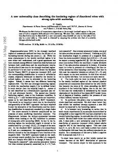
two critical exponents, γ and δ, which describe the response properties. The index γ describes the divergence of the susceptibility, which can be written as ∂Asat (θ) χ(θ) = , (33) ∂F1 F1 →0 for m = 1. The results are shown by triangles (θ < 0) and circles (θ > 0) in Figure 5. Computation of χ at some θ requires at least 5 values of Asat corresponding to the given F1 . At the same time, F1 must small enough to avoid the effects of Asat depending nonlinearly on F1 . Again it requires extensive calculation of all quantities to high accuracy. In both cases χ(θ) is approximated by χ± ∝ |θ|−γ± ,

which describes the amplitude of a weakly-unstable perturbation in a one-species Vlasov-Poisson system [10]. According to (37) the maximum amplitude ysat at y˙ = 0 scales with γL as ysat = γL2 . On the assumption that at γL . 0 the system responds linearly to an external pump ∂F , one can obtain the response ∂y to ∂F as γL ∂y −

χ− ≈ 2χ+ .

(35)

This difference, as well as the appearance of scaling (1) and (32) with β = 2 instead of β = 1/2 can be explained if one takes into account the difference between the Landau-Ginzburg Hamiltonian κ2 µ2 2 λ |∇φ|2 + |φ| + (|φ|2 )2 , 2 2 4! 2

2 3ysat ∂y + ∂F = 0. 4γL3

(38)

However, equation (37) is not valid at γL < 0 since it predicts unlimited growth instead of damping in this case. At small initial perturbation y0 the correct evolution is given by the linear equation y˙ = γL y, and the susceptibility χ = ∂y/∂F is

(34)

and γ− = 1.028 ± 0.025 for θ < 0, γ+ = 1.033 ± 0.016 for θ > 0 giving γ− ≈ γ+ = γ ≈ 1. These exponents are very close to the corresponding results for [19], because χ is the only linear coefficient, and this is common to both wave-particle and wave-wave interactions. The exponent γ is the same as for the mean-field thermodynamic models but, opposite to thermodynamics, the response is stronger at θ < 0 than at θ > 0, as Figure 5 shows. The susceptibilities are

HLG =

FIG. 5: Plot of χ vs. |θ|. Circles (θ > 0) and triangles (θ < 0) represent experimental data, the dashed lines are the power– law best fits.

χ+ = γL−1 ,

(39)

χ− = 2γL−1 .

(40)

and at γL > 0

At the critical point θ = 0 (or γL = 0) the response is described by another critical exponent δ 1/δ

Asat ∝ F1 .

(41)

The results of simulation are plotted in Figure 6, giving δ = 1.503 ± 0.005. This exponent cannot be obtained by the previous simple assumption from (37) because of its singularity at γL = 0. IV.

SCALING LAWS AND SYMMETRIES OF THE MODEL

(36)

[where φ is the order parameter and µ ∼ (T − Tcr )/Tcr ], which describes the Ising universality class, and the equation   1 (37) y˙ = y γL − 3 y 2 + O(y 4 ) , 4γL

The remarkable property of the critical exponents γ, β, and δ is that they satisfy the Widom equality (7) [14] with high accuracy. In thermodynamics the Widom equality is a consequence of the scaling of the Gibbs free energy under the transformation G(λaǫ ǫ, λaB B) = λG(ǫ, B) ,

(42)

6 This situation differs significantly from thermodynamics where 1 − aB β= . (47) aǫ This expression rescales the normalized distance from the critical point with external field B. Substituting Asat according to the power law (31) for 2 the order parameter to vsep = 4Asat ∝ (−θ)β one can obtain (assuming av = 1) FIG. 6: Asat as a function of F1 . Circles represent experimental data, the dashed lines are the power-law best fit.

from which it can be derived straightforwardly [1]. The functions which comply the condition (42) are called generalized homogeneous functions, and the condition itself is termed a homogeneity condition. The nature of this scaling for the marginally-stable Vlasov-Poisson system is clear from Figure 4, where the distribution function f (x, v, t) is plotted at the moment t = tsat . The remarkable property of the critical dynamics is the topological equivalence of the phase portraits for different θ: at the moments of saturation t1 and t2 corresponding to θ1 and θ2 we can write f (x, λav v, θ1 , t1 ) = λf (x, v, θ2 , t2 ) ,

(43)

fm (λav v, θ1 , t1 ) = λfm (v, θ2 , t2 ) ,

(44)

or

for the Fourier component. Transformation between t1 , θ1 and t2 , θ2 can be written as t′ → λat t, θ′ → λaθ θ, so fm (λat t, λav v, λaθ θ) = λfm (t, v, θ).

(46)

The critical exponents β, γ, and δ can be expressed via the scaling exponents av , aθ , and aF1 from which the Widom equality for the Vlasov-Poisson system can be proved directly (Appendix A). They also provide a deep insight into symmetry properties of the system. According to expression (A4) β=

1 + av , aθ

rescaling the parameter of θ (or growth rate) also rescales the distribution function f (t, v, x) in the v-direction.

(48)

from which the scaling exponent is aθ = 1 for β = 2 (aθ = 4 for β = 1/2). Remarkably, the two different processes – the linear growth of an unstable perturbation due to the resonant wave-particle interaction and the subsequent nonlinear saturation of this process due to particle trapping are interrelated. While there is no thermodynamic equilibrium in the collisionless system considered here, one can define the quantity which describes the response of the system to external thermal perturbation, just as the specific heat capacity describes the response of a thermodynamic system to heat transfer, C = δQ/dT . For the case, considered here δQ dV C= ≡ , (49) dθ dθ where V is the potential energy of the system. To calculate the specific heat capacity, Vsat corresponding to Asat is used. The critical exponent α can be calculated straightforwardly from (49) and (31). Because perturbations m > 1 are negligible for |θ| ≪ 1, Vsat ∝ Asat Φsat , where Φsat = −Asat ; i.e., Vsat ∝ − (− θ) 2β , θ < 0, and the heat capacity is given by

(45)

A weak external pump in the form F (x) = F1 cos(k1 x+ ϕ) creates a similar topology in the phase space because of the same mechanism of the saturation and adds an additional variable to the distribution function. The transformation can be written as F1′ → λaF1 F1 . Finally for fm = fm (t, v, θ, F1 ) we can write the homogeneity condition as fm (λat t, λav v, λaθ θ, λaF1 F1 ) = λfm (t, v, θ, F1 ).

vsep ∝ (−θ)1/aθ ,

C ∝ −(− θ) −α ,

(50)

α = −(2β − 1).

(51)

where

The scaling law (51) can be proven using the homogeneity condition (46) (Appendix A). Remarkably, the critical exponent α does not depend on the sign of Poisson’s equation, and result is the same for the plasma case. Unlike thermodynamics where the relation between exponents β, γ, and α is given by Rushbrooke’s equality, α + 2β + γ = 2, the scaling law (51) does not contain the critical exponent γ. Nevertheless, the set of critical exponents α = −2.990 ± 0.006, β = 1.995 ± 0.003, and γ = 1.031±0.021 satisfy Rushbrooke’s equality with high accuracy. V.

CORRELATION EXPONENTS

The correlation function of fluctuations for the field ∂Φ (52) E=− ∂x

7 can be found from the fluctuation-dissipation theorem [28] as hE 2 iωk =

T Im[ε(ω, k)] , 2πω ε2

(53)

[29], where the permittivity ε is given by (24). Relation (53) can be integrated using the Kramers-Kronig dispersion relations, and in the static limit ω → 0 (53) becomes   1 4πσ 2 2 , (54) 1− hE ikm = mp kB ε(0, km ) where kB is the Boltzmann constant and mp is the particle mass. This equation can be rewritten as hE 2 ikm = −

4π σ 2 , mp kB θm

(55)

where θm =

as

σ 2 − σJ2 (m) . σJ2 (m)

(56)

The susceptibility χ can be written in terms of hE 2 ik1 χ = hE 2 ik1 ∝ θ−γ ,

(57)

γ = 1. The combination of σ and ω1 gives the characteristic length for the system from the dispersion relation (25) σ , ω1

(58)

ξ ∝ θ−ν ,

(59)

ξ = 2π or, in terms of θ,

as θ → 0. Therefore the critical exponent that characterizes the correlation length is ν = 1. The correlation function hE 2 ik1 can be rewritten in terms of kξ = ξ −1 as hE 2 ik1 ∝ kξ2−η ,

(60)

where η is another critical exponent which characterizes the correlation function. On the other hand, using (59) one can rewrite this expression as hE 2 ik1 ∝ θ−ν(2−η) ,

(61)

and, taking into account (57), θ−γ ∼ θ−ν(2−η) ,

(62)

from which finally we obtain the equality γ = ν(2 − η).

(63)

The last equality is known as Fisher’s equality and gives the last critical exponent, η = 1.

VI.

RELATION WITH OTHER UNIVERSALITY CLASSES

The correlation function (55) looks rather counterintuitive, since at θm > 0 (damping waves), one has hE 2 ikm < 0, and the noise is imaginary. Nevertheless, this unusual situation has an analog – for particle-particle annihilation reactions of the type Y + Y → 0 (corresponds to equation dn/dt = −an2 , a > 0), Y → 0 (dn/dt = −an) the correlation function is also negative because of anticorrelation of particles [30]. In the case θm > 0 the amplitude Am → 0 as t → 0. It is also shown that the criticality due to these annihilation processes belongs to a certain universality class which is different from the Ising universality class [30, 31] and therefore is not described by the Landau-Ginzburg Hamiltonian (36). Another unusual quantity is the correlation length ξ and the wavevector kξ = ξ −1 , whose use allows us to establish the validity of Fisher’s equality for the collisionless system, studied here. It is not related to the size of the system L but to the fluctuations in the system which determine an average path of correlated motion of particle in presence of these fluctuations. As the system approaches the threshold, fluctuations become correlated since the characteristic time of correlations ω −1 ∼ θ−1 diverges as θ → 0. This behavior is analogous to thermodynamic systems where the correlation length is the only relevant scale near the critical point as ǫ → 0. To demonstrate that the criticality in the VlasovPoisson system belongs to a different class, let us compare the critical exponents corresponding to the Jeans instability in a self–gravitating hydrodynamical system [27], using the same approach. The dispersion relation for this system is 2 2 ωm = c2s km − 4πGρ0 ,

(64)

2 2 ωm = (c2s − c2m )km ,

(65)

or

2 where c2m = 4πGρ/km is the critical velocity of sound, 2 corresponding to ωm = 0. As for kinetic case if c2 > c21 = c2cr , there are no unstable modes, and the correlation length is

ξh =

2πcs 1 −1/2 ∼ θf , ω1 k1

(66)

where θf = (c2s − c2cr )/c2cr is the reduced sound velocity in a fluid. Here we have the mean-field exponent νf = 1/2. Assuming m = 1 and dividing the both sides of dispersion relation (65) on c2s one can obtain the correlation function as !−1 kξ2h (2) Gh (kξh , θf ) = . (67) − θf k12 This is the propagator of Euclidean theory or of the scalar boson field [13] from which the Landau mean-field theory follows automatically.

8 On the other hand dispersion relation (25) for the collisionless case gives !−1 r 2 k ξ G(2) (kξ , θ) = i −θ . (68) π k1 For collisionless systems the propagator thus corresponds to the vector fermionic field and describes a different class of critical phenomena. In the language of quantum field theory the parameters θf and θ are bare masses. Since G(2) (k, 0) ∝

1 k 2−η

,

(69)

from (67) and (68) one can obtain η = 0 for the case of hydrodynamics and η = 1 for collisionless system. VII.

HYPERSCALING LAWS

The approach assumed in the previous section allows us to establish the hyperscaling law for the VlasovPoisson system which involves the dimensionality d along with critical exponents like Josephson’s law (8). Using propagator (68) which is the potential energy, the specific heat capacity C in d-dimensional space at θ → 0 can be obtained as Z ∂ dd kξ G(2) (kξ , θ) . (70) C∼ ∂θ which gives C ∝ ξ 2−d .

(71)

With relation (59), (71) becomes C ∝ θ−ν(2−d) .

(72)

Taking into account the scaling law (50) for the specific heat capacity C one can obtain the hyperscaling relation which interrelates the exponents α, ν, and the dimensionality d α = ν(2 − d) .

(73)

The last equality reveals d = 2 as the upper critical dimensionality for the Vlasov-Poisson system since the heat capacity becomes divergent if d < 2, thus indicating the importance of fluctuations in the critical area. It also shows that the dimensionality corresponding to the critical exponents α = −3 and ν = 1 is d = 5, fluctuations at θ ≈ 0 are insignificant, and therefore α = −3, β = 2, γ = 1, ν = 1, and η = 1 are the mean-field exponents. The use of the scalar field propagator (67) instead of (68) gives α = ν(4 − d) ,

(74)

and at α = 0 the upper critical dimensionality is dc = 4 which is the Landau mean-field theory case for the Ising

universality class. However, relation (74) is not valid for the Vlasov-Poisson system because of its different propagator. On the contrary to relations (73) and (74) which are valid for specific propagators (67) and (68), Josephson’s law (8) is universal for all cases considered. With exponents ν = 1 and νf = 1/2 it gives dc = 2 and dc = 4 as the upper critical dimensionalities for the collisionless and hydrodynamic cases, respectively, and d = 5 for the exponents of the Vlasov-Poisson system calculated here. Without going into details here, we note that this universality appears because the fundamental description is given by the same functional integrals in both cases. In particular for the free scalar bosonic field (no interactions) the partition function is  Z  Z d ZG = Dφ exp − d xH0 , where H0 is the Landau-Ginzburg Hamiltonian HLG (36) without quadratic term. In the fermionic case the Lagrangian for a Dirac spinor field is used instead of H0 . VIII.

CONCLUSIONS

We have studied numerically and analytically a model Vlasov–Poisson system near the point of a marginal stability. The most important finding is that the criticality of the Vlasov–Poisson model studied here belongs to a universality class described by the propagator corresponding to a fermionic vector field. This finding is in striking contrast with the previous critical phenomena studies concerning systems whose criticality belongs to universality classes corresponding to the scalar bosonic fields, like the Ising universality class. This fundamental discrepancy emerges from the qualitative difference between objects considered: the Landau–Ginzburg Hamiltonian (36) takes into account spatial variations of the order parameter via the local differential operator ∇, whereas the integro–differential operator for the Vlasov–Poisson model acts on the distribution function containing the additional dimension of velocity. We have calculated numerically the critical exponents which describe the critical state of the model and established analytically that these exponents and the dimensionality are interrelated by the scaling and hyperscaling laws like the Widom, Rushbrooke, and Josephson laws at the formal dimensionality d = 5. The upper critical dimensionality is dc = 2 and since d > dc the calculated exponents are the mean-field exponents, different from those which one might expect the Landau–Weiss set of critical exponents corresponding to the Ising mean–field model where dc = 4. This is related to the higher dimensionality of the Vlasov–Poisson kinetic problem associated with the velocity space and to the type of the criticality of the Vlasov-Poisson systems, which belongs to a universality class different from the Ising universality class.

9 The critical exponents we have found here are α = −3, β = 2, γ = 1, δ = 1.5, ν = 1 and η = 1. The difference between this set and the set α ≈ −2.814, β ≈ 1.907, γ ≈ 1, δ ≈ 1.544, ν = 1 and η = 1 [19] is because Asat is about 50 times larger for the latter case, thus causing wave-wave interactions to dominate, thereby yielding a different universality class. More important, the later exponents satisfy scaling laws at fractal dimension d ≈ 4.68 indicating reduced dimensionality because wavewave interactions have fewer degrees of freedom than wave-particle ones [21].

Equations (A4)-(A6) can be rewritten in matrix form as WA = X ,

(A8)

where A = [aθ , av , aF1 ]T , X = [1, −1, −δ]T , and the matrix W is   β −1 0 W =  γ 1 −1  . (A9) 0 δ −1 The determinant of W is

Acknowledgments

det W = −β + δβ − γ ≡ 0 .

This work was supported by the Australian Research Council and a University of Sydney SESQUI grant.

Using (A6) to eliminate av , the system (A8) can be reduced to

APPENDIX A: RELATION BETWEEN THE SCALING AND CRITICAL EXPONENTS

From the homogeneity condition (46) fm (λat t, λav v, λaθ θ, λaF1 F1 ) = λfm (t, v, θ, F1 ) ,

(A1)

1 aF = 0 , δ 1   1 − 1 aF1 = 0 , + δ

βaθ −

(A11)

γaθ

(A12)

for which solution exists only if the Widom equality γ = β(δ − 1) holds. Therefore aθ and aF1 can be formally considered as the eigenvectors of W whose eigenvalue is λ = 0. In particular

for ρm components by integration over v, one has −av

λ

aθ

at

aF1

ρm (λ t, λ θ, λ F1 ) = λρm (t, θ, F1 ).

For any two Asat = ρ1 (tsat ) and write

A′sat

=

ρ1 (t′sat )

λ−av Asat (λaθ θ, λaF1 F1 ) = λAsat (θ, F1 ).

(A2)

one can (A3)

1/aθ

Assuming λ = (−1/θ) , the critical exponent β can be rewritten in terms of the scaling exponents av and aθ as β=

1 + av . aθ

(A4)

1 aF1 β+γ

(A13)

which indicates that rescaling of the distribution function under an external pump is equivalent to rescaling due to the field which appears for nonzero order parameter. APPENDIX B: RUSHBROOKE’S LAW FOR VLASOV–POISSON SYSTEM

The heat capacity can be formally defined as C=

dV δQ ≡ , dθ dθ

(B1)

−av − 1 + aF1 , aθ

(A5)

aF1 , 1 + av

(A6)

Vsat ∝ A2sat .

δ=

and the Widom relation follows from (A5) straightforwardly: γ=

aθ =

where V is the potential energy of the system. To calculate the specific heat capacity, Vsat corresponding to Asat is used. Because perturbations m > 1 are negligible for |θ| ≪ 1, Vsat ∝ Asat Φsat , where Φsat = −Asat , and

In the similar way for γ and δ one can write γ=

(A10)

−av − 1 + aF1 1 + av aF = − + 1 aθ aθ aθ = −β + βδ = β(δ − 1) .

(A7)

(B2)

From (A3) one can obtain ∂ −2av 2 ∂ 2 2 Asat (λaθ θ, λaF1 F1 ) = λ λ Asat (θ, F1 ), (B3) ∂θ ∂θ or ∂ 2 ∂ −2av −2 2 λ Asat (λaθ θ, λaF1 F1 ) = A (θ, F1 ) . (B4) ∂θ ∂θ sat

10 Assuming λ = θ−1/aθ and F1 = 0, Equation (B4) can be rewritten as ∂ 2 ∂ (2av +2)/aθ 2 [θ Asat (−1, 0)] = A (θ, 0), ∂θ ∂θ sat

Equation (B5) has the form of the power law, C(θ, 0) ∝ θ−α , with

(B5)

or ∂ 2 2av + 2 2 Asat (−1, 0) θ(2av +2)/aθ −1 = A (θ, 0), aθ ∂θ sat (B6)

α = −2

av + 1 + 1 = −2β + 1. aθ

(B8)

or (2av +2) 2av + 2 2 −1 = C(θ, 0). Asat (−1, 0) θ aθ aθ

(B7)

[1] H. E. Stanley, Introduction to Phase Transitions and Critical Phenomena (Clarendon, Oxford, 1971). [2] L. D. Landau and E. M. Lifshitz, Statistical Physics (Pergamon, Oxford, 1980) [3] E. Frieman, S. Bodner, and P. Rutherford, Phys. Fluids 6, 1298 (1963). [4] B. C. Fried, C. S. Liu, R. W. Means, and R.Z. Sagdeev, Plasma Physics Group Report PPG-93, University of California, Los Angeles, 1971 (unpublished). [5] M. B. Levin, M. G. Lyubarsky, I. N. Onishchenko, V. D. Shapiro, and V. I. Shevchenko, Sov. Phys. JETP 35, 898 (1972). [6] L. D. Landau, J. Phys. 10, 25 (1946). [7] J. E. Marsden and M. McCracken, The Hopf Bifurcation and Its Applications (Springer-Verlag, New York, 1976). [8] V. Latora, A. Rapisarda, and S. Ruffo, Phys. Rev. Lett. 80, 692 (1998). [9] A. Simon and M. Rosenbluth, Phys. Fluids 19, 1567 (1976). [10] J. D. Crawford, Phys. Plasmas 2, 97 (1995). [11] J. Denavit, Phys. of Fluids 28, 2773 (1986). [12] J. Candy, J. Comp. Phys. 129, 160 (1996). [13] D. J. Amit, Field theory, the renormalization group and critical phenomena (World Scientific, Singapore, 1984). [14] B. Widom, J. Chem. Phys. 41, 1633 (1964). [15] B. D. Josephson, Proc. Phys. Soc. 92, 269, 276 (1967). [16] D. Stauffer and A. Aharony, Introduction to percolation theory (Taylor & Francis, London, 1994).

The last relation corresponds to Rushbrooke’s equality α + 2β + γ = 2 at γ = 1.

[17] C. Domb, Adv. Phys. 9, 45 (1960). [18] N. Goldenfeld, Lectures on phase transitions and the renormalization group (Addison-Wesley, Reading, Massachusetts, 1992). [19] A. V. Ivanov, Astrophys. J. 550, 622 (2001). [20] P. A. Robinson, Rev. Mod. Phys. 69, 507, (1997). [21] S. V. Vladimirov, V. N. Tsytovich, S. I. Popel, and F. Kh. Khakimov, Modulational Interactions in Plasmas (Kluwer, Dordrecht, 1995). [22] S. Ichimaru, D. Pines, and N. Rostoker, Phys. Rev. Lett. 8 231 (1962). [23] B. D. Fried and S. D. Conte, Plasma Dispersion Function: The Hilbert Transform of the Gaussian (Academic Press, New York, 1961). [24] C. Z. Cheng and G. Knorr, J. Comput. Phys. 22, 330 (1976). [25] R. K. Mazitov, Zh. Prikl. Mekh. Fiz. 1, 27 (1965). [26] T. M. O’Neil, J. H. Winfrey, and J. H. Malmberg, Phys. Fluids 14, 1204 (1971). [27] J. Jeans, Astronomy and Cosmogony (University Press, Cambridge, 1928). [28] H. B. Callen and T.A. Welton, Phys. Rev. 83, 34 (1951). [29] R.J. Kubo, J. Phys. Soc. Japan 12, 570 (1957). [30] M. J. Howard and U. C. T¨ auber, J. Phys. A: Math. Gen. 30, 7721 (1997). [31] B.P. Lee, J. Phys. A: Math. Gen. 27, 2633 (1994).