many application domains (e.g. e-business, switching systems) software sys- ... The visualizations should be well suited to represent large software struc- tures ...
CrocoCosmos – 3D Visualization of Large Object-Oriented Programs Claus Lewerentz and Andreas Noack Brandenburg Technical University at Cottbus, Computer Science Department, Software Systems Engineering Research Group, Postbox 10 13 44, D-03013 Cottbus, Germany
1
Introduction
Software belongs to the most complex human-made artefacts. The size and complexity of programs has constantly grown over the last years. Today in many application domains (e.g. e-business, switching systems) software systems with millions of lines of code are constructed. They consist of many thousands of components and subsystems. Prefabricated frameworks and component technology make it possible to quickly build very large programs which typically go through a long lasting evolution process with adaptations and extensions of the existing code. Such reengineering and maintenance activities require good support for program analysis and understanding. In the context of program comprehension typical questions are “How good is the quality of the program with respect to maintainability?”, “Where are the most critical parts?”, “What is the overall structure of the system?”, “How are particular parts interdependent?” (cf. [19], [21]). One way to support program comprehension is software visualization based on automatically extracted information about the internal program structure and on derived software metrics data [14]. Typical examples are inheritance or call graphs depicting program entities like subsystems, classes, or functions, and inheritance or call relations between them. There are many other approaches visualizing different aspects of software systems (cf. [12]). For an effective use of software visualizations in the context of program comprehension and reengineering of real-world systems they have to fulfil some important requirements: 1. Geometric properties of a system’s visualization have to allow for a valid interpretation with respect to the system properties. The size and geometric distance of graphical entities representing particular program elements, for instance, has to have sound correlation with the underlying program structure and thus an interpretation in the problem domain. This provides a basis for producing visual patterns that are clearly related to structural patterns of intended or undesired constructions. 2. The visualizations should be well suited to represent large software structures, i.e. high resulting data volumes. Typical software in industrial development projects nowadays consists of 105 -107 lines of source code orga-
2
Claus Lewerentz and Andreas Noack
nized in 104 -105 functions in 103 -104 classes or files, contained in 102 -103 packages or subsystems. Thus, the visualization approach has to scale well and to support hierarchical visual structures with robust transitions between different hierarchy levels. 3. The visualization technique has to be flexible and adaptable in order to provide means for the creation and exploration of different views which appropriately support specific analysis and comprehension tasks.
Fig. 1. Schema for the representation of object-oriented programs
In our metrics-based software analysis approach [21,13] we use a product abstraction of object-oriented programs that results in large attributed graph structures with several thousand vertices and tens of thousands of edges representing different logical views on a software system. Figure 1 shows a simplified schema for the internal representation of object-oriented programs on the level of subsystems and classes with the relations for class nesting, method call, attribute access, and inheritance. On this level we abstract from the code structure within methods and represent particular instruction level information (e.g. the number of lines of code for a method or a class) by metrics values which are part of the schema as attributes. Views on this schema correspond to hierarchical call, use, or inheritance graphs. The CrocoCosmos tool creates three-dimensional visual representations of the graph structures resulting from the instantiation of this schema for large
CrocoCosmos – 3D Visualization of Large Object-Oriented Programs
3
Fig. 2. Example visualization
programs. As illustrated in Fig. 2, vertices represent program entities and colored edges represent relations of different types. Particular properties of the individual entities are encoded by geometrical vertex properties and edge directions are encoded by color transitions. The positions of the vertices in 3D space reflect the relational structure of the visualized program. The use of 3D space instead of 2D space is motivated by the experience that the additional degree of freedom in many cases drastically enhances the spatial unfolding of large graph structures. Section 3 explains and discusses our layout approach in detail.
2
Applications
CrocoCosmos is part of a comprehensive experimental software analysis tool set to support analysis, comprehension, and quality assessment of large objectoriented programs. Based on parsing, structure extraction and transformation, and metrics calculation, different analysis views of programs are created and used for interactive exploration (cf. Fig. 3). The 3D-graph view is one particular view which mainly supports overall structure recognition and the visual detection of potentially anomalous program constructions like overly complex inheritance structures or repetitive structures caused by code clones. The visualizations were used in several industrial case studies for software quality assessment, review preparation and reengineering support (cf. [21,15]). The experiences show that the visualizations complement other analysis data, tabular views and browsing structures in a very useful way. Their particular strength is that the 3D-graphs provide overall pictures as well as detailed structural insights, that are difficult to derive from the other views. In several cases the 3D-visualizations showed very directly unexpected structures which were clearly related to complex and cumbersome internal structures of the analyzed software (cf. Sect. 5.2 for examples). It is, however, necessary to learn to interpret the visual structures and to relate visual patterns to desired or problematic program structures. There is still substantial empirical work to be done.
4
Claus Lewerentz and Andreas Noack
Fig. 3. Analysis and visualization of software systems
3
Algorithms
CrocoCosmos uses force-directed methods to draw graph models of programs. This choice is motivated by the requirements for effective software visualizations listed in Sect. 1. Consider the third requirement, adaptability to different views on software systems. This means drawing graphs with different graph-theoretic properties. Inheritance graphs, for instance, are acyclic and very sparse, while call graphs often have large strongly connected components and many times more edges. Force-directed methods are easily adaptable to different kinds of graphs. In general, they have two parts: an energy model, and an algorithm for finding a state of minimum total energy. (Alternatively, the model may be defined as force system and the algorithm searches for an equilibrium configuration where the total force on each vertex is zero.) The drawing criteria are explicitly specified in the energy model and can be changed without modification of the algorithm. Section 4.5 of the Technical Foundations Chapter gives an introduction to force-directed methods and lists some popular force and energy models. However, these models are not well suited for some important graphs of software systems. In this section we develop an energy model for the drawing of reference graphs, which include call, attribute access, and inheritance relations. Therefore we state some graph-theoretic properties of reference graphs, derive criteria for their drawings, discuss existing energy models with respect to these criteria, and formalize the criteria to obtain a new energy model. Finally we address the first requirement of Sect. 1 by proving the interpretability of distances in the drawings of this energy model.
CrocoCosmos – 3D Visualization of Large Object-Oriented Programs
3.1
5
Properties of Reference Graphs
In general, the vertices of a reference graph are structural entities of a software system like methods, classes or subsystems. There is a directed edge from a vertex u to another vertex v if and only if a method of entity u calls a method of entity v, or a method of u uses an attribute of v, or a class of u directly inherits from a class of v. Including inheritance and attribute usage adds relatively few edges, so most of the following also applies to call graphs. For clarity of presentation, we simplify the notion of a reference graph in two respects: Firstly, we consider the edges as undirected. In our visualizations, the direction and the type of the edges is only indicated by their coloring (cf. Sect. 4), and does not affect the positions of the vertices. Secondly, we treat the components of the reference graph separately. So in the following, reference graphs are undirected, connected, simple graphs. Table 1 shows some properties of reference graphs of four software systems. For a graph G = (V, E) and using the notations of the Technical Foundations Chapter, these properties are defined as follows: • Average degree: • Density:
1 |V |
2|E| |V |(|V |−1) ,
� v∈V
deg(v) =
2|E| |V | .
the fraction of the possible edges that actually exist.
– Graph-theoretic distance: The length of the shortest path connecting two vertices u and v is their graph-theoretic distance δ(u, v). We stress graphtheoretic to preclude confusion with the Euclidean distance in the drawing. � • Average graph-theoretic distance: |V |(|V1 |−1) u,v∈V,u�=v δ(u, v). • Diameter: max{δ(u, v) | u, v ∈ V }, the maximum graph-theoretic distance. – Clustering coefficient γ(u) of a vertex u with deg(u) ≥ 2 [22]: �� �� 2 � {v, w} ∈ E | v, w ∈ adj(u) �, deg(u)(deg(u)−1)
the fraction of those possible edges between neighbors of u which actually exist in the graph. � 1 • Clustering coefficient of a graph: |{v∈V | deg(v)≥2}| v∈V,deg(v)≥2 γ(v), the average clustering coefficient of all vertices with at least two neighbors. In all four reference graphs of Table 1 more than 90 percent of the vertices have at least two neighbors. Three observations are of particular importance for the drawing of reference graphs: 1. The average distance of vertices and the diameter are very small compared to the number of vertices. This raises the problem how of to avoid drawing many vertices and edges in very small areas or volumes.
6
Claus Lewerentz and Andreas Noack
Number of Vertices 170 539 662 1508
Number of Edges 691 2239 3690 9759
Average Degree 8.13 8.31 11.15 12.94
Density 0.0481 0.0154 0.0169 0.0086
Average Diameter Clustering Distance Coefficient 2.71 5 0.247 3.39 8 0.382 2.88 11 0.334 2.74 10 0.275
Table 1. Properties of the reference graphs of four software systems
2. The clustering coefficients are high. While in random graphs (i.e. graphs where every pair of different vertices is connected with equal probability) the clustering coefficient is approximately equal to the density, it is much higher in the four reference graphs. So reference graphs probably have natural clusters, i.e. subsets of vertices with many internal edges (high cohesion) and few edges to outside vertices (low coupling). These natural clusters should be apparent in the visualization. 3. The average degree is high. Drawings of graphs with that many edges often appear cluttered. So ideally the viewer would know where edges are without actually seeing them. This can be partially achieved by indicating the number of edges connecting two subgraphs by the closeness of the subgraphs. 3.2
Discussion of Existing Energy Models
This section explains why most popular force and energy models, in particular those mentioned in Sect. 4.5 of the Technical Foundations Chapter, are not well suited to drawing reference graphs. For a more detailed discussion see [17]. An energy model specifies what is considered a good drawing. More precisely, for a given graph, a drawing with high total energy is considered worse than a drawing with lower total energy. Force and energy are just two different perspectives on the same problem: Force is the negative gradient of energy, thus an equilibrium state of a force model is a local minimum of energy. We prefer the perspective of energy minimization because local minima can have high energies and therefore give bad drawings compared to the global minimum. Section 4.5 of the Technical Foundations Chapter introduces the models of Eades [6], Fruchterman and Reingold [9], Frick et al. [8], and Davidson and Harel [5], which are sums of a term for the spring energy and a term for the repulsion energy. (The model of Davidson and Harel has two additional terms.) These terms formalize a popular criterion for good drawings: Adjacent vertices should generally be closer than non-adjacent vertices. This conforms to our goal to make dense subgraphs visually apparent, and thus our energy model (introduced in Sect. 3.4) has the same form.
CrocoCosmos – 3D Visualization of Large Object-Oriented Programs
7
But the particular terms differ, because the energy models from the Technical Foundations enforce an additional property of the drawing: uniform edge lengths. Strong forces act between adjacent vertices towards some fixed desired edge length (which is a parameter of the models), while the repulsive forces between vertices decay rapidly with growing distance. This results in distances between adjacent vertices which are almost independent of global properties of the graph. Uniform edge lengths are not desirable in drawings of reference graphs. Table 1 shows that the average graph-theoretic distance of two vertices is only about 3. The result of drawing such graphs with uniform edge lengths are hundreds of edges of length 1 in a circle or sphere of diameter 3 – a clutter that does not reveal much about the structure of the software system (except its small diameter). Section 5.1 illustrates this with a comparison of drawings of the Fruchterman-Reingold model and our energy model. The same argument rules out the energy model of Kamada and Kawai [11] (also introduced in Sect. 4.5 of the Technical Foundations Chapter) which aims at Euclidean distances of the vertices being proportional to their graph-theoretic distances. All mentioned force and energy models easily generalize to different desired edge lengths for each edge, i.e. to the drawing of graphs with weighted edges so that the desired length of every edge depends on its weight. Further energy models serving this purpose were proposed in the literature on information visualization [4,7] and multidimensional scaling (e.g. [2]). So our first approach was to apply a similarity measure to determine the desired distance of every pair of vertices, and to compute drawings that preserve these distances at least on an ordinal scale [14,20]. One requirement for the desired distances is that vertices of the same cluster of the graph should be closer to each other than vertices of different clusters. So specifying desired distances requires knowledge of the clusters of the graph, but most variants of the graph clustering problem are N P-hard. (See [1,18] for surveys on graph clustering.) In the following, we introduce an energy model that does not take desired edge lengths as input parameter. Instead, it is only the interplay of attractive and repulsive forces which reveals the global structure of the graph. In this respect our approach is similar to that of Hendley et al. [10] who, however, did not publish their force model and an analysis of its properties. The main advantages over energy models which aim at preserving given desired distances are: 1. Knowledge about the clusters of the graph is not required as input, but provided as output. 2. Instead of hoping that the given desired distances are preserved in the drawing, it can be proved that the distances in the minimum energy drawing are interpretable.
8
Claus Lewerentz and Andreas Noack
3.3
The Cut Ratio as a Measure of Coupling
In this subsection we define the cut ratio of two clusters and explain why its inverse is an appropriate distance of these clusters in the drawing. In the next subsection an energy function is introduced whose minimization produces a drawing in which clusters have this distance – without taking any explicit information about clusters as input. Let V1 and V2 be two nonempty, disjoint subsets of the set of vertices V . Then the cut that separates V1 and V2 is the set of edges connecting both subsets: cut(V1 , V2 ) = E[V1 ∪ V2 ] \ (E[V1 ] ∪ E[V2 ]) The ratio of this cut is the fraction of the possible edges between V1 and V2 which actually occur: ratio(V1 , V2 ) =
| cut(V1 , V2 )| |V1 | · |V2 |
The ratio of a cut was introduced as quality metric for partitions of circuits by Wei and Cheng [23], and was more recently applied as a metric for coupling in the clustering of call graphs [16]. Because it is normalized with respect to the number of possible edges, its interpretation is independent of the size of V1 and V2 . If, for example, |V1 | = |V2 | = 2, then a cut size of 4 means maximum coupling. If |V1 | = |V2 | = 10, the same cut size means loose coupling. This is reflected by the ratio of the cuts which takes the maximum possible value 1 in the first case and the near-minimum value 0.04 in the second case. Wei and Cheng [23] present the same idea from the opposite perspective: For all cuts of a random graph the expected value of the ratio is equal, while the expected size of the cuts strongly depends on the sizes of the separated sets of vertices. Suppose ratio(V11 , V12 ) � ratio(V1 , V2 ) and ratio(V21 , V22 ) � ratio(V1 , V2 ) for all partitions of V1 into non-empty sets V11 and V12 and all partitions of V2 into non-empty sets V21 and V22 , i.e. V1 and V2 are clusters with high cohesion and low coupling. Then the intra-cluster distances in the drawing should be small, and the distance between V1 and V2 should be much greater and depend on the coupling of V1 and V2 . Since ratio(V1 , V2 ) measures the 1 is an appropriate distance of V1 and V2 : coupling, ratio(V 1 ,V2 ) • Higher couplings imply lower distances. More precisely, doubling the number of edges between V1 and V2 halves their distance. • If no edge connects V1 and V2 , their distance is infinite. This causes no problems when different components of a graph are treated separately. • The minimum distance is 1, so even strongly coupled subgraphs are not drawn at the same position. At the same time, using the inverse ratio of the cut as distance also ensures small intra-cluster distances, because the ratios of the cuts that separate a cluster are high.
CrocoCosmos – 3D Visualization of Large Object-Oriented Programs
3.4
9
The LinLog Energy Model
In the LinLog energy model , the total energy of a drawing is � � ||pu − pv || − ln ||pu − pv || U= {u,v}∈E
{u,v}∈V (2)
where V (2) denotes the set {{u, v} | u, v ∈ V, u �= v} of all subsets of V with exactly two elements, and pv denotes the position of vertex v. To avoid infinite energies we always assume that different vertices have different positions. We now analyze the distances in a one-dimensional minimum LinLog energy drawing of a graph G = (V, E) where each vertex v has the position xv . The set of vertices V is partitioned into two sets V1 and V2 such that: 1. V = V1 ∪ V2 , V1 ∩ V2 = ∅, V1 �= ∅, V2 �= ∅, and 2. the vertices in V1 have smaller coordinates than the vertices in V2 : ∀v1 ∈ V1 ∀v2 ∈ V2 : xv1 < xv2 . Let us examine drawings where some d ∈ IR is added to the coordinates of all vertices in V1 , and which do not violate the second condition, i.e. d < min{xv | v ∈ V2 } − max{xv | v ∈ V1 }. The total energy of these drawings is the sum of the energy within each of the two subgraphs G[V1 ] and G[V2 ], and the energy between these two subgraphs: � � U (d) = |xu − xv | − ln |xu − xv | {u,v}∈E[V1 ]∪E[V2 ]
+
�
(2)
{u,v}∈V1
(|xu − xv | + d) −
{u,v}∈E\(E[V1 ]∪E[V2 ])
{u,v}∈V
(2)
∪V2
�
ln(|xu − xv | + d)
(2) \(V (2) ∪V (2) ) 1 2
By definition of the xv , this function has a global minimum at d = 0, so U � (0) = 0. � � � 1 U � (d) = �E \ (E[V1 ] ∪ E[V2 ])� − |xu − xv | + d (2) (2) {u,v}∈V (2) \(V1
�
0 = | cut(V1 , V2 )| −
(2)
{u,v}∈V (2) \(V1
(2)
∪V2
)
∪V2
)
1 |xu − xv |
Inserting the harmonic mean of the distances between V1 and V2 harm(V1 , V2 ) = �
|V1 | · |V2 | (2)
{u,v}∈V (2) \(V1
(2)
∪V2
1 ) |xu −xv |
we get |V1 | · |V2 | harm(V1 , V2 ) 1 |V1 | · |V2 | = harm(V1 , V2 ) = | cut(V1 , V2 )| ratio(V1 , V2 ) 0 = | cut(V1 , V2 )| −
10
Claus Lewerentz and Andreas Noack
So we have shown that wherever one cuts a one-dimensional minimum LinLog energy drawing of a connected graph into two non-empty subgraphs, the harmonic mean of the inter-subgraph distances equals the inverse ratio of the cut. Thus valid (and useful, see Sect. 3.1) inferences about the structure of the graph can be made from the positions of the vertices. The harmonic mean of the inter-subgraph distances is more appropriate than the arithmetic or geometric mean here because it weights small distances higher than large distances. This corresponds well to our intuitive notion of the distance of two subgraphs. If the intra-subgraph distances are much smaller than the inter-subgraph distances, the three means are roughly equal. Unfortunately, the result does not generalize to two- or higher-dimensional minimum energy drawings. However, we have neither theoretical nor empirical reasons to believe that it is seriously violated in practice. In particular, the one-dimensional case is a good approximation when the intra-subgraph distances are much smaller than the inter-subgraph distances. A more detailed analysis of the LinLog energy model and additional energy models for reference graphs can be found in [17].
4
Implementation
In the reference model of information visualization developed by Card et al. [3, Chap. 1], visualizations are considered as series of adjustable mappings from raw data to views of visual structures. This section describes the mappings of CrocoCosmos. 4.1
Data Extraction
The raw data of CrocoCosmos is the source code of an object-oriented program. The source code is mapped to an attributed nested graph (see Sect. 2.6 of the Technical Foundations Chapter for the definition of nested graphs) which is an instance of the schema depicted in Fig. 1: • Program entities, like methods, attributes, classes, files, and subsystems, are mapped to vertices of the graph. • The containment hierarchy of the program is mapped to the inclusion tree of the nested graph. The containment hierarchy includes the relations of methods and attributes to their containing class, of classes to their containing file, and of files und subsystems to their containing subsystem. • Other relations of program entities, mainly the “uses” relation between methods and attributes, the “calls” relation between methods, and the “inherits from” relation between classes, are mapped to directed edges. • The vertices of the graph are attributed with the values of metrics. Metrics map properties of program entities, like the size or the number of incoming and outgoing relations, to numbers. A particular set of metrics can be defined for the entities of each level of the hierarchy, i.e. methods, classes, files, subsystems and the whole system.
CrocoCosmos – 3D Visualization of Large Object-Oriented Programs
4.2
11
Level of Detail and Filtering
By choosing the level of detail and applying filtering mechanisms, the user defines a mapping from the nested graph to a graph without hierarchy. The level of detail can be set globally, and modified for each vertex individually by replacing it by its children and vice versa. For example, first showing the whole system at class level and then replacing a class by its methods and attributes results in a detailed view of this class in global context. Because the inclusion tree of the nested graph is not represented in the main visualization, CrocoCosmos provides an additional window that shows the containment hierarchy of the software system. This hierarchy window is closely linked to the main view. For example, clicking on a vertex in the hierarchy window focusses this vertex in the main view. The user also controls which vertices and edges of the chosen level of detail are included in the hierarchy-free graph and which are elided. This makes it possible to examine parts of a program in isolation, or to start with a few methods and explore how they are used by the remaining system. 4.3
Graph Layout
Force-directed layout algorithms attribute each vertex of the graph with a position in three-dimensional space. To adapt the drawing criteria to the properties of the graph and the purpose of the visualization, the user can choose between different energy models. For example, the Fruchterman-Reingold model produces readable layouts of inheritance graphs, while the LinLog model can reveal the structure of denser graphs like reference graphs. Section 3 discusses energy models in more detail. 4.4
Visual Mapping
The attributed graph is mapped to a visual structure as follows: • Vertices are mapped to volumes. • The shape, size and color of a volume represent the type and metric values of the corresponding vertex. For example, all methods can be displayed as stars, classes as spheres, files as cubes, and subsystems as pyramides. The diameter of the sphere representing a class can be defined by its number of methods, and all classes of the same subsystem might have the same color. All these mappings are controlled by the user. • Edges are mapped to straight lines. • The type and direction of an edge is shown by the color transition of the corresponding line. For example, a blue-yellow line indicates an inheritance relation from the entity at the blue end to the entity at the yellow end.
12
4.5
Claus Lewerentz and Andreas Noack
View Transformation
The user controls the point and direction of view by moving freely through the three-dimensional space. Viewpoints can be saved to return to them later. An additional way to change the view is focussing on a particular vertex by clicking on it in the hierarchy window, as mentioned in Sect. 4.2. When the mouse cursor is moved on a volume the name of the corresponding program entity is shown. Clicking on a volume opens a details-on-demand window with metric values or the source code of the corresponding entity.
5
Examples
The first subsection shows the ability of the LinLog energy model to reveal the structure of graphs for some pseudo-random graph with expected clusters. The second subsection sketches an analysis of a real-world software system with CrocoCosmos. 5.1
Random Graphs
The Figs. 4, 5 and 6 show drawings of pseudo-random graphs with clusters for our LinLog energy model (introduced in Sect. 3) and the wellknown Fruchterman-Reingold model (discussed in Sect. 3.2).1 In all figures, the LinLog model (left drawings) reveals the clusters more clearly than the Fruchterman-Reingold model (right drawings). The graph of Fig. 4 is a pseudo-random graph with eight clusters of 50 vertices each. The probability of an edge {u, v} is 0.2 if u and v belong to the same cluster and 0.01 otherwise. The eight clusters are clearly separated in the drawing for the LinLog model, but the borders of the clusters look fuzzy and some vertices do not seem to belong to any cluster. This is to be expected of a random graph: Some vertices have a small degree, and hence drift to the border of the drawing. Other vertices are equally connected to two clusters, and are drawn between these clusters. To illustrate this point, Fig. 5 shows another graph with eight clusters of 50 vertices each. The clusters are cliques (complete graphs, edge probability 1), while the inter-cluster edge probability is 0.2. The drawing of the LinLog model looks more orderly than in Fig. 4, because every vertex is guaranteed to be adjacent to all other vertices of its cluster. Nevertheless, separating clusters is difficult: every vertex is adjacent to 49 vertices of its own cluster, but on average to 70 vertices of other clusters. The graph of Fig. 6 is a pseudo-random graph with one central cluster of 200 vertices and three “satellite” clusters of 100 vertices each, called cluster A, B and C. The probability of an edge {u, v} is 1
The examples in this section are two-dimensional because three-dimensional visualizations are not adequately represented by printouts.
CrocoCosmos – 3D Visualization of Large Object-Oriented Programs
13
Fig. 4. Pseudo-random graph with intra-cluster edge probability 0.20, inter-cluster edge probability 0.01; left: LinLog model, right: Fruchterman-Reingold model
Fig. 5. Pseudo-random graph with intra-cluster edge probability 1.0, inter-cluster edge probability 0.2; left: LinLog model, right: Fruchterman-Reingold model
Fig. 6. Pseudo-random “satellite” graph; left: LinLog model, right: FruchtermanReingold model
14
• • • • •
Claus Lewerentz and Andreas Noack
0.064 if u and v belong to the same cluster, 0.016 if u belongs to the central cluster and v belongs to cluster A, 0.008 if u belongs to the central cluster and v belongs to cluster B, 0.004 if u belongs to the central cluster and v belongs to cluster C, and 0 otherwise.
The first thought might be that the distance from the central cluster to cluster A should be half the distance from the central cluster to cluster B, which again should be half the distance from the central cluster to cluster C. But the actual central-to-B distance in the drawing for the LinLog energy model is rather three times the central-to-A distance. This is because for cluster B, the central cluster and cluster A effectively form one big cluster of 300 vertices, yielding an effective edge probability of about 0.0053 = 0.016 3 . On the other hand, cluster B has little influence on the central-to-A distance because it is relatively far away from both. So the LinLog model did not only separate different clusters, it also produced interpretable distances between the clusters. 5.2
Reference Graphs
In this subsection we apply CrocoCosmos to explore the structure of an object-oriented framework for the development of interactive applications. A framework is an implementation of a reusable design. Applications can be derived from it by defining concrete subclasses. The reference graph of the framework has 745 vertices (representing classes) and 3786 edges (representing call, attribute access, and inheritance relations). Not much structure is recognizable from the drawing of the complete reference graph of the framework. As many programs, it has basic layers of utility classes which are heavily used throughout the entire system. For making the structure more clear, these layers have to be identified. To do this in CrocoCosmos, the size of the spheres representing classes can be set to the number of incoming calls of the class. Now classes which are called by many other classes are easily recognizable by their big spheres, as shown in Fig. 7. Often the entire subsystem containing the class is part of the basic layer, so the subsystem is collapsed (i.e. the vertices of all classes belonging to the subsystem are replaced by the vertex for the subsystem) and all relations of the subsystem are shown. The basic layer of a system should have only incoming calls (and perhaps incoming attribute access), but no outgoing relations. This is easily verified by looking at the color transitions of the lines representing the relations. In Fig. 7, all lines incident to the green cube are cyan-red, with the cyan end at the cube. Thus all relations of the corresponding subsystem are incoming calls. In this way the layer structure can be discovered, and it can be verified that lower layers do not use upper layers. Classes and subsystems of basic layers can be easily understood and reused, because they do not use
CrocoCosmos – 3D Visualization of Large Object-Oriented Programs
15
Fig. 7. Reference graph of a framework. The diameter of each sphere is proportional to the number of incoming calls of the corresponding class. One subsystem is collapsed and its relations are shown.
Fig. 8. Reference graph after the removal of the basic layer.
the remaining system. Often the basic layer has to be removed to make the structure of the remaining system more clear. Which low-level utilities (e.g. exceptions, console output, pre- and postconditions) a high-level class uses is not relevant for understanding its relations to other high-level classes. Figure 8 shows a layout of the reference graph after the classes of the basic layer are removed. In contrast to Fig. 7, all classes are drawn with equal size, independent of metric values. There are still so many relations that the drawing appears cluttered when all corresponding lines are shown.
16
Claus Lewerentz and Andreas Noack
But because much information about the relations is encoded in the positions of the vertices, we can elide the lines and interpret the positions. In the layout of Fig. 8, the variation of the horizontal positions is much greater than variation of the vertical positions. The class and subsystem names show that the horizontal axis can be interpreted: On the left side are classes of the application logic, on the right side are classes of the graphical user interface (GUI), and between them are classes that connect both parts, as indicated by the annotations in the figure. A more detailed examination shows that the source code for the GUI is clearly separated from the source code for the application logic, and that they communicate through uniform patterns. This allows to study both parts separately. It is also apparent that many GUI classes have a similar magenta color. The color of a sphere indicates to which subsystem the corresponding class belongs: All classes of the same subsystem have the same color. However, large systems have so many subsystems that different subsystems sometimes have very similar colors. In Fig. 8, the colors correctly indicate that most GUI classes belong to the same subsystem. Most remaining GUI classes form other GUI subsystems, but a few GUI classes are in mixed subsystems with application logic. By collapsing the GUI subsystems the complete GUI part can be reduced to few vertices and removed easily. The remaining application logic again has a layered architecture. We follow the procedure described above to successively identify subsystems that do not use the remaining system, study these subsystems and their use, remove them, and compute new layouts. Three visualizations from this process are shown in Fig. 9. The first two visualizations have dense configurations of vertices at the center and more sparse configurations emanating like rays from the center (as indicated by the annotations in the first visualization). The classes in the center either belong to low-level subsystems that are used by classes in several rays, or heavily use these low-level classes. Removing the commonly used lowlevel classes separates the remaining subsystems more clearly in the drawings, as shown by the series of visualizations in Fig. 9. The last graph has such a clear structure that we produced the layout with the Fruchterman-Reingold model instead of the LinLog energy model. The rays represent high-level parts of the system which are related to the low-level classes in the center, but only loosely related to each other. Sometimes the removal of a low-level class even disconnects a ray from the rest of the system. These disconnected parts are not shown in the figure to save space (which explains the decrease of the number of vertices from the top to the bottom drawing). In each ray and each disconnected component, the spheres have the same or only few different colors, which indicates that the corresponding classes belong to the same or only few different subsystems. Thus the subsystems are cohesive and loosely coupled, which conforms to a fundamental software design rule.
CrocoCosmos – 3D Visualization of Large Object-Oriented Programs
17
Fig. 9. Reference graphs of the application logic after successive removal of low layers (from top to bottom).
18
6
Claus Lewerentz and Andreas Noack
Software
CrocoCosmos is part of a comprehensive set of experimental software analysis tools and cannot be used as a stand-alone application. VRML files of visualizations and related publications are available from www.software-systemtechnik.de/crococosmos.
Acknowledgements Frank Steinbr¨ uckner implemented the original version of CrocoCosmos. The Software Tomography team (www.softwaretomography.com) provided the tool platform Quali-T for data extraction, and gave valuable support.
References 1. Alpert, C. J., Kahng, A. B. (1995) Recent directions in netlist partitioning: a survey. Integration, the VLSI Journal 19, 1–81 2. Borg, I., Groenen, P. (1997) Modern Multidimensional Scaling: Theory and Applications. Springer-Verlag, New York 3. Card, S. K., Mackinlay, J. D., Shneiderman, B. (1999) Readings in Information Visualization, Morgan Kaufmann 4. Chalmers, M., Chitson, P. (1992) Bead: Explorations in information visualization. Proceedings of the 15th Annual International ACM SIGIR Conference on Research and Development in Information Retrieval (SIGIR’92), pp. 330–337 5. Davidson, R., Harel, D. (1996) Drawing graphs nicely using simulated annealing. ACM Transactions on Graphics 15, 301–331 6. Eades, P. (1984) A heuristic for graph drawing. In Congressus Numerantium 42, 149–160 7. Eick, S. G., Wills, G. J. (1993) Navigating large networks with hierarchies. In Proceedings of the IEEE Conference on Visualization 1993, pp. 204–210 8. Frick, A., Ludwig, A., Mehldau, H. (1995) A fast adaptive layout algorithm for undirected graphs. In R. Tamassia and I. G. Tollis (eds.) Proceedings of the DIMACS International Workshop on Graph Drawing (GD’94), LNCS 894, Springer-Verlag, pp. 388–403 9. Fruchterman, T. M. J., Reingold, E. M. (1991) Graph drawing by force-directed placement. Software – Practice and Experience 21, 1129–1164 10. Hendley, R. J., Drew, N. S., Wood, A. M., Beale, R. (1995) Narcissus: Visualising information. Proceedings of the IEEE Symposium on Information Visualization (InfoVis’95), pp. 90–96 11. Kamada, T., Kawai, S. (1989) An algorithm for drawing general undirected graphs. Information Processing Letters 31, 7–15. 12. Knight, C., Storey, M.-A., Munro, M. (eds.) (2002) Proceedings of the 1st IEEE International Workshop on Visualizing Software for Understanding and Analysis (VISSOFT’02). IEEE Computer Society, Los Alamitos
CrocoCosmos – 3D Visualization of Large Object-Oriented Programs
19
13. Lewerentz, C. (2002) Metrics-based quality analysis of large software products. In R. R. Dumke, M. Bundschuh (eds.): Software-Metriken in der Praxis. Tagungsband des DASMA Software Metrik Kongresses METRIKON 2001, Shaker Verlag, pp. 133–146 14. Lewerentz, C., Simon, F. (2002) Metrics-based 3D visualization of large objectoriented programs. In [12], pp. 70–77 15. Lewerentz, C., Simon, F., Steinbr¨ uckner, F., Breitling, H.; Lilienthal, C.; Lippert, M. (2001) External validation of a metrics-based quality assessment of the JWAM framework. Kaiserslautern 16. Mancoridis, S., Mitchell, B. S., Chen, Y., Gansner, E. R.: Bunch: A clustering tool for the recovery and maintenance of software system structures. In Proceedings of the International Conference on Software Maintenance (ICSM’99), pp. 50–59 17. Noack, A. (2003) Energy models for clustered small-world graphs. Technical Report 07/03, Computer Science Reports, Brandenburg University of Technology at Cottbus 18. Pothen, A. (1997) Graph partitioning algorithms with applications to scientific computing. In D. E. Keyes, A. Sameh, V. Venkatakrishnan (eds.) Parallel Numerical Algorithms, Kluwer Academic Publishers, pp. 323–368 19. Proceedings of the 10th International Workshop on Program Comprehension (IWPC’02), IEEE Computer Society, Los Alamitos 2002 20. Simon, F. (2001) Meßwertbasierte Qualit¨ atssicherung. Dissertation, Fakult¨ at f¨ ur Mathematik, Naturwissenschaften und Informatik, Brandenburgische Technische Universit¨ at Cottbus 21. Simon, F., Lewerentz, C., Bischofberger, W. (2002) Software quality assessments for system, architecture, design and code. In D. Meyerhoff, B. Laibarra, R. van der Pouw Kraan, A. Wallet (eds.), Software Quality and Software Testing in Internet Times, Springer-Verlag, pp. 230–249, 22. Watts, D. J., Strogatz, S. H. (1998) Collective dynamics of ‘small-world’ networks. Nature 393, 440-442 23. Wei, Y.-C., Cheng, C.-K. (1991) Ratio cut partitioning for hierarchical design. IEEE Transactions on Computer-Aided Design 10, 911–921