remote sensing Article
Crop Area Mapping Using 100-m Proba-V Time Series Yetkin Özüm Durgun 1,2, *, Anne Gobin 1 , Ruben Van De Kerchove 1 and Bernard Tychon 2 1 2
*
Vlaamse Instelling voor Technologisch Onderzoek (VITO), Boeretang 200, B-2400 Mol, Belgium;
[email protected] (A.G.);
[email protected] (R.V.D.K.) Département Sciences et Gestion de l’Environnement, Université de Liège, Avenue de Longwy 185, 6700 Arlon, Belgium;
[email protected] Correspondence:
[email protected]; Tel.: +32-14-336-771; Fax: +32-14-322-795
Academic Editors: Clement Atzberger, Magda Chelfaoui and Prasad S. Thenkabail Received: 25 April 2016; Accepted: 5 July 2016; Published: 11 July 2016
Abstract: A method was developed for crop area mapping inspired by spectral matching techniques (SMTs) and based on phenological characteristics of different crop types applied using 100-m Proba-V NDVI data for the season 2014–2015. Ten-daily maximum value NDVI composites were created and smoothed in SPIRITS (spirits.jrc.ec.europa.eu). The study sites were globally spread agricultural areas located in Flanders (Belgium), Sria (Russia), Kyiv (Ukraine) and Sao Paulo (Brazil). For each pure pixel within the field, the NDVI profile of the crop type for its growing season was matched with the reference NDVI profile based on the training set extracted from the study site where the crop type originated. Three temporal windows were tested within the growing season: green-up to senescence, green-up to dormancy and minimum NDVI at the beginning of the growing season to minimum NDVI at the end of the growing season. Post classification rules were applied to the results to aggregate the crop type at the plot level. The overall accuracy (%) ranged between 65 and 86, and the kappa coefficient changed from 0.43–0.84 according to the site and the temporal window. In order of importance, the crop phenological development period, parcel size, shorter time window, number of ground-truth parcels and crop calendar similarity were the main reasons behind the differences between the results. The methodology described in this study demonstrated that 100-m Proba-V has the potential to be used in crop area mapping across different regions in the world. Keywords: 100-m Proba-V; crop area mapping; spectral matching techniques (SMTs); phenology; time series
1. Introduction Accurate and timely information on the cropping area and crop type obtained from remote sensing data either or not in combination with ground surveys is key for estimating crop production. This information has significant environmental, policy, agricultural and economic implications for most national governments, since crop production figures are used for determining the amount of food to import or export at the end of the growing season [1,2]. The error introduced to crop production estimation from general agricultural land cover maps is minimized with accurate crop extent maps [1,3–5]. For remote sensing-based crop production estimates, the ideal approach would be to combine biomass proxies and crop maps. Biomass proxies have been available for decades and from different sensors at different spatial resolutions. However, creating crop-specific maps has remained a challenge. In general, cropland maps, regardless of crop type, have proved to improve crop production forecasting [4]. Discriminating croplands from non-croplands and identifying different crop types can be achieved with remote sensing-based crop growth monitoring and in particular with indices that quantify the distinct green-up and senescence of the crop cycle [5]. Since different crops show different spectral responses depending on their maturity stage, the temporal dimension of remote sensing data is most Remote Sens. 2016, 8, 585; doi:10.3390/rs8070585
www.mdpi.com/journal/remotesensing
Remote Sens. 2016, 8, 585
2 of 23
useful for identifying major crop types and their phenology [1,6,7]. However, using remote sensing data in an operational context for crop area assessment requires a wide geographic coverage and high spatio-temporal resolution at a minimal cost [6]. Each vegetated land cover class represents a distinctive phenology (i.e., green-up, maturity, senescence and dormancy). Different datasets have been used to monitor the crop signature in remote sensing. The temporal resolution of high spatial resolution data is too low to derive crop phenology directly, whereas medium/low resolution data do not have sufficient spatial resolution to capture the crop-specific signature [8,9]. Despite these limitations, several studies successfully used low to high spatial resolution data or a combination of different resolutions for arable crop identification in the Great Plains by using 1-km NOAA-AVHRR and 500-m MODIS time series [6,10], for paddy rice identification in Japan by using 500-m MODIS time series [11] and in northeast China by using a Landsat-based phenology algorithm [12]. The work in [1] developed a method for combining high spatial resolution data (Landsat, 30 m) with high temporal resolution data (MODIS, 500 m) to achieve a superior classification of crops in the Mississippi River Basin. In the near future, crop mapping will be possible with Sentinel 2, which has a high spatial resolution (10 m) and a five-day revisiting time. Since our final goal is to use the outcome map for crop production estimates, we hypothesize that 100-m Proba-V data can fulfil the requirements of both revisiting time and spatial resolution for crop production mapping at the regional scale. Different methods for discriminating cropland and mapping different crop types based on vegetation phenology exist. The work in [6] investigated the class separability between specific crop types in time series vegetation index data using the Jeffries–Matusita distance. In another study, [13] applied a cluster analysis and used the Euclidean distance to compute the temporal distance of enhanced vegetation index values among samples. Support vector machines were used to map abandoned agriculture at large scales with coarse-resolution MODIS imagery and phenology metrics calculated with TIMESAT [14] (For the details of TIMESAT, please refer to [15]). The work in [16] used agro-meteorological data containing information on times of crop growth stages, which were utilized to obtain the average phenological pattern for each individual crop type. Several studies were done on crop mapping using different remote sensing techniques and analyzing time series data at different resolutions. Machine learning algorithms, such as random forest, artificial neural network and support vector machine, perform significantly better compared to the traditional supervised classification methods [17,18]. Dynamic time warping (DTW) has emerged as a promising new technique for time series data mining applications that include land cover mapping [19]. The major disadvantage of these methods is their computational complexity [20]. Spectral matching techniques (SMTs, [21]) are an innovative method of identifying and labelling information classes in historical time series data. Originally, SMTs were used in hyperspectral analysis of minerals [21]. Time series data, however, can be treated in a similar manner as hyperspectral data where hundreds of bands stack a single instance of a hyperspectral image [22]. According to the method, two time series are matched with the target ‘spectra’, which are acquired from ideal end-member classes known through census data, ground truth or maps of the study area. The work in [21] tested the method using monthly AVHRR data in the Krishna River Basin in India and demonstrated that spectral similarity was the best method. A number of factors affect the accuracy of crop classification. Differences in crop phenology [23], agricultural field size [24,25] and the observation period length are all known to have a significant effect on accuracies. In addition, each crop has unique phenological features, which are affected by regional variations in climate and management practices [6,11,26]. Furthermore, varying spectral responses from the soil can change the ability to discriminate the crop type throughout the growing season [27]. Accordingly, image acquisition during those periods when crop separability is the highest is crucial to increase crop classification accuracy [27–29]. The objective of this study is to develop a crop mapping approach applicable at a global level inspired by the SMT method [21] on a seasonal basis using 100-m Proba-V NDVI data. Proba-V data at
Remote Sens. 2016, 8, 585
3 of 23
Remote Sens. 2016, 8, 585
3 of 23
The objective of this study is to develop a crop mapping approach applicable at a global level inspired by the SMT method [21] on a seasonal basis using 100-m Proba-V NDVI data. Proba-V data a 100-m spatial and five-daytemporal temporalresolution resolutionlikely likelyimprove improveland landmonitoring monitoring studies studies compared compared aat100-m spatial and five-day to the resolution of MODIS data, or the spatial and oneto the 250-m 250-mspatial spatialand andeight-day eight-daytemporal temporal resolution of MODIS data, or 300-m the 300-m spatial and day temporal resolution of Proba-V, or the 10-km spatial and one-day temporal resolution of NOAAone-day temporal resolution of Proba-V, or the 10-km spatial and one-day temporal resolution of AVHRR [25]. Although the 100-m data tend be more the time data NOAA-AVHRR [25]. Although the Proba-V 100-m Proba-V datatotend to be advantageous, more advantageous, the series time series are currently limited, as they became available in May 2013.2013. SMTsSMTs werewere usedused for seasonal crop crop area data are currently limited, as they became available in May for seasonal mapping with time series data by using different temporal windows throughout the growing season: area mapping with time series data by using different temporal windows throughout the growing from green-up to senescence, from green-up to dormancy and from and minimum NDVI at the beginning season: from green-up to senescence, from green-up to dormancy from minimum NDVI at the of the growing season to minimum NDVI at the end of the growing season. The method aims to beginning of the growing season to minimum NDVI at the end of the growing season. The method facilitate crop production estimates by developing crop-specific maps. aims to facilitate crop production estimates by developing crop-specific maps. 2. Materials Materials 2.1. Study Areas Areas and 2.1. Study and Ground Ground Data Data
The study sites are globally-spread globally-spread agricultural areas, which include Flanders (Belgium), Sria (Russia), Kyiv (Ukraine) and Sao Paulo (Brazil) (Figure 1). The areas are characterized by different climatic conditions, agricultural management, management, soil soil types types and and topography topography (Table (Table1). 1).
Figure 1. Study Studysites sitesoverlaid overlaidwith withfield fieldboundaries. boundaries. The background images were extracted from Figure 1. The background images were extracted from the the100-m Proba-V red band. 100-m Proba-V red band.
The extent and characteristics varied between the study areas (Table 2). The number of fields of Flanders (Belgium) is relatively high compared to the other study sites, since the database covers the entire Flanders region. Sria (Russia) has the largest field sizes followed by Kyiv (Ukraine), Sao Paulo (Belgium). (Brazil) and Flanders (Belgium).
Remote Sens. 2016, 8, 585
4 of 23
Table 1. Site characteristics. Characteristics
Flanders (Belgium)
Sria (Russia)
Kyiv (Ukraine)
Sao Paulo (Brazil)
Surface Area
20,000 km2
3700 km2
11,000 km2
9000 km2
Climatic conditions
Moderate maritime climate [30]
Temperate-continental climate with cold winters and hot dry summers [31]
Humid continental [32]
Humid tropical [33]
Soil types
Albeluvisols, Luvisols, Podzols and Fluvisols [34]
Chestnut soils and chernozems [31]
Chernozems [35]
Ferralsols, 20% clay [33]
The topography is flat to hilly [36]
The topography is mostly flat with slopes ranging from 0%–2%; and nearly 15% of the territory is hilly with slopes from more than 2% [31]
The topography is mostly flat with slopes ranging from 0%–2%. Near 10% of the territory is hilly with slopes about 2%–5% [32]
The local topography is hilly, with elevations ranging from 500 m–650 m
Maize: April–November [37]
Flax: April–July [31]
Winter barley: September–July [32]
Maize: September–April [37]
Potato: March–July [37]
Maize: May–November [31]
Winter wheat: September–August [32]
Soybean: October–May [37]
Sugar beet: April–October [37]
Peas: April–August [31]
Spring wheat: May–September [32]
Sugarcane: September–March [37]
Winter barley: September–July [37]
Soybean: April–November [31]
Maize: May–October [32]
Winter wheat: October–August [37]
Spring barley: April–August [31]
Rape: September–August [32]
Sugar beet: April–October [31]
Spring barley: April–August [32]
Sunflower: May–October [32]
Soybean: April–September [32]
Winter barley: October–July [31]
Sugar beet: April–October [32]
Winter rape: September–August [31]
Sunflower: May–October [32]
Topography
Crop calendar
Table 2. Crop cover characteristics of the study areas. Study Area
Crop Type
Number of Fields
Acreage (ha)
Field Size Range (ha)
Mean Area of Fields (ha)
Ratio of Pure to Non-Pure Pixels
Flanders (Belgium)
Grain maize Potato Sugar beet Winter barley Winter wheat
42,517 16,941 7697 6818 29,910
36,000 35,000 19,000 11,000 54,000
1–26 1–45 1–43 1–24 1–37
1 2 2 2 2
0.01 0.03 0.04 0.02 0.03
Sria (Russia)
Flax Maize Peas Soybean Spring barley Sugar beet Sunflower Winter barley Winter rape
29 18 6 8 3 1 11 29 17
2098 1755 663 370 165 110 1259 2276 1561
23–298 65–167 49–217 27–78 25–82 110 49–409 36–172 53–305
83 76 72 27 25 110 73 64 91
1.34 1.58 1.94 1.33 1.26 1.59 2.15 1.49 1.72
Kyiv (Ukraine)
Winter barley Winter wheat Spring wheat Maize Winter rape Spring barley Soybean Sugar beet Sunflower
2 186 23 83 49 21 110 18 34
628 12,498 791 4385 2389 628 3000 1623 1503
22–30 1–193 3–101 2–162 2–161 1–143 1–123 3–270 3–160
26 67 34 53 49 30 27 90 44
0.53 1.31 1.14 1.20 0.99 0.89 0.72 1.98 1.20
Sao Paulo (Brazil)
Maize Soybean Sugarcane
30 91 154
478 2211 3481
2–81 1–101 1–122
16 24 23
0.39 0.42 0.41
Remote Sens. 2016, 8, 585
5 of 23
2.2. Ground Data Ground data, containing crop type and parcel information, were obtained from the FP7 SIGMA (Stimulating Innovation for Global Monitoring of Agriculture) project and the digital map parcels dataset ‘GDI (Geo-Data Infrastructure)-Flanders’ [38]. The crop information in the parcels dataset was declared by farmers in Flanders-Belgium. The dataset provided a good approximation of the actual agricultural land use [39], though it cannot be regarded as 100% correct because deviations can occur due to differences in planting and declaration [40]. For Flanders (Belgium), five main crops from the parcel information database were selected: grain maize, potato, sugar beet, winter barley and winter wheat. For other study sites, the parcel size and crop type information for the 2014–2015 growing season were obtained from the SIGMA project (geoglam-sigma.info). 2.3. NDVI Data Description Proba-V was launched in May 2013 to fill the gap between SPOT-VEGETATION and Sentinel-3 satellites. Proba-V has 4 spectral bands: blue (centered at 0.463 µm), red (0.655 µm), NIR (0.845 µm) and SWIR (1.600 µm). The central camera of the Proba-V satellite provides a 100-m data product with a 5–8 days revisiting time and daily images at 300-m and 1-km resolution. Non-composited atmospherically-corrected NDVI images from 100-m Proba-V were obtained from http://www.vito-eodata.be. Ten-daily maximum value NDVI composites were created and smoothed in SPIRITS (Software for the Processing and Interpretation of Remotely sensed Image Time Series) [41] with the algorithm of Swets et al. [42] for the growing season 2014–2015. SPIRITS is a free software used to analyze satellite-derived image time series in crop and vegetation monitoring that can be downloaded from http://spirits.jrc.ec.europa.eu/. The smoothing algorithm was used to remove higher frequency noise [43]. 3. Methods The methodology applied consisted of 5 different steps: (i) collecting training/validation samples; (ii) deriving reference NDVI profiles and phenological stages; (iii) classification using SMTs; (iv) post-classification; and (v) accuracy assessment. More details on each step is listed below, and a flowchart is presented in Figure 2:
Remote Sens. 2016, 8, 585
6 of 23
Remote Sens. 2016, 8, 585
6 of 23
Figure2.2. Flowchart Flowchart of Figure of the thecrop cropmapping mappingmethodology. methodology.
Remote Sens. 2016, 8, 585
7 of 23
3.1. Collecting Training/Validation Samples Remote Sens. 2016, 8, 585
7 of 23
For each study area, the Proba-V 100-m NDVI images were overlaid with the crop field boundaries, and both pure (i.e., homogenous pixels with a 100-m resolution) and mixed pixels were 3.1. Collecting Training/Validation Samples derived. In this study, only pure pixels were used. They were randomly divided into two equal For each study area, the Proba-V 100-m NDVI images were overlaid with the crop field boundaries, groups for each crop type, one for training and one for validation. A random sampling scheme was and both pure (i.e., homogenous pixels with a 100-m resolution) and mixed pixels were derived. In this preferred, as this is pixels likely were to prevent bias were to therandomly accuracydivided assessment [44]. study, only pure used. They into two equal groups for each crop The first Proba-V image was available during the second of March 2014. type, one for training100-m and one for validation. A random sampling schemedekade was preferred, as this is The analysis done from thethe first available image onwards, thereby leaving out the planting period of likelywas to prevent bias to accuracy assessment [44]. winter crops. The first Proba-V 100-m image was available during the second dekade of March 2014. The analysis was done from the first available image onwards, thereby leaving out the planting period of winter crops. 3.2. Deriving Reference NDVI Profiles and Phenological Stages
ForDeriving each study areaNDVI and all of the crop types, a reference or ‘ideal’ NDVI profile was 3.2. Reference Profiles anddifferent Phenological Stages calculated by taking the average NDVI using all of the pure pixels from the training set. For Sao Paulo For each study area and all of the different crop types, a reference or ‘ideal’ NDVI profile was where double time of all the ground were collected was calculated bycropping taking theoccurs, average the NDVI using of year the pure pixels data from the training set. For Saotaken Paulo into account todouble decidecropping on the growing season. calendars, were obtained from where occurs, the time ofThe the crop year ground datawhich were collected was taken into[37,45], accountwere usedtotodecide compare with the reference NDVI and establish similarity. on the growing season. The cropprofiles calendars, which were obtained from [37,45], were used to We used piecewise logistic functions (similar to [46]) to define the four transition dates in the compare with the reference NDVI profiles and establish similarity. used piecewise functions to [46]) to define the four dates the referenceWe NDVI profiles: logistic green-up (onset(similar of photosynthetic activity, (a)transition in Figure 3),inmaturity reference NDVI profiles: green-up (onset of photosynthetic activity, (a) in Figure 3), maturity (maximum (maximum plant green leaf area, (b) in Figure 3), senescence (rapid decrease of photosynthetic plantand green leaf area, in Figure senescence (rapiddormancy decrease of(zero photosynthetic activityactivity, and green activity green leaf(b) area, (c) in3),Figure 3) and physiological (d) in leaf area, (c) in Figure 3) and dormancy (zero physiological activity, (d) inFigure 3) [46]. For more Figure 3) [46]. For a more detailed description of the algorithm, we refer to [46]. The foura transition detailed description of the algorithm, we refer to [46]. The four transition points defined the boundaries points defined the boundaries of different time intervals that corresponded to distinctly different crop of different time intervals that corresponded to distinctly different crop stages. Subsequently, we stages. Subsequently, we compared the classification results for three time windows: from green-up compared the classification results for three time windows: from green-up to senescence ((a–c) in to senescence ((a–c) in Figure 3), from ((a–d) green-up to dormancy ((a–d) in Figure from minimum Figure 3), from green-up to dormancy in Figure 3) and from minimum NDVI3)atand the beginning of NDVI the beginning the growing to minimum NDVI at the of thetime growing season. theatgrowing season toof minimum NDVIseason at the end of the growing season. Theend different windows The were different time windows were chosen to explore possibilities forturn early cropcrop detection, which chosen to explore possibilities for early crop detection, which in enables mapping as in turnearly enables crop mapping asgrowing early asseason. possible during the growing season. as possible during the
Figure 3. A3.schematic presentation cycleofofcrop cropphenology phenology characterized by four Figure A schematic presentationofofthe the annual annual cycle characterized by four key key transition dates ((a)((a) green-up, (b) and(d) (d)dormancy) dormancy) calculated using values transition dates green-up; (b)maturity, maturity; (c) (c) senescence senescence and calculated using values in the of change in in thethe curvature from[46]). [46]). in rate the rate of change curvature(adapted (adapted from
3.3. Classification Using Spectral 3.3. Classification Using SpectralMatching MatchingTechniques Techniques crop typeofofeach each pure thethe validation set was by ‘matching’ the pixel profile The The crop type purepixel pixelin in validation setidentified was identified by ‘matching’ the pixel with different reference NDVI profiles during the specific time window within the growing of profile with different reference NDVI profiles during the specific time window withinperiods the growing the reference crop type.crop To determine actual crop type, the spectral similarity value (SSV) [21] wasvalue periods of the reference type. Tothe determine the actual crop type, the spectral similarity calculated between each pure pixel from the validation set and each candidate reference NDVI profile. (SSV) [21] was calculated between each pure pixel from the validation set and each candidate In order to calculate SSV, the following formula was used:
reference NDVI profile. In order to calculate SSV, the following formula was used: =
+
− ²
(1)
Remote Sens. 2016, 8, 585
8 of 23
SSV “
b ` ˘2 ED2normal ` 1 ´ ρ2
(1)
2 where ρ2 and EDnormal are the correlation coefficient and the normalized Euclidean distance between the different candidate reference NDVI profiles and the pure pixel profiles, respectively. These parameters are calculated as follows:
1 ρ “ n´1
« řn
2
`
i“1
ff ˘ refi ´ µref pri ´ µr q σref σr
(2)
and: EDnormal “ pED ´ mq { pM ´ mq
(3)
which is the normalized version of: ED “
bÿ
n i“1
`
refi ´ ri
˘2
(4)
where re f i is the reference NDVI profile at time i from 1 to n; µre f is the mean reference NDVI profile; ri is the pure pixel NDVI profile from validation set at time i from 1 to n; µr is the mean pure pixel NDVI profile from validation set; σre f is the standard deviation of the reference NDVI profile; and σr is the standard deviation of the pure pixel NDVI profile from the validation set. ρ2 values vary between 0 and 1 and represent the shape of the temporal NDVI profile over time. The higher the ρ2 , the higher the similarity in the shape of the temporal NDVI profiles. The Euclidian distance (ED), normalized by using the historical minimum (m) and historical maximum (M) NDVI of the reference profile for a logical comparison, represents the closeness between the two profiles. EDnormal values vary between 0 and 1. The lower the EDnormal , the closer the profiles are. Accordingly, SSV is a similarity measure, which combines both the shape (ρ2 ) and distance (EDnormal ) measures [47]. SSV values vary between 0 and a maximum of the square root of the two measures [47]. The smaller the SSV, the more similar the profiles. We assigned the pure pixel from the validation data with the label of the reference NDVI, which has the smallest SSV. 3.4. Post-Classification In a final step, a post-classification rule was applied based on the mode value per crop type where the maximum frequency in one parcel was used to remove outliers in the classified parcel. The parcel was subsequently labelled with the crop type that had the majority of the pixels. Crop area maps were created after applying the post-classification. 3.5. Accuracy Assessment Confusion matrices at the parcel level were constructed to compare predicted and actual class membership. Based on the confusion matrices, classification accuracy statistics included overall accuracy, producer’s accuracy, user’s accuracy and kappa coefficients. Kappa analysis provided a measure of the magnitude of agreement between the predicted and actual class membership. A kappa value of 0 represents a total random classification, while a kappa value of 1 corresponds to a perfect agreement between the reference and classification data. 4. Results Figure 4 presents particular time windows for two selected crops in two test sites. Depending on the crop type and region, the minimum and maximum NDVI differ from each other. For instance the maximum NDVI value of soybean is close to 0.8 in Russia and 0.9 in Ukraine. Additionally, also the length of the growing season is different in different regions for the same crop, e.g., the planting and harvesting period for maize in Belgium is longer than in Brazil.
Remote Sens. 2016, 8, 585 Remote Sens. 2016, 8, 585
9 of 23 9 of 23
Figure 4. Crop time windows for maize in Flanders-Belgium (a) and Sao Paulo, Brazil (c); and for Figure 4. (a–d) Crop time windows for maize in Flanders-Belgium (a) and Sao Paulo, Brazil (c); and soybean in Kyiv, Ukraine (b), and Sria, Russia (d). The four phenological transition dates were for soybean in Kyiv, Ukraine (b), and Sria, Russia (d). The four phenological transition dates were calculated from piecewise logistic functions. The grey zone represents the minimum and maximum calculated from piecewise logistic functions. The grey zone represents the minimum and maximum NDVI values in the training dataset. The crop calendar for each study site is presented below each NDVI values in the training dataset. The crop calendar for each study site is presented below each graph, where green represents the planting time and orange the harvesting time. Light green and graph, where green represents the planting time and orange the harvesting time. Light green and orange colors represent periods with low activity for maize in Brazil. orange colors represent periods with low activity for maize in Brazil.
4.1. Accuracy Assessment Accuracy Assessment Overall, the proposed method using 100-m Proba V data was effective in crop type classification Overall, the proposed method using 100-m Proba V data was effective in crop type classification with relatively high accuracies. The accuracy ranged from 75%–80% in Flanders-Belgium, from 72%– with relatively high accuracies. The accuracy ranged from 75%–80% in Flanders-Belgium, from 86% in Sria, Russia, from 71%–86% in Kyiv, Ukraine, and from 65%–77% in Sao Paulo, Brazil (Table 72%–86% in Sria, Russia, from 71%–86% in Kyiv, Ukraine, and from 65%–77% in Sao Paulo, Brazil 3). The kappa coefficient ranged from 0.67–0.74 in Flanders-Belgium, from 0.67–0.84 in Sria, Russia, (Table 3). The kappa coefficient ranged from 0.67–0.74 in Flanders-Belgium, from 0.67–0.84 in Sria, from 0.63–0.82 in Kyiv, Ukraine, and from 0.43–0.61 in Sao Paulo, Brazil (Table 3). Russia, from 0.63–0.82 in Kyiv, Ukraine, and from 0.43–0.61 in Sao Paulo, Brazil (Table 3). In all four study sites, accuracies and kappa coefficient values increased when a longer time In all four study sites, accuracies and kappa coefficient values increased when a longer time window was considered. The results were considerably better when the time window covered the window was considered. The results were considerably better when the time window covered the entire growing season compared to the window from green-up to senescence. Crops with similar entire growing season compared to the window from green-up to senescence. Crops with similar phenological profiles were sometimes incorrectly classified particularly when only part of the phenological profiles were sometimes incorrectly classified particularly when only part of the growing growing season was considered, e.g., for summer and winter crops. When the crop growth profile season was considered, e.g., for summer and winter crops. When the crop growth profile had a had a distinctive feature compared to other crops, it was easier to differentiate it from the other crops. distinctive feature compared to other crops, it was easier to differentiate it from the other crops. For instance, sugar beet in Ukraine has a longer period between maturity and senescence compared For instance, sugar beet in Ukraine has a longer period between maturity and senescence compared to to the other summer crops. Another important outcome of the results is that post-classification the other summer crops. Another important outcome of the results is that post-classification improved improved the accuracy and kappa results for all sites, except for Belgium (see Table 3 and Table A1). the accuracy and kappa results for all sites, except for Belgium (see Tables 3 and A1). The overall The overall poorest result was obtained for producer accuracy in Brazil, due to the mixing of soybean poorest result was obtained for producer accuracy in Brazil, due to the mixing of soybean with maize with maize and sugarcane pixels. and sugarcane pixels.
Remote Sens. 2016, 8, 585
10 of 23
Table 3. Confusion matrix of the post-classification analysis for green-up to senescence, green-up to dormancy and growing season of Flanders-Belgium (a), Sria, Russia (b), Kyiv, Ukraine (c), and Sao Paulo, Brazil (d). The number of correctly-classified crops, the producer accuracy, the user accuracy, the overall accuracy and the kappa coefficient are presented. (a) Ground Truth
Potato
Sugar beet
Total
User accuracy
Grain maize
Potato
Sugar beet
Total
User accuracy
189
1
2
1813
73%
1384
260
156
3
5
1808
77%
1376
205
135
4
5
1725
80%
Potato
69
1345
93
3
16
1526
88%
59
1738
162
1
33
1993
87%
59
1720
142
1
31
1953
88%
Sugar beet
91
227
843
0
6
1167
72%
84
132
831
0
13
1060
78%
81
72
880
0
17
1050
84%
8
23
2
340
304
677
50%
3
0
0
473
421
897
53%
3
0
1
470
260
734
64%
92%
98%
98%
Winter barley
Winter wheat
Grain maize
Winter barley
User accuracy
292
Winter wheat
Total
1329
Grain maize
Winter wheat
Sugar beet
Winter barley
Minimum NDVI to Minimum NDVI
Potato
Winter barley
Green-Up to Harvest
Grain maize Classified in satellite image as:
Green-Up to Senescence
Winter wheat
17
82
12
130
2870
3111
6
10
7
39
2748
2810
1
13
5
38
3023
3080
Not classified
69
285
72
44
255
725
47
114
55
2
233
451
63
244
48
5
117
477
Total
1583
2254
1211
518
3453
9019
1583
2254
1211
518
3453
9019
1583
2254
1211
518
3453
9019
Producer accuracy
84%
60%
70%
66%
83%
87%
77%
69%
91%
80%
87%
76%
73%
91%
88%
Overall classification accuracy Kappa coefficient
75% 0.67
80% 0.73
83% 0.77
Remote Sens. 2016, 8, 585
11 of 23
Table 3. Cont. (b) Ground Truth
Overall classification accuracy Kappa coefficient
72% 0.67
78% 0.74
38 0 0 0 0 0 0 0 0 121 0 0 0 71 0 0 0 49 0 0 0 0 0 0 0 0 0 0 0 0 159 71 49 76% 100% 100% 86% 0.84
722 452 448 236 81 97 415 943 779 44 4217
User accuracy
0 0 0 0 0 0 0 0 0 0 0 0 0 0 943 0 64 715 0 0 1007 715 94% 100%
Total
0 102 0 41 0 48 381 0 0 37 609 63%
Winter rape
Winter barley
Sugar beet
Spring barley
Soybean
0 0 350 0 0 316 0 0 0 0 0 0 34 0 0 0 0 0 0 0 384 316 91% 100%
Peas
684 0 132 74 10 0 0 0 0 7 907 75%
Sunflower
509 91% 436 74% 654 48% 260 47% 91 67% 97 51% 468 81% 883 100% 809 85% 10 4217
Flax
0 0 0 0 30 0 0 0 685 0 715 96%
Maize
0 0 0 0 0 0 0 883 124 0 1007 88%
User accuracy
0 115 0 65 0 48 381 0 0 0 609 63%
Total
Winter rape
10 0 0 0 0 0 0 0 61 0 0 49 0 0 0 0 0 0 0 0 71 49 86% 100%
Winter barley
38 0 0 121 0 0 0 0 0 0 159 76%
Minimum NDVI to Minimum NDVI
Sunflower
0 0 321 0 0 316 0 0 0 0 0 0 63 0 0 0 0 0 0 0 384 316 84% 100%
Sugar beet
461 0 338 74 0 0 24 0 0 10 907 51%
Spring barley
81% 74% 62% 34% 37% 30% 78% 92% 77%
Soybean
733 436 251 361 190 161 449 922 702 12 4217
Peas
0 0 0 0 98 0 0 76 541 0 715 76%
Maize
0 0 0 0 0 0 0 846 161 0 1007 84%
Flax
0 115 0 65 0 77 352 0 0 0 609 58%
User accuracy
0 0 0 0 0 0 38 0 0 121 0 0 0 71 0 0 0 49 0 0 0 0 0 0 0 0 0 0 0 0 159 71 49 76% 100% 100%
Total
140 0 155 0 21 0 0 0 0 0 316 49%
Winter rape
0 321 0 0 0 0 63 0 0 0 384 84%
Winter barley
593 0 58 175 0 35 34 0 0 12 907 65%
Green-Up to Harvest
Sunflower
Soybean
Sugar beet
Peas
Spring barley
Maize
Flax Maize Peas Soybean Spring barley Sugar beet Sunflower Winter barley Winter rape Not classified Total Producer accuracy
Flax Classified in satellite image as:
Green-Up to Senescence
95% 77% 71% 51% 88% 51% 92% 100% 92%
Remote Sens. 2016, 8, 585
12 of 23
Table 3. Cont. (c) Ground Truth
Overall classification accuracy Kappa coefficient
71% 0.63
78% 0.73
26 27 43 0 635 0 0 0 0 10 741 86%
0 0 0 0 0 242 0 0 12 3 257 94%
0 0 0 0 0 0 364 0 0 0 0 0 529 0 0 603 123 0 6 0 1022 603 52% 100%
86% 0.82
0 0 0 9 0 0 35 0 598 0 642 93%
111 3383 264 1713 883 242 746 603 766 39 8750
User accuracy
0 0 0 1339 0 0 182 0 33 4 1558 86%
Total
0 14 221 1 78 0 0 0 0 8 322 69%
Sunflower
Soybean
73 3342 0 0 170 0 0 0 0 2 3587 93%
Sugar beet
Spring barley
3% 12 99% 0 93% 0 79% 0 71% 0 51% 0 68% 0 100% 0 74% 0 6 18 67%
Winter rape
584 2701 237 1653 844 471 793 603 803 61 8750
Maize
0 0 0 9 0 0 35 0 598 0 642 93%
Spring wheat
0 0 0 0 0 0 338 0 0 0 0 0 542 0 0 603 126 0 16 0 1022 603 53% 100%
Winter wheat
0 0 15 0 0 242 0 0 0 0 257 94%
Winter barley
72 2 1 0 602 0 0 0 42 22 741 81%
User accuracy
Soybean
0 0 0 1305 0 0 216 0 33 4 1558 84%
Total
Spring barley
0 15 221 1 0 70 0 0 4 11 322 69%
Minimum NDVI to Minimum NDVI Sunflower
Winter rape
494 2684 0 0 242 159 0 0 0 8 3587 75%
Sugar beet
Maize
1% 18 95% 0 84% 0 81% 0 100% 0 46% 0 73% 0 95% 0 58% 0 0 18 100%
Spring wheat
1051 3010 108 1576 195 530 453 637 956 234 8750
Winter wheat
0 0 0 9 0 0 49 0 554 30 642 86%
Winter barley
27 0 0 0 0 0 284 0 0 0 0 0 332 0 0 603 252 0 127 0 1022 603 32% 100%
User accuracy
0 0 15 0 0 242 0 0 0 0 257 94%
Total
Soybean
405 84 1 0 195 0 0 0 42 14 741 26%
Green-Up to Harvest Sunflower
Spring barley
0 0 1 1282 0 0 72 34 108 61 1558 82%
Sugar beet
Winter rape
607 0 2871 49 0 91 0 1 0 0 107 181 0 0 0 0 0 0 2 0 3587 322 80% 28%
Maize
12 6 0 0 0 0 0 0 0 0 18 67%
Spring wheat
Winter wheat
Winter barley Winter wheat Spring wheat Maize Winter rape Spring barley Soybean Sugar beet Sunflower Not classified Total Producer accuracy
Winter barley Classified in satellite image as:
Green-Up to Senescence
11% 99% 84% 78% 72% 100% 71% 100% 78%
Remote Sens. 2016, 8, 585
13 of 23
Table 3. Cont. (d) Ground Truth
Total
User accuracy
72
8
155
48%
88
50
7
145
61%
Soybean
24
145
42
211
69%
21
200
13
234
85%
4
200
7
211
95%
Sugarcane
8
74
525
607
86%
8
92
625
725
86%
5
91
594
690
86%
Not classified
4
13
47
64
1
21
4
26
8
44
42
94
105
385
650
1140
105
385
650
1140
105
385
650
1140
66%
38%
81%
71%
52%
96%
84%
52%
91%
Total Producer accuracy
Overall classification accuracy Kappa coefficient
65% 0.43
79% 0.62
Maize
Sugarcane
User accuracy
75
Soybean
Total
27%
Sugarcane
258
Soybean
36
Maize
153
Sugarcane
69
Soybean
User accuracy
Minimum NDVI to Minimum NDVI
Maize
Maize Classified in satellite image as:
Green-Up to Harvest
Total
Green-Up to Senescence
77% 0.61
Remote Sens. 2016, 8, 585 Remote Sens. 2016, 8, 585
14 of 23 14 of 23
Figure Figure 55 illustrates illustratesthe thepotential potentialof ofProba-V Proba-V100-m 100-mdata datafor forcrop cropmapping mappingin inthe thestudy studyareas areasfor for selected selected sites. sites. The Theresults resultsare areshown shownfor forthe thepure purepixels pixelsfrom from the thebeginning beginning to tothe theend endof ofthe thegrowing growing season. season. InIngeneral, general,the thefields fields have have been been classified classified correctly correctly for for both both sites. However, However, in in Flanders Flanders (Belgium), (Belgium), 11 in in Figure Figure 5, 5, some some sugar sugarbeet beetfields fieldshave havebeen beenclassified classified as aspotato potatofields fieldsand andwinter winterwheat wheat fields fields as as winter winter barley. barley. In In Sria Sria (Russia), (Russia), 22 in in Figure Figure 5,5, some some maize maize fields fields have have been been classified classified as as sunflower and vice versa. Likewise, sunflower fields have been classified as sugar beet and winter sunflower and vice versa. Likewise, sunflower fields have been classified as sugar beet and winter barley barley as as winter winter rape. rape.
(a)
(b) Figure 5. Comparison of the classification results based on pure pixels during the entire growing Figure 5. Comparison of the classification results based on pure pixels during the entire growing season for a selected area in Flanders-Belgium (a) and Sria, Russia (b). (Left) The overlay of Proba-V season for a selected area in Flanders-Belgium (a) and Sria, Russia (b). (Left) The overlay of Proba-V and ground/field data; (right) the overlay with the post-classification results. and ground/field data; (right) the overlay with the post-classification results.
5. Discussion 5. Discussion This study demonstrated the suitability of spectral matching techniques (SMTs) for mapping This study demonstrated the suitability of spectral matching techniques (SMTs) for mapping crop crop types using 100-m Proba-V data for the 2014–2015 season. The methodology integrated types using 100-m Proba-V data for the 2014–2015 season. The methodology integrated multi-temporal multi-temporal satellite imagery and parcel boundaries retrieved from both the SIGMA project and satellite imagery and parcel boundaries retrieved from both the SIGMA project and ‘GDI-Flanders’ ‘GDI-Flanders’ databases. The SMTs were ideal for analyzing remote sensing time series data during databases. The SMTs were ideal for analyzing remote sensing time series data during the crop growth the crop growth period. We calculated spectral similarity values (SSV), which are measures of the shape and magnitude similarities of the time series spectra and found the most useful SMTs, similar
Remote Sens. 2016, 8, 585
15 of 23
period. We calculated spectral similarity values (SSV), which are measures of the shape and magnitude similarities of the time series spectra and found the most useful SMTs, similar to [21]. Subsequently, SMTs were applied to match the ideal spectra, i.e., the reference NDVI profiles, to the class spectra, i.e., the individual pure pixel NDVI profiles. The methodology demonstrated that 100-m Proba-V has the potential to be used in crop area mapping across different regions in the world. Proba-V is a relatively new satellite, and therefore, there are limited studies available for crop mapping. The work in [48] reported crop identification accuracies in the range of 72.4%–86.2% for 100-m Proba-V data for mapping summer and winter crops in Bulgaria. In another study, [49] achieved an overall accuracy of 84% using the 100-m Proba-V sensor for cropland mapping of Sahelian and Sudanian agro-ecosystems. These reported ranges are in line with our results. When using post-classification, the overall accuracy (%) ranged between 65 and 86, and the kappa coefficient changed from 0.43–0.84. In general, post-classification improved the overall accuracy results around an additional 6%–7% for Ukraine and Brazil and 11% for Russia compared to the initial classification results. For Belgium, the post-classification technique did not improve the classification results (see Tables 3 and A1). Our results are best in Sria, Russia, followed by Kyiv, Ukraine, Flanders-Belgium and Sao Paulo, Brazil. A couple of reasons could explain the differences between accuracies across the different study areas. Firstly, better results were observed in the areas where the crop phenological development was not spread over a long time period. For instance, the planting time for maize in Brazil stretched from August–December with a period of highest activity in October and November. This prevented extracting the distinctive characteristic of the reference NDVI profiles. Secondly, the parcel sizes played an important role. When parcels covered a small number of satellite pixels, the results were less accurate, as was the case for Belgium. Thirdly, classification errors of crop types increased when the time window covered only part of the cropping period. Another reason behind the classification errors is related to the number of ground-truth parcels available from the study site, as is the case for the winter barley fields in Kyiv, Ukraine, compared to other crop types in the same site. Finally, crops with similar growing periods might cause classification errors, such as sunflower and maize in Sria, Russia. In addition, the extent of the study area played a role. Accuracies potentially improved when region specific NDVI reference profiles were included from different agro-ecological regions. Based on these results, crop area mapping was challenging, but the use of 100_m Proba-V proved a valid option even when mapping at the field level. Our results were in close agreement with other studies that used different classification methods and/or other higher resolution satellite images. We used a multi-temporal sequence of 100-m Proba-V images covering one to two growing seasons. The work in [8] reported an overall accuracy of 63% for vegetation mapping in southern Norway using 25-m resolution Landsat images. Another similar study reported an overall accuracy of 62.7% using the NDVI temporal profiles approach and 72.8% using a maximum likelihood classifier in the northeast of Germany with phenological information and spectral-temporal profiles from Landsat TM/ETM [16]. The use of multiple sensors seemed to increase the accuracy. For instance, [40] updated the crop classification in the land cover database of The Netherlands by combining Landsat TM, IRS-LISS3 (Indian Remote Sensing Satellite—Linear Imaging Self Scanner) and ERS2-SAR (European remote sensing satellite 2—synthetic aperture radar) and reported an overall accuracy value of 90%. Almost one million pixels were used at the national level covering not only the different types of cereals, but also grassland and flower bulbs. The use of homogeneous pixels improved the classification accuracy. The overall accuracy ranged from 73% for very heterogeneous pixels to 89% for homogeneous pixels in North Carolina and Virginia with 250-m MODIS NDVI [50]. The number of homogenous pixels used in their study was 1014, which included 475 pixels for agriculture. We presented specific crop mapping results per-field. In another study, both per-field and per-area results were presented. The work in [51] reported a maximum overall accuracy of 66% and a kappa coefficient of 0.60 per field and a maximum overall accuracy of 70% and a kappa coefficient of 0.64 per area for mapping specific crop types in Central Valley of California based on the time series of Landsat TM/ETM+.
Remote Sens. 2016, 8, 585
16 of 23
Although our method showed promising results in crop area mapping, we identified a number of limitations. The reference NDVI profiles for the growing season of each crop type had to be defined in advance, either based on ground data, on user knowledge of the field or on a literature review. Another limiting factor occurred when the parcel size was smaller than the pixel size. Having larger parcel sizes than pixel sizes was an advantage, particularly because pure pixels tremendously improved the classification results. The maps based on our methodology could be extended to regional or national-level crop production estimations and all crop types of interest. We showed that the within-field spectral variability could be reduced with accurate field boundaries. These boundaries eliminated classification errors due to mixed pixels [40]. Object-based image analysis could enable the detection of field boundaries in regions without parcel information. To this extent, [51] used image segmentation to delineate the field borders prior to classification. 6. Conclusions This study demonstrated the potential of phenology-based crop type area mapping at the global level using adapted spectral matching techniques (SMTs) applied to multi-temporal 100-m Proba-V images for the 2014–2015 season. Phenological metrics were extracted from NDVI time series using piecewise logistic functions. These metrics represented the crop growing seasons and identified the unique calendar of each crop type. A distinct advantage of the SMTs was their simplicity and ease of application. In addition, the method can be extended to other areas based on the reference NDVI profiles, which are predefined either by ground data, field knowledge or literature review. The crop classification accuracies obtained could be compared favorably to the results derived from classifications with higher resolution data. The overall accuracy ranged between 65% and 86%, and the kappa coefficient varied between 0.43 and 0.84 depending on the site and the temporal window used. Acknowledgments: This study was funded and supported by Belspo Contract No. SD/RI/03A. The authors thank the three anonymous reviewers for their contribution to improving the quality of the manuscript. Author Contributions: Yetkin Özüm Durgun did the experiments and wrote the original manuscript. Bernard Tychon, Anne Gobin and Ruben Van De Kerchove supervised the process of data analysis and were responsible for manuscript revisions. Conflicts of Interest: The authors declare no conflict of interest.
Abbreviations The following abbreviations are used in this manuscript: ED SIGMA SMTs SPIRITS SSV
Euclidian distance Stimulating Innovation for Global Monitoring of Agriculture Spectral matching techniques Software for the Processing and Interpretation of Remotely sensed Image Time Series Spectral similarity value
Remote Sens. 2016, 8, 585
17 of 23
Appendix A Table A1. Confusion matrix of classification analysis for green-up to senescence, green-up to dormancy and minimum NDVI at the beginning of the growing season to minimum NDVI at the end of the growing season assessment of Flanders-Belgium (a), Sria-Russia (b), Kyiv-Ukraine (c) and Sao Paulo-Brazil (d). The number of correctly-classified crops, the producer accuracy, the user accuracy, the overall accuracy and the kappa coefficient are presented. (a) Ground Truth
Total
User accuracy
Grain maize
Potato
Sugar beet
Total
User accuracy
1
3
1863
72%
1391
289
171
3
7
1861
75%
1382
292
150
4
6
1834
75%
85
1285
107
5
15
1497
86%
69
1745
168
1
31
2014
87%
69
1733
146
1
34
1983
87%
107
239
846
0
4
1196
71%
97
144
848
1
13
1103
77%
92
108
882
0
20
1102
80%
9
22
4
333
296
664
50%
3
0
0
470
485
958
49%
3
0
1
467
297
768
61%
91%
98%
98%
Winter barley
Winter wheat
Sugar beet
Winter barley
Potato
207
Winter wheat
Grain maize
Winter barley
User accuracy
310
Winter wheat
Total
Winter barley
Sugar beet
1342
Potato Sugar beet
Minimum NDVI to Minimum NDVI
Potato
Grain maize
Green-Up to Harvest
Grain maize Classified in satellite image as:
Green-Up to Senescence
Winter wheat
22
86
13
143
2743
3007
6
11
7
41
2738
2803
2
19
5
41
3034
3101
Not classified
18
312
34
36
392
792
17
65
17
2
179
280
35
102
27
5
62
231
Total
1583
2254
1211
518
3453
9019
1583
2254
1211
518
3453
9019
1583
2254
1211
518
3453
9019
Producer accuracy
85%
57%
70%
64%
79%
88%
77%
70%
91%
79%
87%
77%
73%
90%
88%
Overall classification accuracy Kappa coefficient
73% 0.65
80% 0.74
83% 0.78
Remote Sens. 2016, 8, 585
18 of 23
Table A1. Cont. (b) Ground Truth
Overall classification accuracy Kappa coefficient
62% 0.56
72% 0.68
79% 0.75
6 125 0 82 0 48 340 0 3 5 609 56%
0 0 0 0 0 0 0 0 12 8 0 0 0 0 909 18 78 684 8 5 1007 715 90% 96%
User accuracy
3 0 0 0 0 0 0 0 65 0 1 49 0 0 0 0 0 0 2 0 71 49 92% 100%
Total
22 0 0 121 1 10 3 0 0 2 159 76%
Winter rape
1 0 294 0 21 0 0 0 0 0 316 93%
Winter barley
Spring barley
1 332 0 6 0 1 43 0 0 1 384 86%
Sunflower
Soybean
539 3 176 115 18 21 4 0 0 31 907 59%
Sugar beet
Peas
412 92% 407 73% 627 47% 311 39% 131 47% 122 40% 430 78% 908 96% 758 84% 111 4217
Maize
0 0 0 0 0 0 0 0 9 29 0 0 0 0 875 33 118 640 5 13 1007 715 87% 90%
Flax
5 109 1 74 3 48 335 0 0 34 609 55%
User accuracy
8 0 0 0 1 0 0 0 61 0 1 49 0 0 0 0 0 0 0 0 71 49 86% 100%
Total
13 0 0 121 1 7 3 0 0 14 159 76%
Winter rape
6 0 296 0 12 0 0 0 0 2 316 94%
Winter barley
Spring barley
1 297 0 5 0 1 76 0 0 4 384 77%
Minimum NDVI to Minimum NDVI
Sunflower
Soybean
379 1 329 111 16 16 16 0 0 39 907 42%
Sugar beet
Peas
606 75% 406 73% 341 43% 272 43% 266 25% 268 18% 312 66% 928 91% 553 76% 265 4217
Maize
0 0 0 0 0 0 0 0 7 111 0 0 0 0 840 86 127 423 33 95 1007 715 83% 59%
Flax
19 105 3 86 5 165 205 0 1 20 609 34%
User accuracy
1 0 0 0 3 0 0 0 67 0 0 49 0 0 0 0 0 0 0 0 71 49 94% 100%
Total
0 1 29 116 3 8 2 0 0 0 159 73%
Winter rape
Spring barley
124 0 146 0 43 0 0 0 0 3 316 46%
Winter barley
Soybean
8 298 2 4 4 0 59 2 0 7 384 78%
Green-Up to Harvest
Sunflower
Peas
454 2 158 66 26 46 46 0 2 107 907 50%
Sugar beet
Maize
Flax Maize Peas Soybean Spring barley Sugar beet Sunflower Winter barley Winter rape Not classified Total Producer accuracy
Flax Classified in satellite image as:
Green-Up to Senescence
572 94% 460 72% 470 63% 324 37% 125 52% 130 38% 390 87% 927 98% 765 89% 54 4217
Remote Sens. 2016, 8, 585
19 of 23
Table A1. Cont. (c) Ground Truth
Overall classification accuracy Kappa coefficient
66% 0.58
75% 0.69
666 2575 324 1597 873 400 867 604 771 73 8750
0 21 232 1 0 59 0 0 5 4 322 72%
0 0 2 1283 0 0 236 4 25 8 1558 82%
66 78 23 0 548 5 0 0 20 1 741 74%
0 1 4 0 0 241 0 0 5 6 257 94%
0 0 0 0 0 0 310 0 0 1 0 1 558 0 0 601 127 0 27 0 1022 603 55% 100%
82% 0.77
0 0 1 11 0 0 43 0 587 0 642 91%
271 3208 317 1605 643 444 838 605 769 50 8750
User accuracy
190 3105 55 0 94 138 1 0 0 4 3587 87%
Total
15 3 0 0 0 0 0 0 0 0 18 83%
Sunflower
2% 97% 73% 79% 64% 60% 65% 99% 76%
Sugar beet
Soybean
0 0 1 10 0 0 44 0 587 0 642 91%
Spring barley
0 0 0 0 0 1 321 0 0 1 0 1 567 0 0 600 131 0 3 0 1022 603 55% 100%
Winter rape
0 1 14 0 0 239 0 0 0 3 257 93%
Maize
78 53 15 0 555 1 0 0 20 19 741 75%
Spring wheat
0 0 2 1265 0 0 255 4 28 4 1558 81%
Winter wheat
0 24 237 1 0 41 0 0 5 14 322 74%
Winter barley
572 2495 54 0 317 118 1 0 0 30 3587 70%
Total
16 2 0 0 0 0 0 0 0 0 18 89%
Sunflower
2% 94% 63% 83% 96% 42% 55% 97% 62%
Minimum NDVI to Minimum NDVI User accuracy
896 2970 192 1395 204 529 327 573 863 801 8750
Sugar beet
0 0 12 10 0 0 28 0 531 61 642 83%
Soybean
0 0 2 0 1 0 19 554 26 1 603 92%
Spring barley
Sunflower
10 2 1 221 0 10 180 0 203 395 1022 18%
Winter rape
Sugar beet
0 1 8 0 0 223 0 0 0 25 257 87%
Maize
Soybean
264 131 20 0 195 15 0 0 38 78 741 26%
Spring wheat
Spring barley
2 0 17 1163 0 7 99 19 65 186 1558 75%
Winter wheat
Winter rape
0 40 120 1 0 152 0 0 0 9 322 37%
Winter barley
Maize
606 2792 12 0 8 122 1 0 0 46 3587 78%
User accuracy
Spring wheat
14 4 0 0 0 0 0 0 0 0 18 78%
Total
Winter wheat
Winter barley Winter wheat Spring wheat Maize Winter rape Spring barley Soybean Sugar beet Sunflower Not classified Total Producer accuracy
Green-Up to Harvest
Winter barley Classified in satellite image as:
Green-Up to Senescence
6% 97% 73% 80% 85% 54% 67% 99% 76%
Remote Sens. 2016, 8, 585
20 of 23
Table A1. Cont. (d) Ground Truth
Total
User accuracy
73
67
7
147
50%
82
59
12
153
54%
Soybean
17
137
74
228
60%
17
167
6
190
88%
7
174
10
191
91%
8
52
510
570
89%
8
66
596
670
89%
5
57
584
646
90%
16
51
28
95
7
85
41
133
11
95
44
150
105
385
650
1140
105
385
650
1140
105
385
650
1140
61%
36%
78%
70%
43%
92%
78%
45%
90%
Sugarcane Not classified Total Producer accuracy
Overall classification accuracy Kappa coefficient
62% 0.40
73% 0.55
Maize
Maize
Sugarcane
User accuracy
26%
Soybean
Total
247
Sugarcane
38
Soybean
145
Sugarcane
64
Soybean
User accuracy
Minimum NDVI to Minimum NDVI
Maize
Maize Classified in satellite image as:
Green-Up to Harvest
Total
Green-Up to Senescence
74% 0.57
Remote Sens. 2016, 8, 585
21 of 23
References 1. 2.
3. 4. 5. 6. 7. 8.
9. 10. 11. 12.
13. 14. 15. 16. 17. 18. 19. 20.
21.
22.
Liu, M.W.; Ozdogan, M.; Zhu, X. Crop type classification by simultaneous use of satellite images of different resolutions. IEEE Trans. Geosci. Remote Sens. 2014, 52, 3637–3649. [CrossRef] Reynolds, C.A.; Yitayew, M.; Slack, D.C.; Hutchinson, C.F.; Huete, A.; Petersen, M.S. Estimating crop yields and production by integrating the FAO crop specific water balance model with real-time satellite data and ground-based ancillary data. Int. J. Remote Sens. 2000, 21, 3487–3508. [CrossRef] Bolton, D.K.; Friedl, M.A. Forecasting crop yield using remotely sensed vegetation indices and crop phenology metrics. Agric. For. Meteorol. 2013, 173, 74–84. [CrossRef] Atzberger, C. Advances in remote sensing of agriculture: context description, existing operational monitoring systems and major information needs. Remote Sens. 2013, 5, 949–981. [CrossRef] Duncan, J.M.A.; Dash, J.; Atkinson, P.M. The potential of satellite-observed crop phenology to enhance yield gap assessments in smallholder landscapes. Front. Environ. Sci. 2015, 3, 1–16. [CrossRef] Wardlow, B.; Egbert, S.; Kastens, J. Analysis of time-series MODIS 250 m vegetation index data for crop classification in the u.s. central great plains. Remote Sens. Environ. 2007, 108, 290–310. [CrossRef] Ozdogan, M.; Yang, Y.; Allez, G.; Cervantes, C. Remote Sensing of Irrigated Agriculture: Opportunities and Challenges. Remote Sens. 2010, 2, 2274–2304. [CrossRef] Aurdal, L.; Ragnar Bang, H.; Eikvil, L.; Solberg, R.; Vikhamar, D.; Solberg, A. Use of hidden Markov models and phenology for multitemporal satellite image classification: Applications to mountain vegetation classification. In Proceedings of the IEEE Third International Workshop on the Analysis of Multitemporal Remote Sensing Images, Biloxi, MS, USA, 16–18 May 2005; pp. 220–224. Carrão, H.; Gonçalves, P.; Caetano, M. Contribution of multispectral and multitemporal information from MODIS images to land cover classification. Remote Sens. Environ. 2008, 112, 986–997. [CrossRef] Jakubauskas, M.E.; Legates, D.R.; Kastens, J.H. Crop identification using harmonic analysis oftime-series AVHRR NDVI data. Comput. Electron. Agric. 2002, 37, 127–139. [CrossRef] Sakamoto, T.; Yokozawa, M.; Toritani, H.; Shibayama, M.; Ishitsuka, N.; Ohno, H. A crop phenology detection method using time-series MODIS data. Remote Sens. Environ. 2005, 96, 366–374. [CrossRef] Dong, J.; Xiao, X.; Kou, W.; Qin, Y.; Zhang, G.; Li, L.; Jin, C.; Zhou, Y.; Wang, J.; Biradar, C.; et al. Tracking the dynamics of paddy rice planting area in 1986–2010 through time series Landsat images and phenology-based algorithms. Remote Sens. Environ. 2015, 160, 99–113. [CrossRef] Xavier, A.C.; Rudorff, B.F.T.; Shimabukuro, Y.E.; Berka, L.M.S.; Moreira, M.A. Multi-temporal analysis of MODIS data to classify sugarcane crop. Int. J. Remote Sens. 2006, 27, 755–768. [CrossRef] Alcantara, C.; Kuemmerle, T.; Prishchepov, A.V.; Radeloff, V.C. Mapping abandoned agriculture with multi-temporal MODIS satellite data. Remote Sens. Environ. 2012, 124, 334–347. [CrossRef] Jönsson, P.; Eklundh, L. TIMESAT—A Program for Analyzing Time-Series of Satellite Sensor Data. Comput. Geosci. 2004, 30, 833–845. [CrossRef] Foerster, S.; Kaden, K.; Foerster, M.; Itzerott, S. Crop type mapping using spectral-temporal profiles and phenological information. Comput. Electron. Agric. 2012, 89, 30–40. [CrossRef] Dixon, B.; Candade, N. Multispectral landuse classification using neural networks and support vector machines: One or the other, or both? Int. J. Remote Sens. 2008, 29, 1185–1206. [CrossRef] Yang, C.; Everitt, J.H.; Murden, D. Evaluating high resolution SPOT 5 satellite imagery for crop identification. Comput. Electron. Agric. 2011, 75, 347–354. [CrossRef] Petitjean, F.; Inglada, J.; Gançarski, P. Satellite image time series analysis under time warping. IEEE Trans. Geosci. Remote Sens. 2012, 50, 3081–3095. [CrossRef] Nitze, I.; Schulthess, U.; Asche, H. Comparison of machine learning algorithms random forest, artificial neural network and support vector machine to maximum likelihood for supervised crop type classification. In Proceedings of the 4th GEOBIA, Rio de Janeiro, Brazil, 7–9 May 2012; pp. 35–40. Thenkabail, P.S.; Gangadhararao, P.; Biggs, T.W.; Krishna, M.; Turral, H. Spectral matching techniques to determine historical Land-Use/Land-Cover (LULC) and irrigated areas using time-series 0.1-Degree AVHRR pathfinder datasets. Photogramm. Eng. Remote Sens. 2007, 73, 1029–1040. Gumma, M.K. Mapping rice areas of south asia using MODIS multitemporal data. J. Appl. Remote Sens. 2011, 5, 053547. [CrossRef]
Remote Sens. 2016, 8, 585
23.
24.
25.
26. 27. 28. 29. 30.
31. 32. 33. 34. 35. 36. 37. 38.
39. 40. 41.
42.
43. 44. 45.
22 of 23
Siachalou, S.; Mallinis, G.; Tsakiri-Strati, M. A hidden Markov models approach for crop classification: Linking crop phenology to time series of multi-sensor remote sensing data. Remote Sens. 2015, 7, 3633–3650. [CrossRef] Medhavy, T.T.; Sharma, T.; Dubey, R.P.; Hooda, R.S.; Mothikumar, K.E.; Yadav, M.; Manchanda, M.L.; Ruhal, D.S.; Khera, A.P.; Jarwal, S.D. Crop classification accuracy as influenced by training strategy, data transformation and spatial resolution of data. J. Indian Soc. Remote Sens. 1993, 21, 21–28. [CrossRef] Dadhwal, V.K.; Ruhal, D.S.; Medhavy, T.T.; Jarwal, S.D.; Khera, A.P.; Singh, J.; Sharma, T.; Parihar, J.S. Wheat acreage estimation for Haryana using satellite digital data. J. Indian Soc. Remote Sens. 1991, 19, 1–15. [CrossRef] Chmielewski, F.-M.; Müller, A.; Bruns, E. Climate changes and trends in phenology of fruit trees and field crops in Germany, 1961–2000. Agric. For. Meteorol. 2004, 121, 69–78. [CrossRef] Van Niel, T.G.; McVicar, T.R.; Fang, H.; Liang, S. Calculating environmental moisture for per-field discrimination of rice crops. Int. J. Remote Sens. 2003, 24, 885–890. [CrossRef] Wardlow, B.D.; Egbert, S.L. Large-Area Crop Mapping using time-series MODIS 250 m NDVI data: An assessment for the U.S. central great plains. Remote Sens. Environ. 2008, 112, 1096–1116. [CrossRef] Lu, D.; Weng, Q. A survey of image classification methods and techniques for improving classification performance. Int. J. Remote Sens. 2007, 28, 823–870. [CrossRef] Cools, M.; Moons, E.; Creemers, L.; Wets, G. Changes in Travel Behavior in Response to Weather Conditions. In Proceedings of the CD 89th Annual Meeting of the Transportation Research Board, Washington, DC, USA, 10–14 January 2010. JECAM. Russia—Stavropol Kray. Available online: http://www.jecam.org/?/site-description/russiastavropol-kray (accessed on 14 June 2016). JECAM. Ukraine—Kyiv. Available online: http://www.jecam.org/?/site-description/ukraine (accessed on 14 June 2016). JECAM. Brazil—São Paulo. Available online: http://www.jecam.org/?/site-description/Brazil-Sao-PauloItatinga (accessed on 14 June 2016). Peeters, A. Country Pasture/Forage Resource Profile for Belgium. Available online: http://www.fao.org/ ag/AGP/AGPC/doc/Counprof/Belgium/belgium.htm (accessed on 14 June 2016). Słowinska-Jurkiewicz, ´ A.; Bryk, M.; Medvedev, V.V. Long-Term organic fertilization effect on chernozem structure. Int. Agrophys. 2013, 27, 81–87. JECAM. Belgium. Available online: http://www.jecam.org/?/site-description/belgium (accessed on 14 June 2016). AMIS. AMIS Crop Calendar; AMIS: Rome, Italy, 2012. AGIV. GDI-Vlaanderen Landbouwgebruikspercelen ALV, 2014. Available online: http://www.geopunt. be/download?container=landbouwgebruikspercelen&title=Landbouwgebruikspercelen2014 (accessed on 24 February 2016). Verhoeve, A.; Dewaelheyns, V.; Kerselaers, E.; Rogge, E.; Gulinck, H. Virtual farmland: Grasping the occupation of agricultural land by non-agricultural land uses. Land Use Policy 2015, 42, 547–556. [CrossRef] De Wit, A.J.W.; Clevers, J.G.P.W. Efficiency and accuracy of per-field classification for operational crop mapping. Int. J. Remote Sens. 2004, 25, 4091–4112. [CrossRef] Rembold, F.; Meroni, M.; Urbano, F.; Royer, A.; Atzberger, C.; Lemoine, G.; Eerens, H.; Haesen, D.; Aidco, D.G.; Klisch, A. Remote sensing time series analysis for crop monitoring with the SPIRITS software: New functionalities and use examples. Front. Environ. Sci. 2015, 3, 129–134. [CrossRef] Swets, D.; Reed, B.; Rowland, J.; Marko, S. A Weighted Least-Squares Approach to Temporal NDVI Smoothing. In Proceedings of the 1999 ASPRS Annual Conference from Image to Information, Portland, OR, USA, 17–21 May 1999. Geerken, R.A. An algorithm to classify and monitor seasonal variations in vegetation phenologies and their inter-annual change. ISPRS J. Photogramm. Remote Sens. 2009, 64, 422–431. [CrossRef] Yu, Q.; Gong, P.; Tian, Y.Q.; Pu, R.; Yang, J. Factors affecting spatial variation of classification uncertainty in an image object-based vegetation mapping. Photogramm. Eng. Remote Sens. 2008, 74, 1007–1018. [CrossRef] Homayouni, S.; Roux, M. Hyperspectral image analysis for material mapping using spectral matching. Int. Arch. Photogramm. Remote Sens. Spat. Inf. Sci. 2004, 35, 1682–1750.
Remote Sens. 2016, 8, 585
46. 47.
48.
49. 50.
51.
23 of 23
Zhang, X.; Friedl, M.A.; Schaaf, C.B.; Strahler, A.H.; Hodges, J.C.F.; Gao, F.; Reed, B.C.; Huete, A. Monitoring vegetation phenology using MODIS. Remote Sens. Environ. 2003, 84, 471–475. [CrossRef] Cheema, M.J.M.; Bastiaanssen, W.G.M. Land use and land cover classification in the irrigated Indus Basin using growth phenology information from satellite data to support water management analysis. Agric. Water Manag. 2010, 97, 1541–1552. [CrossRef] Roumenina, E.; Atzberger, C.; Vassilev, V.; Dimitrov, P.; Kamenova, I.; Banov, M.; Filchev, L.; Jelev, G. Single- and multi-date crop identification using Proba-V 100 and 300 m S1 products on Zlatia Test Site, Bulgaria. Remote Sens. 2015, 7, 13843–13862. [CrossRef] Lambert, M.; Waldner, F.; Defourny, P. Cropland mapping over sahelian and sudanian agrosystems: A knowledge-based approach using Proba-V time series at 100-m. Remote Sens. 2016, 8, 232. [CrossRef] Knight, J.F.; Lunetta, R.S.; Ediriwickrema, J.; Khorram, S. Regional scale land cover characterization using MODIS-NDVI 250 m multi-temporal imagery: A phenology-based approach. GISci. Remote Sens. 2007, 43, 1–23. [CrossRef] Zhong, L.; Gong, P.; Biging, G.S. Phenology-Based crop classification algorithm and its implications on agricultural water use assessments in California’s Central Valley. Photogramm. Eng. Remote Sens. 2012, 78, 799–813. [CrossRef] © 2016 by the authors; licensee MDPI, Basel, Switzerland. This article is an open access article distributed under the terms and conditions of the Creative Commons Attribution (CC-BY) license (http://creativecommons.org/licenses/by/4.0/).