Crops Selection for Optimal Soil Planning using Multi-objective

Crops Selection for Optimal Soil Planning using Multi-objective Evolutionary Algorithms ¨ Christian Von Lucken and Ricardo Brunelli Facultad Politecnica. Universidad Nacional de Asunci´on San Lorenzo, Paraguay

Abstract

pected profits, economical risks and environmental effects of cultivation (Schroth & Sinclair 2003).

Farm managers have to deal with many conflicting objectives when planning which crop to cultivate. Soil characteristics are extremely important when determining yield potential. Fertilization and liming are commonly used to adequate soils to the nutritional requirements of the crops to be cultivated. Planting the crop that will best fit the soil characteristics is an interesting alternative to minimize the need of soil treatment, reducing costs and potential environmental damages. In addition, farmers usually look for investments that offer the greatest potential earnings with the least possible risks. According to the objectives to be considered the crop selection problem may become difficult to solve using traditional tools. Therefore, this work proposes an approach based on Multi-objective Evolutionary Algorithms to help in the selection of an appropriate cultivation plan considering five crop alternatives and five objectives simultaneously.

Sustainable agricultural soil use requires to make the land available for farming as much productive as possible while considering the environmental impact of the cultivation process. Under natural conditions, soils present chemical restrictions for crop development. Chemical soil tests are used to provide information about acidity and nutrient levels of each land parcel. According to the requirements of crops to be cultivated, it is usual to modify soil chemical characteristics changing its quantity of nutrients and acidity through fertilizing and liming, making productive agriculture possible but affecting the quality of soils, groundwater repositories and the overall environment (Johnson, Adams, & Perry 1991). Furthermore, economic restrictions may constrain farmers to use small quantities of mineral fertilizers or sometimes none at all, making it necessary to use the nutrients available in the soil as efficient as possible (Schroth & Sinclair 2003). Hence, determining the crop that best fits the chemical characteristics of each production unit is an interesting alternative to reduce the cost of soil treatment at the same time that minimizes the potential ecological damages. On the other hand, farmers want to cultivate crops with the best possible return and minimum economic risk under a set of possible scenarios. Historical yield values and crop prices can be used to simulate future economic scenarios in order to obtain expected values and measure economic risks.

Introduction An adequate use of land resources is an essential guarantee of sustainable development and many authors have suggested different approaches (Chi-Mei et al. 2002; Stewart, Janssen, & van Herwijnen 2004; Matthews et al. 2000; Tsuruta, Hoshi, & Sugai 2001; Bocco, Sayago, & Tartara 2002). The optimal use of soils is the basis of all forms of sustainable land use, that is, agricultural land use that remains productive in the long term. There are many benefits of an optimal use of soils such as a decrease of rural poverty, watershed protection, increased biodiversity, more sustainable agricultural production and increased food security (Schroth & Sinclair 2003). Therefore, optimal soil use planning becomes an important problem having social, economical and ecological implications. Cultivation areas are usually divided in parcels each one becoming a production unit. Every year farmers have to decide what to plant in each parcel. This requires to analyze trade-offs between investments that have to be made, exc 2008, Association for the Advancement of Artificial Copyright Intelligence (www.aaai.org). All rights reserved.

Ecological and economical considerations make the selection of a crop cultivation strategy a difficult multiobjective problem. Multi-objective Evolutionary Algorithms (MOEAs) have proved to be useful tools to solve difficult multi-objective problems in various domains (Coello Coello, van Veldhuizen, & Lamont 2007). Therefore, this work proposes for the first time the use of a MOEAs based approach that combines aspects of knowledge in agricultural science and an economic scenario generator to approximate the solution set for an optimal agricultural soil usage considering five different crops (soybeans, wheat, corn, sunflower and sorghum) and the optimization of five objectives simultaneously. The objectives taking into account are to minimize the costs of fertilizing and liming, to minimize the total cost of cultivation, to maximize the expected return, to

maximize the worst case return and to minimize the standard deviation of possible returns. Sequential and parallel versions of the Strength Pareto Evolutionary Algorithm (SPEA) (Zitzler & Thiele 1999) and the Strength Pareto Evolutionary Algorithm 2 (SPEA2) (Zitzler, Laumanns, & Thiele 2001) were implemented for solving the proposed multi-objective soil selection problem. Different runs of these implementations were carried out using real data and the obtained solutions were compared using the coverage metric (Zitzler, Deb, & Thiele 2000). Comparison shows that for the considered problem and data, parallel implementations overcomes their sequential counterparts.

Multi-objective Crop Selection Problem This work considers a cultivation area divided in n x m parcels, each one labeled by a pair of indexes (i, j). Cultivation alternatives are coded using integer indexes, where numbers between 0 to 4 represent soybeans, wheat, corn, sunflower and sorghum, respectively while 5 indicates that the parcel should not be cultivated. A solution, i.e. a crop acreage planning is represented by a matrix M with each element containing values in {0, . . . , 5}. Thus, Mi, j contains the index of the crop to be cultivated in parcel (i, j). Regarding the soil characteristics, the crop cultivation cost is considered to have a fixed and a variable cost component. Fixed costs for a crop are those that are not influenced by chemical characteristics of the parcel, for example, cost of plowing, insecticide application, harvest-picking and harvest-hauling. On the other hand, variable costs are those related to the soil treatment that needs to be made to obtain the maximum yield of a given crop and varies according to the nutrients and acidity levels of the soil. Each crop has its own estimated fixed cost. Table X may be used to store fixed cost estimations for each crop. Given a cultivation plan represented by matrix M, the fixed cultivation cost for parcel (i, j) is obtained by using the crop index in Mi, j to look for its corresponding value in the fixed cost table. Nutritional requirements are unique for each crop. Optimal fertilization and liming values depend on crop requirements and soil test results (Baker, Ball, & Flynn 2002). This means that for an optimal yield, each crop-soil combination may have a different soil treatment cost. The soil analysis considered in this work provides a profile of each land parcel in terms of nitrogen, phosphorus, potassium, magnesium, aluminum and calcium. The two components of soil treatment cost considered in this work are fertilization cost ( fi,k j ) and the pH corrective application cost (cki, j ). In order to calculate the fertilization cost to cultivate crop k in parcel (i, j) it is possible to make some estimations about the total amount of fertilizers that have to be used to

obtain the maximum possible yield. The amount of fertilizers to be used can be evaluated economically, obtaining the fertilization cost for parcel (i, j) for an optimal crop k production, which is denoted by fi,k j . Agricultural science provides the information about the crop requirements for each soil component. These values are stored in tables that are used to calculate the total fertilization cost ( fi,k j ) by adding fertilization cost for each soil component. The other variable cost considered is related to the soil acidity or pH correction. Soil acidity can be modified by adding a basic element, usually agricultural limestone (aglime). There is an optimal pH value for each crop and there is an optimal amount of aglime to be used. Tables can be used to store recommendations for aglime application according to the actual pH level and crop. Aglime recommendations and how to obtain them can be found in (Kelling et al. 1996) and related bibliography. Using aglime application tables, the cost to correct the acidity of a production unit (i, j) for crop k, denoted by cki, j , can be obtained by retrieving recommendation of aglime application per hectare for the crop-soil combination and multiplying this value by the parcel size and by the cost of aglime application. Thus, considering a given cultivation plan M, and pointing out that Mi, j contains the index of the crop to be cultivated in parcel (i, j), the total cost of fertilizers and aglime application for the considered strategy is: n

m

V M = ∑ ∑ fi, ji, j + ci, ji, j M

M

(1)

i=1 j=1

Soil treatment cost is directly related to the amount of fertilizers and correctives that need to be used. Therefore, minimization of V M implies a reduction of the amount of fertilizers and correctives to be used, which in turn reduces the environmental impact of the cultivation process. The total investment cost of a given cultivation strategy M is obtained by adding all the costs related to the acreage allocation of crops. The future earnings of a given crop in a parcel are uncertain as well as the final yield and selling price. One way of modeling uncertainty is through a set S of feasible scenarios. Each scenario s ∈ S represents a hypothetical realization of all uncertain parameters in the model. In this work, the uncertain values are the production market prices of the parcels at the time of selling the production. Considering 5 types of crops, and m x n parcels, a scenario s is completely defined by a set of values as follows:  1  p0,0 . . . p1m,0 . . . p50,0 . . . p50,n   .. .. .. s=  (2) . . . 1 1 5 5 p0,n . . . pm,n . . . p0,n . . . pm,n Each pki, j represents a possible final market value of producing crop k in parcel (i, j). Then, having a solution M that indicates which crop to cultivate in each parcel, a scenario

can be used to calculate a possible selling price of the total production under scenario s, denoted by IsM as follows: n;m

∑

IsM =

M

pi, ji, j

(3)

i=0; j=0

Therefore, the return of investment for M in scenario s is: RM s =

IsM −CtM CtM

(4)

There are many scenario generators that may be used to fit past data and trends to obtain a scenario set S (Yu, Ji, & Wang 2003). Then, it is possible to calculate possible returns M M for M under each scenario, obtaining RM S = {R1 , . . . R|S| }. Then, the mean return of investment of M under a variety of plausible scenarios can be obtained by using Equation 5. This value is expected to be maximized by an optimal crop planning. |S| ∑ RM M RS = s=0 s (5) |S| The minimum value of RM S represents the worst case scenario and is denoted by RM S . In order to reduce risk, this value has to be maximized. M M RM S = min( R1 , . . . , R|S| )

(6)

Besides, the standard deviation of returns may be used as another risk measure to be minimized. Standard deviation value can be obtained by applying Equation 7. s σ(RM S)=

|S| ¯M 2 ∑s=1 (RM s − RS ) |S|

(7)

Then, this work considers a multi-objective crop selection problem having the following objectives, to minimize the cost of fertilization and aglime application (Eq. 1), to minimize the total cost of production, to maximize the average return (Eq. 4), to maximize the worst case return (Eq.6) and to minimize the standard deviation of returns (Eq. 7).

Multi-objective soil planning using MOEAs Usually multi-objective optimization problems with conflicting objectives do not have a single optimal solution when all objectives are considered simultaneously, but they have a set of optimal trade-offs among the various criteria that are being optimized. Compromise solutions are called Pareto optimal or non-dominated regarding a given subset if no other element in the subset is better when all objectives are taken into account. A true Pareto optimal solution is non-dominated considering the whole search space. True

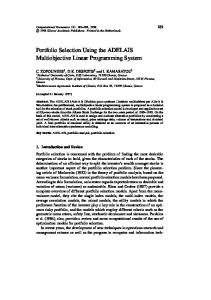
Figure 1: Basic architecture of the system.

Pareto optimal solutions form the so called true Pareto optimal set and its image in the objective space is named the true Pareto optimal front (Coello Coello, van Veldhuizen, & Lamont 2007). Ideally, decision makers must choose a solution from the true Pareto optimal set. If the true Pareto optimal set is not known and exact methods can not be applied, a good approximation may be useful to aid decision makers in selecting the best compromise solution according to their preferences. Traditional optimization methods handle multiobjective problems by means of scalarization techniques. Then, they really work with only one objective obtained by a scalar combination. These methods are not well suited to obtain multiple solutions for a multi-objective problem in a single run. In fact, classical search methods identify one solution at a time, requiring multiple executions to identify a set of different solutions (Coello Coello, van Veldhuizen, & Lamont 2007). Meanwhile, MOEAs have demonstrated to be efficient and effective exploring huge and complex search spaces finding good approximations of the entire true Pareto optimal set for many difficult multi-objective problems in a single run. As discussed in the previous section, when planning the crops to cultivate in a set of land parcels, farm managers have to deal with issues as several crop options and their nutritional requirements, production costs, chemical characteristics of each parcel and the potential economic scenarios. Considering these issues simultaneously the crop selection problem may become difficult to analyze with common tools. Then, this work proposes an optimization framework based on Multi-objective Evolutionary Algorithms to aid decision making in difficult crop selection problems with conflicting objectives, as the one presented in the previous section. Figure 1 shows the general architecture of the proposed model. Main elements of the model are an optimization core, an agricultural science knowledge database, a scenario generator and a solution viewer.

Agricultural science knowledge database contains information regarding soil tests results and optimal application values of fertilizers and aglime. The economic scenario generator module implements the model to generate a database of future feasible scenarios from the historical crop prices and yields of the different considered crops. In this work, information about the mean and variance of the productivity and market values of each crop are used to produce scenarios by generating random variables using normal distribution. Experts using the system may want to analyze some specific scenarios, thus, the system allows the introduction of scenario sets in the database. Both, science knowledge database and scenario database feed the optimization module composed of a MOEA which receives as inputs soil test results and dimensions of each parcel, nutritional requirements of considered crops, a set of feasible scenarios and specific MOEA parameters. The optimization module evaluates candidate solutions searching for optimal ones obtaining a Pareto set of crop cultivation strategies. Finally, solutions are saved in database and passed on to the visualization module. Using the proposed framework, sequential and parallel versions of the Strength Pareto Evolutionary Algorithm (SPEA) (Zitzler & Thiele 1999) and the SPEA2 (Zitzler, Laumanns, & Thiele 2001) were implemented to solve the problem at hand. Detailed information on each implemented MOEA can be found in referenced papers. A general background on various multi-objective evolutionary algorithms is provided in (Coello Coello, van Veldhuizen, & Lamont 2007). However, it is important to point out the most outstanding aspects of these algorithms. First, MOEA works simultaneously with a set of solutions known as evolutionary population. Second, each used algorithm processes its population iteratively using random based genetic operators (as selection, mutation and crossover). It is expected that populations improve from one iteration (generation) to the next one. In this way, a good approximation to the Pareto set may be obtained from the final set of solutions. There are many factors that affects the quality of final solutions obtained by MOEAs as population size, the number of generations and the number of evaluated scenarios. To improve final solutions this work proposes the use of parallel MOEAs (pMOEAs) based on the island model (van Veldhuizen, Zydallis, & Lamont 2003). In island evolutionary algorithms, one population is divided into subpopulations called islands, or regions. The evolution of solutions proceed in each island independent manner. Additionally to the basic operators of evolutionary algorithms, a migration operator which controls the exchange of individuals between islands is introduced. By dividing the population into regions and by specifying migration criteria, the island model adapts well to various parallel architectures. The parallel model used in this work is composed of a collector and several pMOEAs. The collector spawns all pMOEA processes and receives calculated solutions from

Algorithm 1 General SPEA2 algorithm Receive pMOEA input parameters Generates an initial population P randomly, set G = 0 Create an empty archive P¯ Repeat Calculate objective vector F for every solution in P Calculate fitness values of individuals in P and P¯ ¯ Apply environmental selection (update P) if the stop criterion is reached then Send non-dominated solutions in P¯ as finals and exit end if Apply mating selection Use crossover and mutation to obtain a new population P if condition to migrate is reached then Select migrants from P¯ according to a specified criteria Send migrants to all other processes end if if there are received solutions from other demes then Replace individuals in P by received ones end if G = G+1 End repeat

them. In addition, it maintains an archive of the nondominated solutions interchanged between islands and provides the final Pareto approximation set. This process does not utilize any evolutionary operator and does not interfere with the evolutionary process. Meanwhile, pMOEAs perform the real computation. pMOEAs are based on sequential multi-objective evolutionary algorithms that were modified to incorporate a migration operator. Algorithm 1 shows a pMOEA based on the Strength Pareto Evolutionary Algorithm 2 (Zitzler, Laumanns, & Thiele 2001). Initially, parallel SPEA2 receive evolutionary parameters values and a set of feasible scenarios. Then, a randomly gen¯ are erated genetic population (P) and an empty archive (P) created. Once the k optimization objectives are calculated, the SPEA2 fitness assignment procedure is used to rank so¯ Then, the environmental selection prolutions in P and P. cedure proceeds (Zitzler, Laumanns, & Thiele 2001). If the stop criterion is reached, SPEA2 sends to the collector non¯ If the stop criterion is not satisfied, dominated solutions in P. the algorithm continues applying a mating selection procedure which fills the mating pool using binary tournament ¯ After the mating pool is selection with replacement on P. filled, crossover and mutation proceed to produce new offsprings in P. Then, as long as a stop criterion is not reached, the evolutionary process continues. As the number of generations G increases, solutions in P¯ are expected to improve. Then, the final solution set obtained by SPEA2 has the potential to be a good approximation of Ptrue . At each generation, the migration condition is tested. If the migration condition is true, migrants are selected. In this work, the migration condition is based on a probability test. Since there is no unique best solution to migrate, some criterion must be applied. Thus, elements to migrate are considered only among ¯ A paranon-dominated solutions in the current archive (P). meter controlling the maximum number of migrants is pro-

vided. Therefore, migration of individuals is controlled by two parameters, one for the frequency of communications, and another for the number of migrants. Migrating elements may represent a fraction of the non-dominated set of individuals that currently are in a MOEA’s population (Bar´an, von L¨ucken, & Sotelo 2004).

shows that as the average net gains increases also the standard deviation (risk) increases. The bubble size also shows that solutions having great total cost of investment produce the best average net gain.

At the end of the optimization procedure obtained solutions are passed on to the visualization module which presents the solutions to the decision maker who is in charge of selecting one of the proposed solutions to be implemented. Since the delivered solution set may have many solutions these are presented in a grid showing function values. When a row in the grid is selected the crop strategy is shown in the same window. Also, it is possible to click in a button to show the solution in a map as shown in Figure 2.

Figure 3: Snapshot of a bubble graphic with obtained results.

Experimental Results To test the model to be practical, it was run using as optimizers sequential and parallel implementations of the Strength Pareto Evolutionary Algorithm (SPEA) (Zitzler & Thiele 1999) and the SPEA2 (Zitzler, Laumanns, & Thiele 2001) with real data of a cultivable area in Alto Parana, Republic of Paraguay. The employed data is available upon request and it can not be included for paper length constraints. The scenario generator used in these runs is based on normal distribution of historical values. Figure 2: Snapshot of a windows showing a solution.

Besides the proposed objectives there is information that is not used to conduct the search of solutions but is important when a solution is analyzed, particularly, the total, minimum and standard deviation of the net gain corresponding to each solution. These values are not included as objectives while search procedure goes on, since there are directly related to those considered in the multi-objective crop problem defined in the previous section. Because there are relevant factors when the final solution set is presented thus in this point there are included and treated as objectives. There are many solutions and factors that have to be considered. To aid visualization and selection of solutions a window is used to show the solution set considering three objectives simultaneously by means of a bubble graphic. A combo box is used to select which objectives will be shown in each axes and by volume in the graphic. Figure 3 shows a solution set in objective space using the bubble chart window of the visualization module provided by the system. In this case, x axis is for the average net gain, y axis is for the standard deviation of net gain and volume is for the total cost. The graphic

The implemented algorithms provides solution sets having many different cultivation schedules. These obtained result sets were compared in order to determine the best multi-objective approach for system implementation and extensions. Thus, using the same problem parameters, 10 different runs of sequential and parallel versions of SPEA and SPEA2 using 2, 4, and 8 processors were carried out. Results obtained by each implementation were combined and the Pareto Front extracted. As the true Pareto front is unknown, the coverage metric (Zitzler, Deb, & Thiele 2000) was used for a direct comparison of the solution sets. Having two result sets coverage metric indicates the number of points in one set that dominate or are equal to points in the other set. According to comparison results, parallel versions outperform sequential ones and in all cases SPEA2 obtains better solutions than SPEA. In fact, only parallel SPEA with 8 processors obtains solutions that dominates those obtained by the sequential SPEA2. There is not an element in any solution set that is is better or equal than the solutions obtained by the SPEA2 using 8 processors. The full coverage result is also available upon request. Afterwards, results of a parallel SPEA2 with 8 processors run were presented to experts. The graphics tools provided

by the system were used to select alternative solutions in order to analyze them more carefully before selecting one for its implementation. A posteriori analysis of proposed solutions is necessary since the system does not consider the resource allocation problem related to the crop assignment and it does not consider the decision maker preferences during the search for solutions, either. Because the search for solutions does not consider the decision maker preferences a priori, the system is allowed to obtain solutions that may not be considered if a prune of the search space is applied before execution. The system does not consider that, in practice, adjacent parcels are interesting to be of the same kind of crop in order to maximize the use of agricultural machinery and farm equipment. Therefore, an obtained solution may not be applicable without further considerations. These issues must be considered in following extensions of the system to simplify the work that have to be done after the solution set is provided. In spite of this, it is very useful for the decision makers to see the many alternative solutions proposed by the system in order to gain insights in the problem domain before making a final selection as shown in Figures 2 and 3.

Conclusions This work proposes for the first time a model based on Multi-objective Evolutionary Algorithms to solve a multiobjective crop selection problem considering five different objectives and crops simultaneously. Using the proposed model, both sequential and parallel implementations of two MOEAs were implemented as optimizers. A comparison between the different implementation was carried out using the coverage metric. For the implemented test problem, the pSPEA2 with 8 processors appears to be the best suited optimizer for the problem at hand. The obtained solutions were passed on to a visualization module that graphically may show solutions to decision makers for them to select one of these for further analysis and implementation. The visualization module shows the various obtained solutions and objectives helping decision makers to gain insight about the problem at hand. This way, according to the expert’s preference, the implemented tool may be used to aid the selection of a solution that will improve soil usage, reduce cultivation costs, minimize economical risks, maximize the economical return, adjust fertilization use to a given budget and minimize the environmental impact of cultivation process. Future works include the use of the proposed framework using other multi-objective metaheuristics as optimizers. It is also proposed to extend the solution model to include the related resource allocation issues. A planning scope of various years may also be considered. Another future work is to include the decision maker’s preferences in an interactive way while the search procedure goes on. It is important as well to improve the tools to show multi-objective solutions.

References Baker, R.; Ball, S. T.; and Flynn, R. 2002. Soil analysis: A key to soil nutrient management. Technical report, Cooperative Extension Service College of Agriculture and Home Economics. New Mexico State University. Bar´an, B.; von L¨ucken, C.; and Sotelo, A. 2004. Pump scheduling optimization using asynchronous parallel Evolutionary Algorithms. CLEI Electronic Journal 7(7). Bocco, M.; Sayago, S.; and Tartara, E. 2002. Multicriteria models: an application for the selection of productive alternatives. Agric. Tec. 62(3):450–462. Chi-Mei, L.; Lan, L.; Zhi-Qiang, Y.; and Ding-Xin, P. 2002. Sustainable use of land resource and its evaluation in county area. Chinese Geographical Science 12(1):61–67. Coello Coello, C.; van Veldhuizen, D.; and Lamont, G. 2007. Evolutionary Algorithms for Solving Multi-Objective Problems. Springer, second edition. Johnson, S. L.; Adams, R. M.; and Perry, G. M. 1991. The on-farm costs of reducing groundwater pollution. American Journal of Agricultural Economics 73(4):1063–1073. Kelling, K.; Bundy, L.; Combs, S.; and Peters, J. 1996. Soil test recommendations for field, vegetable and fruit crops. Extension Publication A2809. Matthews, K.; Craw, S.; Elder, S.; Sibbald, A.; and MacKenzie, I. 2000. Applying genetic algorithms to multiobjective land use planning. In Whitley, L.; Goldberg, D.; Cant´u-Paz, E.; Spector, L.; Parmee, I.; and Beyer, H., eds., GECCO. Morgan Kaufmann. Schroth, G., and Sinclair, F., eds. 2003. Trees, crops and soil fertility: concepts and research methods. CABI Pub. Stewart, T. J.; Janssen, R.; and van Herwijnen, M. 2004. A genetic algorithm approach to multiobjective land use planning. Comput. Oper. Res. 31(14):2293–2313. Tsuruta, J.; Hoshi, T.; and Sugai, Y. 2001. Selecao de areas adaptativas ao desenvolvimento agr´ıcola, usando-se algoritmos geneticos. Technical report, EMBRAPA, Brazil. van Veldhuizen, D.; Zydallis, J.; and Lamont, G. 2003. Considerations in Engineering Parallel Multiobjective Evolutionary Algorithms. IEEE Transactions on Evolutionary Computation 7(2):144–173. Yu, L.-Y.; Ji, X.-D.; and Wang, S.-Y. 2003. Stochastic programming models in financial optimization: A survey. AMO — Advanced Modeling and Optimization 5(1). Zitzler, E., and Thiele, L. 1999. Multiobjective Evolutionary Algorithms: A Comparative Case Study and the Strength Pareto Approach. IEEE Trans. on Evolutionary Computation 3(4):257–271. Zitzler, E.; Deb, K.; and Thiele, L. 2000. Comparison of Multiobjective Evolutionary Algorithms: Empirical Results. Evolutionary Computation 8(2):173–195. Zitzler, E.; Laumanns, M.; and Thiele, L. 2001. SPEA2: Improving the Strength Pareto Evolutionary Algorithm. In EUROGEN 2001. Evolutionary Methods for Design, Optimization and Control with Applications to Industrial Problems.